Exploration of Applications with Concentrating
Solar Arrays
David Kelly
Physics, BA; Mathematics, BA
University of North Carolina at Chapel Hill
[email protected]
April 14,2014
Abstract
Nomenclature
Symbol Name Value Unit
α Seebeck Coefficient µV/K
δ Earth Declination Angle deg
˙
Qh Hotside heat Flow Rate W
˙
Qh Rate of heat flow W
η Efficiency %
γ Concentrator Facing Direction deg
ω Solar Hour angle deghour
Ω Solid angle Sr
φ Latitude
π Peltier Coefficient W/A
ρ Electrical Resistivity Ωm
σ Stefan-Boltzmann Constan 5.60373×10⁻⁸ W m−2K−4
τ Thomson Coefficient
θ Angle between Aperture normal and Sun
direction
deg
ε Emissivity
Aa Collector Aperture Area m2
C Specific Heat J/K
D Distance to heat source mm
E Seebeck EMF V
GSC solar constant 1367 W/m2
h Convective heat transfer coefficient W/m2K
H0 Horizontal Surface Radiation, no atmo-sphere
W/m2
Hb Direct Beam radiation W/m2
Hd Diffuse sky radiation W/m2
Hg Horizontal surface Radiation W/m2
k Thermal conductivity W/mK
KT Clearness index
L Plane wall thickness m
M Mass kg
Nd day number 0<1<365
Nu Nusselt Number
q Rate of heat flow W
rd ground diffuse Reflectance
Ra Rayleigh Number
Tamb Ambient Temperature K
Tc Cold Side temperature K
tclock Respective time of observer
ts Solar time
A Cross Sectional area m2
a Effective Width of TEG mm
b Effective Length ot TEG mm
d Parabolic Diameter m
f parabolic Focal length m
h Parabolic height m
I Current A
I Irradiance W/m2
l Length of Parabolic Trough m
n,m,N Number
P Power W
R Resistance,Electrical Ω
T Temperature K
1
Introduction
In 1823, following the heyday of the industrial revolution, steam engines were the work horse machines of the time. With environmental and sustainability concerns almost cer-tainly being non-existent, these machines operated at roughly 3% efficiency. Though this is not an astounding efficiency, and it certainly would not do by today’s standards, these machines enabled and facilitated the industrial revolution. At this same time, however, Thomas Seebeck made an important discovery that could be the path to clean and efficient energy today. Seebeck observed that an electrical potential was built up when a junction of two different conductors was exposed to a temperature gradient. That is, he discovered an important property which can be used to convert thermal energy directly into electricity. Had he been able to combine some of the materials he was researching, he could have easily created a heat engine which was every bit as efficient as the steam engines of his time [15].
This alternative heat engine would not come into being for many years, though, due to Michael Faradays discovery of the connection between electromotive force and mag-netic flux. Though Thomson and Peltier would later go on to make important discoveries relating to thermoelectric properties, these effects would remain relatively unstudied for decades. This lack of interest has left the thermoelectric generators of today at a relatively low efficiency in comparison to other electricity generators. However, unlike in Seebecks day, our power production methods today necessitate a high degree of environmental con-cern. As the need for clean and reliable energy resources increases, alternative production methods must be explored. Currently thermoelectric generators, while they are not incred-ibly efficient, have a promising future in various applications. The aim of this research, like many other current studies, is to explore a facet of those applications and assess the possibility of using these devices to capture and use naturally available energy.
1.1
Current Research
The thermoelectric effects (which will be described in the following sections) are the sub-ject of a broad range of research topics. From system applications to materials research to the atomic-level physical interactions, the thermoelectric explorations are quite diverse. While the material research is an interesting topic, and certainly plays a role in the poten-tial power production of TEGs, this study aims to examine the application aspects of these devices and is thus not entirely concerned with the current topics of materials research as they relate to the thermoelectric phenomena. A brief description of material properties will, however, be included in following sections.
1.1.1 Direct Power Generation
One obvious use of thermoelectric devices is direct power production. To be specific, there are many applications in which thermoelectric devices could be used solely to pro-duce electricity. As a matter of fact, the physical experiment that is the subject of this report is a direct power generation application. These direct power generation applica-tions can be grouped as follows.
Synthetic Heat Sources
A simple application of TEG systems is to create some heat-releasing reaction, and use the TEGs to capture some of expelled energy. These include various thermo-chemical re-actions (such as combustion or nuclear decay), which act as a energy resource for the TEG to produce electricity from. In fact, these synthetic heat sources are utilized in conjunction with thermoelectric devices largely in space applications. The mars rover Curiosity has an on board radioisotope thermoelectric generator to power its mission [10]. While space applications are very viable applications of thermoelectric technology with synthetic heat sources, the low efficiency of TEGs prevents them from being widely used with, say, com-bustion reactions because there are much more efficient means of capturing energy from these reactions currently.
Natural Heat Sources
As an alternative to synthetic heat sources, many scientists are exploring the use of TEGs in conjunction with natural heat sources. These sources can have a broad range in nature. From concentrated solar, solar ponds and even geothermal sources, there are many natural sources of energy which could provide renewable sources from which TEGs could draw their power [22, 17]. The aim of this report is to explore an application of this type.
Waste Heat Sources
A final category of direct power production, and possibly the most favorable application of current TEG technology, is the conversion of waste heat into electricity. Many, many processes produce waste heat. The combustion engine for example wastes 70% of the combustion energy in heat. Nearly all large scale power production is by means of thermal reactions. Thus, there is an inherent loss of energy. Many are researching how to effec-tively utilize TEG systems to capture this waste heat. Whether in capturing the energy lost to friction, or in increasing the overall efficiency of other power producing methods [8].
1.1.2 Cogeneration
offer an increased overall efficiency in use of captured energy, and present multifaceted approaches to solving energy needs.
Primary TEG Power, Secondary Heat
Here, energy is directed to a TEG array, and electricity is first produced. Then, the heat that is rejected from the TEGs is utilized as a source of heat. For example, one application being explored is using a concentrating solar system to collect heat for TEGs, then the rejected heat is used to heat residential water [16].
Primary Heat, Secondary TEG Power
In this case, energy captured first to act as a heat source, and then a TEG system is used to siphon off a fraction of that energy to produce electricity. For example, energy may be used to heat water, and then a TEG system is used to capture some of the thermal energy and convert it to electricity. This could see large use in situations in which water is heated beyond a common usable temperature. Here, TEGs could, by removing some of the ther-mal energy of the water, not only reduce the temperature of the water, but also produce electricity at the same time [14].
1.2
Purpose of Study and Hypothesis
Water Holding Tank
Cooling pipe TEGs attached to underside
along focal line
Parabolic mirror
Water flow direction
Figure 1: A square pipe with TEGs attached to the underside is oriented along the focal line of linear parabolic mirror. Water is pumped through the pipe to disburse the waste heat energy from the TEGs.
directly in an effort to reduce energy losses. Furthermore, a cooling system is necessarily required for thermoelectric power production. Given its availability and high specific heat, running water is used to dissipate the waste heat energy from the system. Thus, in theory focusing solar energy directly onto the face of thermoelectric devices, and by cooling them with a running water system, provides a system which is suitable for large scale power production.
To test this hypothesis, a system as in Figure 1 is used. A linear parabolic mirror is used to concentrate solar energy onto the face of three TEGs. Moreover, these devices are connected to what will be called the ‘cooling assembly’. A square aluminum pipe provides a flat surface to which the TEGs are connected. Water is moved through this pipe to help dissipate the unused solar energy from the TEGs. A theoretical analysis will describe and quantify the potential electric output in this type of situation, and a physical experiment will be used to verify and further test these theoretical findings. These endeavors are specifically aimed to determine if a system such as this can be scaled to be used either in commercial power production, or to be used in a private residential situation. To begin, a brief description of current thermoelectric research is given.
2
Thermoelectric Properties and Theory
To begin to rigorously study and analyze the potential of the proposed system, it is im-portant to understand the thermoelectric phenomena. It will be essential to first develop an understanding of the physical effects which enable thermoelectric power generation. Following this, a brief look into the thermal nature of these devices and the use of semi-conductor materials will lead into a discussion of the power generation capabilities of thermoelectric devices. These developments will provide a strong physical basis from which the capabilities of the proposed system are built upon. To begin, the thermoelectric phenomena are described.
2.1
Thermoelectric Effects
There are three key effects which are generally presented on the subject: The Seebeck effect, the Peltier effect, and the Thomson Effect (each named for the scientist who first discovered them). Making use of the simple model in Figure 2, these effects are briefly defined here following Pollock’s, Dechers and Joffes descriptions [13, 7, 5].
2.1.1 Seebeck Effect
T T+ΔT Conductor A
Conductor B
(a)
T T+ΔT
Conductor A
Conductor B
dqAB dqBA
(b)
T T+ΔT
Conductor A
Conductor B
dQB
dQA
(c)
Figure 2: Thermodynamic circuit to explain Seebeck, Peltier and Thomson effects. Pollock’s work [13].
and the other is heated, then the particles in the hot end of the box will gain more kinetic energy than those at the cool end. As such, these particles will begin to move around the box. Since the cool particles are relatively stagnant, the hot particles will tend to move to the cool end much more quickly than the cold particles move into the hot end of the box. Now suppose these particles are charge carriers. As the hot charge carriers move towards the cool end of the box, there will be a build up of charge at that end, resulting in an overall electrical potential across the box. This is as Teutsch states “a tendency for heat to drag along electricity” [19]. Furthermore, theabsolute Seebeck coefficient, α, denotes the rate
of change of this potential as it depends on temperature for a specific material. While an absolute Seebeck coefficient proves difficult to determine, a relative Seebeck coefficient is more easily found.
Consider Figure 2a. The absolute Seebeck effect dictates that an electrical potential will be generated in each of conductors A and B. Then, the relative difference between these two potentials produces an electromotive force (EMF)EABin the wire. This is called therelative Seebeck EMF. The rate of change in this EMF at a given temperature is the
relative Seebeck coefficient, given by
αAB=
dEAB dT
T
Thus it is clear that α is given in units ofV/K. Specifically, the Seebeck coefficient for
many thermoelectric generators are on the order of 200−300 µV/K. As will be shown
in the following section, the thermodynamic nature of this relative EMF allows for the thermoelectric characterization of many materials.
2.1.2 Peltier Effect
Due to the resultant current that is produced by the relative Seebeck EMF, thePeltier Effect
is the absorption or expulsion (reversible) of heat at the junction between two conductors. This is shown in Figure 2b with an external power source. As current flows across the boundary between two conductors, heat will either be given off or taken in at that junction. ThePeltier coefficientπAB, then, is the change in heat content Qat the junction between
A and B as it relates to the currentI,
πAB=
This absorption and rejection of heat has found widespread use in cooling technologies. Peltier plates, as they are commonly called, can be found in diverse applications from water tanks to computers. Moreover, the reversible nature of Peltier effect gives rise to the heat engine qualities of thermoelectric generators.
2.1.3 Thomson Effect
Similar to the Peltier Effect, theThomson Effect dictates that heat is evolved or absorbed as current passes through a single conductor in a temperature gradient, shown in Figure 2c. As current passes through a homogeneous wire whose ends are held at different tem-peratures, heat is given off or absorbed throughout the length of the wire. Therefore, the
Thomson coefficientτrelates the heatdqgiven off (or taken in) by a wire to the currentdI
flowing through it and its imposed temperature gradient∂T/∂xover a lengthdxas
dq=τdI∂T
∂xdx
Here it is important to note that this is very different from Joule heating. The Thomson effect is independent of the resistive qualities of the material, while Joule heating is related to the resistance of the conductor (it is often called ‘resistive’ heating). Furthermore, the Thomson effect is due to a temperature gradient imposed on the conductor to which Joule heating nominally has no relation. Moving forward, the thermal nature of the Thomson effect and the other thermoelectric effects are used to relate these three effects.
2.2
Thermodynamic Considerations
Continuing to use Figure 2, we can now consider the thermodynamic relationship between each of these three effects. Denoting the relative Seebeck EMF generated in this closed loop due to the temperature difference asEAB the relative Seebeck coefficient isdEAB/dT,
and thus the electrical power is
IEAB=I
dEAB dT ∆T
and thus, eliminating the common current term on each side
EAB=dEAB
dT ∆T
Furthermore, the Peltier and Thomson Effects contribute to the net thermal energy of the system. The Peltier effect will contribute to energy absorbed and released at the junctions, while the Thomson effect will lead to a similar energy exchange in each of the conductors themselves. The balance of energy in this circuit mandates that the electrical power pro-duced from this temperature gradient must be matched by the rejection and absorption of heat both at the junctions and across the two conductors [5], thus
dEAB
Then, continuing to follow Pollock’s derivation [13], dividing through by∆T gives
dEAB dT =
πAB(T+∆T)−πAB(T)
∆T + (τB−τA)
Letting∆T approach zero, it is seen that
dEAB dT ∆T =
dπAB
dT +τB−τA
Thus we have shown a fundamental linkage between the electrical potential (Seebeck ef-fect) and the thermal potentials (Peltier and Thomson effects) of the thermoelectric phe-nomena. A distinct relationship between thermal characteristics (temperature) and electri-cal potential (EAB) has been shown for a thermocouple as in Figure 2. This relationship is
critical for the production of power from thermoelectric materials. Furthermore, relation-ships between each ofα,τandπcan be shown through various entropy and conservation
considerations [7]. With these relationships it is possible to describe the thermoelectric power production entirely in terms of the Seebeck coefficientα. Additionally, it is
impor-tant to note that the relative Seebeck coefficient is independent of a flowing current. Thus, considering an open circuit, the relative Seebeck coefficientdEAB/dT is given by
dEAB
dT =αA−αB
whereαAandαBare the absolute Seebeck coefficients of conductors A and B respectively.
This fact presents a key quality which is utilized, in conjunction with the other thermody-namic relationships, to evaluate the thermoelectric effects in different materials. That is, given this equation, it is possible to build up a knowledge base of Seebeck coefficients for various materials.
The absolute Seebeck coefficientα then is directly related to electrical potentialEAB
by means of a temperature gradientdT. Thus, for any two conductors there are a number of relationships that may exist betweenα for each material. Specifically, there are two
extreme cases: either each ofαA and αB increase at the same rate with temperature, or
they diverge at exactly opposite rates with temperature. Generally, the latter case is unfa-vorable due to its non-linear nature. The former case is most desirable, and has lead to the widespread use of semiconductor technology in thermoelectric devices.
2.3
Power Generation
Simple inspection of the respective units of the Seebeck coefficientα (V/K) and the
tem-perature gradient ∆T (K) lead one to see that the voltage across a load resistance as in
Figure 3a is
V =α∆T
Furthermore, because the p and n legs of a thermocouple are in series, the internal re-sistance of a single thermocouple is given by the sum of the rere-sistance of each of these legs
RL
p n
Th
Tc
(a)
n couples in Series
m couples in Parallel
RL
(b)
Figure 3: (a) shows a single thermocouple made of p-type and n-type semiconductor materials in dark and light blue respectively. The two ends of the couple are held at Th and Tc. (b) Diagram
of thermoelectric generator with load resistance RL. Here the blue squares represent each of the
n×m total thermocouples.
Additionally, each p and n leg has its own electrical resistivityρi. Thus, for legs of length
Land cross sectional areaAi, the total internal resistanceRof a single thermocouple is
R=
ρp
Ap L
+
ρn
An
L
Therefore, the current across the load resistanceRL is
I= α∆T
R+RL (1)
Given a known temperature gradient (∆T) and material parameters (α,R) it is straight
forward to find the power output from a single couple. That is, using Ohm’s law, the power outputPin watts will be given by
P=I2RL=
α∆T
R+RL
2
RL
However, power producing thermoelectric devices rarely will use a single couple. Ref-erencing Figure 3b, first considern thermocouples in series. The current across the load resistance is
I= nα∆T
Rtot+RL
typical to connect thermocouples in parallel to boost overall performance. Then, if there aremof thesenRchains in parallel, then the internal resistance is given as
Rtot =
1
1/nR+1/nR+· · ·+1/nR=
1
m/nR = nR
m
The power output for a general thermoelectric device is
P=I2RL=
nmα∆T
nR m +RL
!2
RL (2)
Equation 2 will be especially useful in modeling and predicting the performance of the TEGs within the proposed system. Typically, the total internal resistance and the total number of couples in a device are listed. For a working version of Equation 2 we can let
Nbe the total number of couples, andRbe the total internal resistance, giving
P=
Nα∆T
R+RL
2
RL (3)
The∆T term in this equation will lend this analysis easily to determining device
perfor-mance and efficiency.
2.4
Efficiency
As with any system doing work, the efficiency of a TEG will be given by the ratio of useful work done to the input energy. In the case of this electrical system it is pertinent to look at the electrical power. Generally, the efficiencyη is
η=
P
˙
Qh
where ˙Qh , in units of watts, is the flow rate of heat onto the hot side of the device. By considering the reversible energy flowing through an element due to the Seebeck, Peltier and Thomson effects, as well as the irreversible energy flow due to resistive heating, Joffe [7] shows that
˙
Qh=α(Th−Tc)I+K(Th−Tc)−
1 2I
2R
whereK is the total thermal conductivity of the device. The efficiency, then, using P=
I2RL, is given by
η= I
2R
L
α(Th−Tc)I+K(Th−Tc)−12I2R
η=
Th−Tc Th
×
m m+1
1+KR α2 ×
m+1
Th − 1
2(Th−Tc)
1
m+1
(4)
First, Equation 4 shows that the temperature difference Th−Tc across the device is
critical for the overall efficiency. Being able to maintain this temperature gradient will facilitate higher efficiencies. Furthermore, the term KR
α2 captures all of the material
prop-erties of the device. The figure of meritZ is the inverse of this term and gives a measure of the electrical properties as they relate to the thermal properties in a material. For a thermocouple this is defined as
Z= (αp−αn) 2
KR
whereαp andαn are the respective Seebeck coefficients for the p- and n-type elements.
Using this term, the efficiency can be optimized for the ratiom. To find maximum effi-ciency as it relates to this ratio, we simply look for roots of the derivative of the effieffi-ciency as it relates to m
∂ η
∂m=0
Solving shows the optimal ratio of the internal to the external resistance (RL/R)opt,
de-noted asM, is
RL R
opt
=M=
r
1+1
2Z(Th−Tc)
Then using this in Equation 4 we find
η=
Th−Tc Th
× M−1
M+Tc
Th
It is clear that ifM>1 then efficiency suffers. So there are two consequences. First, the load resistance needs to match the internal resistance. This is often called ‘load matching’, and will be a key topic in analyzing the performance of the proposed system. Second,M
depends onZ. The desire is to match Z with a given application. Furthermore, Z shows that it is desirable to have materials with low thermal conductivity and a low internal resistance (or in other words, high electrical conductivity). While many metals have high electrical conductivities, they are also fairly good thermal conductors. Hence, thermoelectric devices often make use of semiconductor materials. The theory of these materials as they relate to thermoelectric devices is developed in the following section.
2.5
Thermoelectric Transport Theory
out of a material with a high electrical conductivity, and a low thermal conductivity. Ther-mal energy is carried through a material by either freely moving particles (electrons) or by waves passing through the lattice structure (phonon).
In a metal, the sea of electrons freely moves current with ease. However, these elec-trons also are the primary carriers of heat through the material. Thus the electrical and ther-mal conductivity of metals are intrinsically coupled to the movement of electrons through the material. Hence metals are not the usual choice of material for thermocouples because of the relative inability to increase electrical conductivity without also increasing thermal conductivity.
Semiconductors, on the other hand, have a slightly decoupled modes of heat and elec-tricity transport through their material. Here, because the electrons do not readily form the same ’sea’, phonons play a more significant role in the transfer of heat through the ma-terial. Thus, in essence, semiconductor materials are able to facilitate heat and electrical conduction via two different pathways. Because these pathways are now separate, if only slightly so, materials can be engineered so that thermal conductivity decreases while elec-trical conductivity increases. Therefore semiconductor materials are the ideal in creating thermocouples.
3
Solar Resource and Concentrating Methods
The sun’s radiation will be the source of energy within this study. Accordingly, it is neces-sary to characterize this resource. To begin, the sun is commonly treated as a black body radiator. As such, it emits its energy (in the form of electromagnetic waves, or more sim-ply, light) in all directions radially from its surface. Of particular interest is the light which is headed towards the earth. As this light travels across the cosmos it sees little impedance until it reaches the earth’s atmosphere. Here the light is absorbed, reflected, or unhindered. The NREL has compiled solar radiation data for various locations throughout the US over a 10 year span [11]. Taking Raleigh as a good approximation for Chapel Hill, concen-trating solar devices see a daily average of 4.4 kWh/m2/solar radiation which is parallel to their parabolic axis. Given roughly 10 hours of sunlight in a day, this means that there is, at any given moment during the day, 4400 W/m2 of usable solar radiation. This is a vast amount of power and capturing as much of that energy will be of primary concern.
Making use of this radiant energy is an interesting problem for which there are many solutions. One method is to concentrate the energy to a small location and use the resultant temperatures to do thermodynamic work. In order to maximize the total energy that can be used with such a method it will be important to not only understand the underlying concepts of concentrating collectors, but to also understand the movement of the sun.
3.1
Concentrating Collectors
to a small point or line, concentrating collectors are able to attain much higher tempera-tures, and do so with little to no input energy. There are several advantages associated with concentrating methods. First, because the sun’s energy is focused to a small point, these collectors are able to attain relatively high temperatures. In fact, the Solana power plant project will be able to generate temperatures upwards of 380◦C [12]. Second, the small area to which the radiation is focused helps to reduce convective losses. Furthermore, because reflective surfaces are generally far less expensive than absorbing surfaces [18], concentrators provide an economic advantage to non-concentrated methods. Therefore the renewable nature of this research is centered about the use of concentrated solar en-ergy. What follows is a brief description of the concentrating geometry which will be used in this application, followed by a discussion on some of the limitations of concentrating methods.
d
h
f
x y
Focal Point
(a)
Focal Line
Aperture Mirror Surface
(b)
Figure 4: (a)Parabola and its dimensional variables, (b) Linearly translated parabola with its aperture and focal line pointed out
3.1.1 Solar Trough Geometry
A parabola is a fairly simple geometrical shape that acts as the backbone of concentration optics. The useful quality of the parabolic geometry is in its ability to re-direct light to a single point. That is, any beam of light which is parallel to the parabolic axis (the x-axis in the case of Figure 4a) is reflected to the focus point. To locate the focus point in terms of easily measured dimensions, an equation for a general parabola opening to the x-direction is
where f distance from the origin to the focal point. Using Figure 4a, then to relate the height of the parabolahto the focal length, we may set y=d/2 andx=h in Equation 5 to find
h= d 2
16f
or, rearranging
f = d 2
16h (6)
Therefore, Equation 6 gives the focus point of a parabola in terms of its heighthand its aperture diameterd. These are easily measured for any parabola and thus provide a rather accessible calculation of the focus point.
If a parabola is translated along a line, the surface it forms is called a parabolic cylin-der. More commonly this shape, shown in figure 4b, is referred to as a parabolic trough. Furthermore, this translation turns the focal point into a focal line. All light parallel to the parabolic axis that falls within the aperture of the trough will be directed to the focal line. For a trough of lengthl and parabolic diameterd, the area of the apertureAais given by
Aa=ld
Unlike a parabolic dish (where a parabola is rotated about its axis), which has only a focal point, the focal line of a solar trough is very adaptable to different systems. One such example is solar water heating. Here, a pipe is able to be positioned across the focal line, and water pumped through it. In a similar way a parabolic trough is used in this study to focus light onto a row of TEG devices, which are cooled by a pipe running across the parabolic trough. The linearity of the trough is ideal for flowing water systems.
3.1.2 Limitations of Concentrating Methods
Because a trough shape is open on its ends, it is possible that light will be reflected beyond the edge of the device. To be specific, if the source of light is on the left most side of the trough, then light which hits the right most side will be reflected even further to the right. This is often termed ‘end loss’. While it may not be a significant reduction in overall collected energy, it is a problem that is not present in parabolic dishes.
As mentioned in the previous section, a parabola is able to focus light which is parallel to its axis. While this is the alluring quality of a parabolic trough, it is also a very cir-cumstantial. More specifically, the parabola is only able to focus light which isparallelto its axis. A parabolic mirror will not be able to make any significant use of light from any other direction. Therefore it is critical that the device point directly to the sun. The facing direction and tilt of the device will be critical in capitalizing on light rays that are parallel to the parabolic axis.
3.2
Device Tilt and Facing Direction
N φ S Sun
Aperture area
β
Facing
Direction γ
North
East
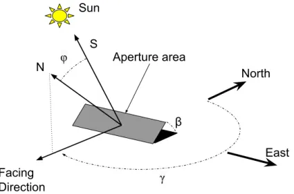
Figure 5: Various angles involved in determining proper tilt and facing direction for a solar col-lector.
irradiance that the aperture seesIaperturethen will be given by
Iaperture=Isuncosϕ
where ϕ is the angle between the normal vector of the aperture N and the unit vector
pointing directly from the aperture to the sunS[18]. Referring to Figure 5, these angles may be seen more clearly. Therefore, it is desirable to adjust the array such thatϕ =0.
Pointing the device directly towards the sun is a simple concept, however it is the subject of rigorous astrophysics. To be brief, the daily spin of the earth, its rotation around the sun, and its seasonal declination angle δ, give a time varying (hourly, daily, seasonally)
path of the sun which the device must track. Therefore, the optimum angle of tilt of the deviceβ (measured from horizontal), and the ideal cardinal facing directionγ (measured
from true North) will be dependent on position of the sun and the declination of the earth at a given moment. First, these parameters will be described briefly, then using an algo-rithm presented by Calabro [3] the optimum angle and direction can be determined for the device.
3.2.1 Solar Position
The earth’s rotation is often described in terms of its hour angleω. In effect the hour angle
describes an observer’s location in reference to the time when the sun reaches its highest point in the day. Technically,ω is the angle between the meridian of the observer, and the
meridian which is directly in line with the sun. A meridian line is one which is drawn on the surface of the earth’s sphere from the north pole through the equator and down to the south pole (i.e. longitude lines). The hour angle is defined in terms of the solar timetsby
It is important to note that the solar time is not quite the same as the standard clock time. Specifically, solar time is a 24 hour system in which 12:00 corresponds to the time when the sun is directly south of an observer (for an observer in the northern hemisphere). Thus the solar time will vary based on the day of the year Nd (out of 365 days). A general equation for the solar time is given by
ts=tclock+ (0.258 cosx−7.416 sinx−3.648 cos 2x−9.228 sin 2x
where
x= 360(Nd−1)
365.242
3.2.2 Earth’s Declination Angle
While students learn early on in their education that the earth revolves around the sun, it often goes unmentioned that the earth ‘wobbles’ along this path. During spring the northern hemisphere leans towards the sun, while in the winter the the earth is leaning away from the sun. This lean will certainly have an effect on the observed path of the sun across the sky. The declination angle of the earth δ is defined as the angle between the
equatorial plane and the line drawn from the center of the earth to the sun. An approximate equation to giveδ in terms of the day numberNd is
sinδ =0.339795 cos(0.98563(Nd−173)) (7)
3.2.3 Cardinal Facing Direction
A final parameter of importance is the cardinal direction which the array faces. Measuring from North, with clockwise angels being positive,γ will be used to describe the facing
di-rection of the aperture. To be specific,γ is the angle between true North and the projection
of the normal line of the aperture onto the horizontal plane. It is rather difficult to de-fine the facing direction when the aperture is perfectly horizontal. However, as discussed earlier, it is not typical or ideal to hold a collecting surface at a zero tilt.
Typically for the Northern Hemisphere a solar collection array is pointed due South,
γ=180◦. Noting that this is obviously not ideal as the sun moves across the sky during the
3.2.4 Determining Ideal Angles
Finding the ideal angle to tilt a solar collector is a rather complicated issue, as has been prefaced in the previous sections. However, there are simplified and fairly straight forward approaches to determining the proper angle. One such algorithm is outlined here based on Calabro’s work [3]. First, there are a few terms which need to be defined. The daily radiation on a horizontal surface without the effects of an atmosphere isH0. This can be approximated by
H0=86400GSC
π ×
1+0.033 cos
2π Nd
356
cosφcosδ
×
±
q
1−tan2φtan2δ
+cos−1(−tanφtanδ)×sinφsinδ (8)
whereGSC =1367 Watts/m2 is the solar constant, Nd is the day number, δ is the solar
declination andφ is the latitude of the device.
Furthermore, a clearness indexKT can relate this radiation to the daily radiation on a horizontal surfaceHg(in the presence of an atmosphere), by
KT =
Hg H0
Note that Hg is an observed radiation and is easily found in published data tables [11].
This global horizontal radiation is made up of a horizontal diffuse sky irradiationHd and a direct beam irradiationHb. The clearness index is also related toHdby
Hd Hg
=1.35−1.61KT
Then, usingH0,Hd,Hg, and the diffuse reflectance of the groundρd, the ideal tilt angle
from horizontalβ, and cardinal directionγ can be determined for a specific sun angleω.
β =tan−1
(
H0×(cosδsinφcosωcosγ−sinδcosφcosγ+cosδsinγ ω)
×
H0+Hd
2 −
Hgρd
2
×(sinδsinφ+cosδcosφcosω
−1)
(9)
γ =tan−1
cosδsinω
cosδsinφcosω−sinδcosφ
(10)
Therefore, in a straight forward fashion one can calculate find the ideal tilt angle and cardinal direction given these formulas developed here. Given radiation data (Hg,rd), and
P
Q̇C
Q̇H Q̇AL1-W Q̇W-AL2
Q̇AL2-Amb
Q̇W-Amb
TEG Parabolic
Mirror
Cooling Assembly Front wall
of Pipe
Back wall of Pipe Cooling Water
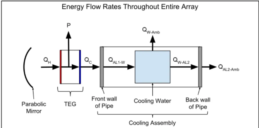
Energy Flow Rates Throughout Entire Array
Figure 6: Energy Flow Rates through out entire array. Theses rates are related to the thermal properties of the materials and will be described in the following sections
4
Thermal Considerations
The thermal properties of this system will be the critical factors in determining the overall power output of the array. Therefore, it is important to consider the ways in which heat energy moves through the system. Specifically, we wish to see how energy will enter the system, how it will leave the system, and the net gain of energy for each piece in the system (here ‘piece’ will refer either to the cooling pipe, water in the pipe, or the water in the holding tank). The power production of the TEG is dependent on the hot and cold side temperatures, thus this analysis is primarily concerned with understanding the factors that affect these temperatures. Many of the thermal properties involved in such a system are described here, and some will be used in later sections to analyze and predict the performance of the system.
4.1
Energy Entering System
Solar Energy will be radiated onto the face of the devices through the mirror surface (or in the case of controlled experiments, directly from the heat source). Here we develop an understanding of quantifying radiation energy. Radiation sources will be treated at black body radiators. The Stefan-Boltzman law states that the total energy radiated per unit surface area j∗ of a black body is directly proportional to the fourth power of the its temperatureT
j∗=σT4
Whereσ=5.670373×10⁻⁸W/m2K4is the Stefan-Boltzmann constant. This same
prin-cipal may be used in the case of reflection. However, if a body absorbs part of its incident radiation, then the power radiated from its surface will be
whereε is the object’s emissivity and is less than one. Then in terms of the total powerP
radiated form the object the equation becomes
P=A j∗=Aε σT4
Where A is the unit area area which receives the radiation. Rearranging, then will give the power inW/m2,P/A, as
P
A=ε σT
4 (11)
The conservation of energy mandates that the power radiated from a sourcePwill be equal to the difference between the power radiant on the hot side of the TEGsPhand the power radiated to the ambientPamb.
P=Ph−Pamb
Applying Equation 11 gives
P
A=ε σ T
4
h −Tamb4
(12)
where Th and Tamb are the hot side temperature and ambient temperatures respectively. Thus we have developed an equation to describe the heatPradiated from a body.
4.2
Transfer of Energy Within the System
Figure 6 shows a broad overview of the energy transfers within the system at any given instant. The main focus will be on the transfer of energy from the cold side of the TEG to and through the cooling assembly. Since these pieces are in direct contact, the energy will move via conduction. In general the rate of heat diffusing across a plane wall is
q= T1−T2
Θ (13)
whereT1and T2 are the temperatures on the face of either side of the wall. The thermal resistanceΘis given by
Θ= L
KA
withL being the thickness of the wall,A being the cross sectional area perpendicular to the direction of heat flow, and K being the thermal conductivity of the wall material in
watts/mK. Specifically, this equation will be used to find the energy conducted from or to the aluminum piping.
Lastly, each piece of the cooling assembly will gain energy. This will inherently lead to an increase in temperature. The change in temperature of each piece can be related to the instantaneous energy it gainsdQby
dQ=MC(Tf−Ti) (14)
whereM is the mass of the piece,C is its specific heat, and Tf and Ti are the finial and
4.3
Dissipation of Energy Away from the System
Continuing to refer to 6, it is clear that energy will exit the system via convection. For a body at a given temperature the rate of heat convection is
q=h(T−Tamb) (15)
whereT is the temperature of the piece andTamb is the ambient air temperature. The con-vective heat transfer coefficient h is a rather complicated function of the cross sectional area, the width, and any surrounding conditions about the piece. A more simplistic ap-proach will be necessary in this situation. Here it is useful to first consider the Nusselt numberNu. This dimensionless term gives the ratio of the convective heat transfer to the conductive heat transfer at the boundary of a material
Nu=hL
K
Thus ifNuis near 1, the conduction and convection processes are near equal in magnitude. For large values of Nu the convection far outweighs the conduction. Therefore, if the Nusselt number is known for a particular situation, then given the width L and thermal conductivityK of the piece, the convective heat transfer coefficient can be found by
h= NuK
L (16)
However, the Nusselt number is not so easily determined analytically. To simplify matters an averageNuwill be used. In the case of free convection from a horizontal plate,Nuis given by [21]
Nu=.54Ra1/4
where the Rayleigh numberRais the dimensionless number corresponding to free convec-tion. For the horizontal plate,Rafalls between 104 and 107, which gives 8.5<Nu<48.2 for this situation in particular.
5
Experimental Setup
5.1
Description
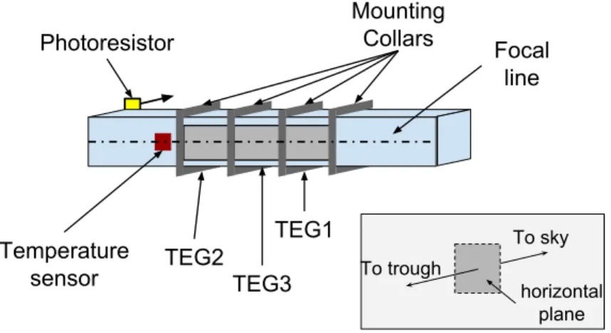
A square aluminum cooling pipe is oriented across the focal line of a parabolic trough. Three thermoelectric devices are fastened with mounting collars to the pipe such that the focal line lies directly across the devices. A pump connected to a DC power supply is used to circulate water (the cooling fluid in this experiment) through the pipe. Figure 1 in the beginning of this report gave a broad view of this experimental set up, while Figure 7 gives a more detailed view, including the sensor arrangements.
Mounting
Collars Focal
line
Temperature sensor
Photoresistor
TEG1 To sky
horizontal plane To trough
TEG2 TEG3
Figure 7: Underside view of sensor and device placement in experimental set up. Note that TEG3 is nested between TEGs 1 and 2.
understand the efficiency of the devices. Furthermore, a photoresistor pointed upwards to the sky is used to give an indication of possible factors (amount of cloud cover) which decrease overall power production. Experimental data is recorded autonomously via a micro controller system. Specifically, analog measurements from the temperature sensor, photo resistor, and voltage measurements from each TEG across its own load resistance are recorded.
Before delving into experimental analyses, it is worthwhile to discuss the selection and justification of this system at hand.
5.2
System Justification
Since the desire here is to explore the renewable nature of thermoelectric devices, an ob-vious source of energy is solar. Hence, a concentrated solar collector is used. Although concentrated solar power is able attain higher temperatures than otherwise possible, it does so passively. Consequently, the hot side temperatures are largely outside of the control of the designer. The designer does, however, have control of the dissipation of the waste heat from the system. Essentially, the dissipation of heat is made easier by indirectly heat-ing the devices. While many researchers prefer to heat the devices indirectly, this system heats the devices directly in an attempt to minimize thermal losses associated with indirect methods. Directly heating the devices in this way requires an immediate cooling system which does not drastically impinge on the energy collected. A solar trough is used here because its linear nature nicely facilitates the use of a running water system to cool the devices.
of choice for many applications. The availability and strength of water make it the clear choice in many cooling situations.
5.3
Equipment
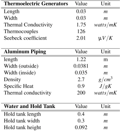
In order to thoroughly explain the experiment, a brief description of the equipment used is given. Herein an approximation of associated measurement error will be also be given. The relevant equipment and parameters are tabulated at the end of this section.
Three 30mm by 30mm power generating thermoelectric devices were used. Specifi-cally, CustomThermoelectric’s 126 couple power generating devices were chosen not only for their reported power output, but also for the completeness of their reference data. Hav-ing access to a complete and thorough data set for these devices will be very useful in evaluating the overall system performance.
The thermoelectric devices were fastened to an aluminum square pipe with aluminum collars. Shims were used to secure the collars in place. Aluminum was chosen for the cooling assembly because of its high thermal conductivity. The purpose of the cooling assembly was to dissipate the waste heat from the cold side to the TEG as quickly and ef-fectively as possible. Thus, aluminum’s high thermal conductivity made it the near perfect material for this purpose.
The parabolic mirror was sourced from a previous project, and provided an accessible structure to base this experiment. A polished stainless steel mirror made the reflecting surface for the parabolic trough. Furthermore, the previous project also provided a low power pump and water hold tank. Parameters for these devices are listed in the following table.
A TMP36 temperature sensor was used to measure the hot side temperatures. This sensor poses the limiting source of error in all measurements for this experiment, with an error of±1.5◦C. Furthermore, a photo resistor was pointed along the axis of the trough towards the sky. This sensor, though it did not give particularly quantitative data, it gave a qualitative measure of the radiation which the array is collecting. Specifically, it was used to account for the weather (clouds) conditions and their effect on the power production.
An Arduino Uno (a rather popular micro controller) was used to continuously and automatically record information about the experiment. For the outdoor experiments the output voltage of each TEG as well as the measurement data from the sensors was mea-sured and recorded every two minutes. Bench top measurements were taken every two seconds. Using this micro controller enabled automatic and consistent data measurement.
5.4
Data measurement methods
Table 2: Equipment Specifications
Thermoelectric Generators Value Unit
Length 0.03 m
Width 0.03 m
Thermal Conductivity 1.75 watts/mK
Thermocouples 126
Seebeck coefficient 2.01 µV/K
Aluminum Piping Value Unit
length 1.22 m
Width (outside) 0.0381 m
Width (inside) 0.035 m
Density 2.7 g/cm3
Specific Heat 0.9 J/gK
Thermal conductivity 200 watts/mK
Water and Hold Tank Value Unit
Hold tank length 0.4 m
Hold tank width 0.3 m
Hold tank height 0.092 m
face of the device. This will of course lead to a reduction in the overall output of this TEG, however power from the other two modules will be unhindered.
Because the TEG modules are affixed directly to the face of the aluminum pipe, it is difficult to place one of the (rather thick) temperature sensors directly on the cold side of one of the TEGs without significantly reducing its thermal contact with the cooling pipe. Though it will not give an entirely accurate reading, the second temperature sensor will be placed on the side of the piping. This is a sacrifice in accuracy of measured data, but other recorded information (such as the output voltage) will be telling of the accuracy of this measurement.
As discussed earlier, the TEGs will produce a maximum power output under load matched conditions. Therefore, to match the internal resistance of the devices, a load of 5-6Ω is required. During testing it is not readily possible to vary the load resistance of
each device according to its current internal resistance. As such, two of the TEGs will operate under a 5Ωload, while the third will have a 6Ωload.
6
Experimental Analysis
per-formed to characterize the behavior of the cooling system. Finally, outdoor experiments were conducted to give an indication of the true performance of the system.
6.1
Modeling Theoretical Performance
6.1.1 Model Formulation
A simplified approach is taken to model the performance of this system. Treating the TEG as a lumped block of material we may use the heat equation to describe the temperatureT
with respect to location in the blockxas
∂T
∂t =
K
ρcp
∂2T
∂x2 +
qv
ρcp
(17)
WhereK,ρ,cp give the thermal conductivity, density, and specific heat of the TEG block
of material. Normally,qv is the heat generated in the material per unit volume. However,
we can instead impose that this term represent the electric power produced by the device. Recall that the electric power generated by the devicePelec is
Pelec=RLI2=RL
mS∆T
R+RL
2
Here, with the block positioned with its hot face atx=0 and its cold face at x=L, then
∆T =T(0)−T(L) where L is the length of the TEG block. While there is some error
involved, the respectively low temperature applications being explored here allow us to safely assume material parametersK,ρ,cp,Sare constant. Setting
α =RL
mS R+RL
2
then we see that
qv= −α
AL (T(0)−T(L))
2
Since we are primarily concerned with the steady state behavior of the system, Equation 17 gives
∂2T
∂x2 =
α
AL(T(0)−T(L))
2
(18)
To a good approximation we can say that the temperature at the end of the device will be equal to the temperature of the water,
T(L) =Tw
Additionally, we can impose a boundary condition on the front face of the device. The flux
Φ(power per unit area) across this boundary will be proportional to the first derivative of
the temperature with respect to position, evaluated atx=0. That is,
−K∂T
∂x
x=0
2 4 6 8 10 12 14 250
300 350 400 450 500 550 600 650
Hotside Temperature (K)
Absorbed Power (W)
TEG2 Hotside Temeprature Dependence on Absorbed Power
(a)
300 310 320 330 340 10
30 50 70 90 110 130 150
Hot Side Temperature (K)
Power ( mW )
TEG2 Modeled Power and Efficiency
300 310 320 330 340
1 2 3 4 5 6 7 8
Efficiency(%)
Electric Power Efficiency
(b)
Figure 8: Model Results for TEG2. (a) shows the near-linear relationship between absorbed power and hot side temperatures. (b) gives the output power on the left and efficiency on the right axis for various hot side temperatures.
The flux across the front boundary is given by
Φ= 1
A(Pabs−Prad)
wherePabs andPrad give the absorbed and radiated heat in watts. The absorbed heat will be taken as a constant and will be given the by the power radiated from the mirror surface. The power radiated from the surface of the TEG, on the other hand, is given by
Prad=ε σAT(0)4
as discussed in previous sections. Generally, since Equation 18 is a second order, ordinary differential equation the solution will have the form
T(x) =C1x2+C2x+C3
Thus, given these boundary conditions, material parameters, and values forTw andPabsit is very straight forward to find the coefficientsC1,C2,C3.
6.1.2 Results
at higher temperatures. This model has been formulated by assuming that the material parameters of the devices remain constant, which is certainly not true at high temperatures. With this in mind, we can use these model results to interpret experimental data.
6.2
Bench top Tests
In order to understand the ultimate efficiency of the cooling system, a series of bench-top tests are required. The thermoelectric devices were supplied with a constant source of heat. Accordingly, the output electrical power of each device was measured for varying water flow rates. These varied flow rates, as discussed in previous sections, directly affect the ability of the system to dissipate cold side waste heat from the devices.
6.2.1 Configuration
TEGs
To hold Tank From hold
Tank
Mounting Collars
Distance to source, d Heat
source
Figure 9: Diagram of bench top testing arrangement to analyze cooling system performance
Referring to Figure 9, a heat gun with a 2.54 cm diameter nozzle was used as a con-trolled and consistent heat source by which the nature of the cooling system could be analyzed. The device was pointed such that the normal line from the nozzle pointed di-rectly in line with the normal of the TEGs along the cooling assembly wall. Using 18◦C
cooling water, the device was positioned 30 mm away from each thermoelectric generator separately. For each generator, voltage measurements are recorded at 2 second intervals for 5 minutes at three possible flow rates.
6.2.2 Radiant Power Calculation
In order to calculate the power incident on the TEGs in this set up, we first treat the heat gun as a blackbody radiator. Then, the emitted power from this sourcePs is
Ps=Asσ(Ts4)
whereTs and As are the source temperature and surface area respectively. The heat qin watts that is radiated onto the surface of the TEG is given by [6] as
The angle between the normal line of the source and that of the receiving surfaceθ in this
case is zero. Furthermore,Ωgives a measure of the relative size of the receiving surface
in relation to its distance from the source. In other wordsΩis the solid angle subtended
by the receiving surface. In the case of a rectangular receiving surface, the solid angle can be calculated as [9]
Ω=4 arccos
s
1+C2
a+Cb2 (1+Ca2)(1+C2b)
!
whereCaandCbrelate the lengthaand widthbof the receiving surface to its distanceD
from the source
Ca=
a
2D ,Cb= b
2D
The load resistance, relative length and width dimensions, calculated input power and the modeled output power for each device are are listed in Table 3. Specifically, the modeled output power here will help to validate the theoretical model of the system. Validation of the model will be critical for interpreting outdoor measurements.
Table 3: TEG calculated absorbed power and model predicted output power
Load Resistance(Ω) a (mm) b (mm) Input Power (Watts) Output Power (mW)
TEG1 6.96 25.1 30 2.002 78.5
TEG2 4.84 26.1 30 2.071 89.8
TEG3 4.74 24.1 30 1.934 78.1
6.2.3 Results
Table 4: Measured electrical power output for various cooling fluid mass flow rates
Flow Rate (g/s) Power, mW (Efficiency, %)
TEG1 TEG2 TEG3
287 106.4 (5.31) 92.6 (4.47) 130.8 (6.77) 340 110.3 (5.51) 93.4 (4.51) 130.3 (6.74) 400 108.3 (5.41) 94.1 (4.55) 129.4 (6.69)
At the onset, one would expect TEG3 and TEG2 to produce near equal power due to their similar load resistances. However, this is not the case. As Figure 10 shows, TEG3 produces much more power than either of the other two devices. This is likely due to the fact that TEG3 is positioned between the others. Being placed in this way, it is possible that the nested device is able to dissipate some of its waste heat to the devices on its perimeter, thus increasing its overall performance.
Furthermore, Figure 10 is ultimately descriptive of the cooling system performance. Recall that TEG1 and TEG2 have load resistances of 6.96Ωand 4.84Ω, respectively. As
0 50 100 150 200 250 300 350 0
20 40 60 80 100 120 140
Time (s)
Power (mW)
Controlled Power Production with 287 g/s Flow Rate
TEG1 TEG2 TEG3
Figure 10: Controlled experiment with consistent heat source. 18◦C water, moving at 0.287 kg/s, is used in the cooling assembly. Electrical power produced across loads of 6.96Ω, 4.84Ω, and 4.74Ωfor TEGs 1, 2 and 3 respectively
under a load resistance which matches its own internal resistance. Here, it seems as though the larger load resistance is better suited for the situation. Because the internal resistance of the device increases with its average temperature, and assuming that the hot sides of each of these devices in nearly the same, then we see that the back side of the devices are not especially cool. However, the cooling assembly does present a unique facet which is critical for power production.
Referring to Table 4, the effects of the flow rate on performance become more no-ticeable. While TEG1 outdoes TEG2 in all cases, each device sees a peak in its own production at different flow rates. TEG1 produces its most power (and most efficiency) with a cooling fluid flow rate of 340g/s while TEG2 peaks at 400g/s. This difference is evidence that the flow rate of the cooling fluid will change the average temperature of the device. Since TEG1 has a larger load resistance it will produce power more effectively when it is hot enough to have its internal resistance match this load. Thus, TEG1 peaks in performance at a slower flow rate. On the other hand, because TEG2 has a smaller load resistance, it requires a lower average device temperature in order to optimally match its respective load, which is achieved by means of a faster flow rate. Here it is clear that this proposed system has the ability to dynamically match its load. Additional figures showing power production for other flow rates can be found in the appendix (Figure 18).
and that the temperature of the water would remain constant. While the water temperature for these experiments did not change dramatically throughout the testing process, however it is clear by 4 that the flow rate of the water has changed the relative back side temperature of the devices. The modeled predictions for TEG1 disagree greatly, and is likely due to the much larger load resistance of the device. TEG3, as discussed above, likely saw an additional effect of absorbed heat that was unaccounted for in the model. Thus, given these caveats, we can make use of the model predictions for the outdoor experiments.
6.3
Outdoor Tests
Several outdoor experiments, using actual solar radiation as the source energy, were carried out. These results give an implication of the working efficiency of this proposed system. Although the previous section has demonstrated the abilities of the cooling system, it is important to analyze the system holistically in order to understand issues which will affect the overall performance. Three key outdoor data sets were collected with the intention of exploring the performance of the system under different settings. For the first two tests data was collected for a two hour span at two different water flow rates. The final test used chilled cooling water in order to examine some extreme potential of the device.
It should be noted that these tests were performed in optimal conditions. These tests were only carried out on particularly sunny days. However, the ambient air temperature, as well as other factors like wind, contribute to non-static results. Although they were not explicitly used in this analysis, photoresistor and focal point temperatures were recorded. This data is presented in Figures 19 -24 in the appendix. They show the degree of variabil-ity in the solar resource even on a fairly clear, sunny day.
6.3.1 Data Collection
In order to observe the long-term results of this system, data was read and recorded from the sensors and TEGs every two minutes. Because of the dynamic nature of the weather, instantaneous readings would vary over time. Thus, taking readings every two minutes demonstrated aggregate behaviors of the system without a cumbersome dataset. In other words, it was unnecessary to see the near instant changes in performance for such a system. What was necessary, however, was data collected over a longer period of time. Here, these experiments were carried out for at least 1 hour, and 2 hours in most cases. These long experiments allow the system to reach, or at least approach, a working steady state.
6.3.2 Incident Power and Efficiency
6.3.3 Results
0 1000 2000 3000 4000 5000 6000 7000 8000
2 4 6 8 10 12 14 16
Time (s)
Power (mW)
Power Output with Cooling Fluid Flow Rate of 287 g/s
TEG1 TEG2 TEG3
(a)
0 1000 2000 3000 4000 5000 6000 7000 8000
2 4 6 8 10 12
Time (s)
Power (mW)
Power Output with Cooling Fluid Flow Rate of 397 g/s
TEG1 TEG2 TEG3
(b)
Figure 11: Two hour spans of data taken on a sunny and windy day. (a) Represents data taken with a 281 g/s cooling fluid flow rate, while data in (b) was measured with a 397 g/s flow rate.
Figure 11 gives the recorded output power for each device with two different cooling fluid flow rates. As was discussed in previous sections, notice that TEGs 2 and 3 out-perform, generally speaking, TEG1 with the faster flow rate. In order to understand the potential of this system in dynamic (real world) conditions, we may look at the upper and lower bounds of power produced.
With a flow rate of 281 g/s, Figure 11a, shows that the power is found almost entirely between 4 and 14 mW. Furthermore the average power produced, across all three TEGs is 7.4 mW per device. While the standard deviation of this data is quite large (2 mW), we see that each device produces between 9.4 and 5.4 mW on average. Additionally, given the formulated model, we can approximate the efficiency of this system. Recall that the model presented a relationship between the output power, efficiency and hot side temperature of a device (as in Figure 8b). Based on these model calculations, each device was operated on the order of 0.5% throughout this experiment.
slightly lower production in comparison to the faster flow rate. Here again the devices operate, by the model formulations, on the order of 0.5%.
0 500 1000 1500 2000 2500 3000 3500 4000 4500
0 5 10 15 20 25 30
Time (s)
Power (mW)
Power Output With Chilled Cooling Water, 287 g/s flow rate
TEG1 TEG2 TEG3
Figure 12: One hour span of data recorded on sunny, calm day with iced water cooling fluid flowing at 297 g/s
In order to explore the potential of this system, an experiment is carried out with ice water as the cooling fluid. In Figure 12 we see that the output is bounded between 10 and 28 mW. On average each device produces between 13.3 and 23.3 mW of power. Based on the model formulations, these devices were normally then operated at roughly 2.5% efficiency.
7
Study Implications and Conclusions
A simple solar concentrating thermoelectric system has been proposed and analyzed. It was supposed that the simplified approach of focusing solar energy directly onto the face of the devices, and cooling them via a moving water system would create a suitable power generation method. A mathematical model was formulated to predict and interpret power outputs for various conditions. Controlled bench top experiments were carried out to not only gage the effectiveness of this model, but also to explore the behavior of the cooing system. First, it was found that the model sufficed, generally speaking, to predict the output power of the devices. Second, the controlled experiments exemplified the effects of flow rate on power output which the model was not able to capture. Most importantly, we saw that larger flow rates were more effective for devices with larger load resistances. Controlled experiments showed efficiencies of 4-7%, while producing 105-130 mW of power for each device. Finally, outdoor experiments were carried out to examine the raw ability of this system. Using the formulated model to infer the working efficiency of the devices, the system was seen to operate at roughly 0.5% efficiency while producing approximately 4-9 mW of power per device.
ideal power could only be produced in the 4 warmest months out of the year (June,July, August, September for North Carolina), then this array would produce 18kWh of power in that time. Alone this power seems fairly significant. However, according [4] , the av-erage person in North Carolina consumed 14,325 kWh of electricity in 2010. Even this relatively small array that we have supposed would cost nearly $4500 for the TEGs alone. With power rates at $0.0967 per kWh, a person would only save approximately $2 on his or her energy bill for those 4 months. At this rate the costs far outweigh the benefits, at least financially. Moreover, the raw outdoor data found in this study even further re-duce the viability of this system. However, with increasing demand for renewable energy sources, the capability of thermoelectric systems is not to be dismissed.
While this study has shown relatively low efficiencies and power outputs, especially for raw outdoor experiments, there are fairly simple adaptations that can be made to improve performance. First, a glass enclosure could be implemented to prevent convective losses to the ambient air. This enclosure would also circumvent any adverse effects caused by windy conditions. Additionally, a selective surface material on the face of the TEGs could be utilized to more efficiently absorb the most energetic wavelengths of light. Lastly, the mounting collars used in this research may have blocked too much incident radiation from the devices. Instead, an alternative mounting method could be used. For example, it may be more beneficial to sandwich the devices between the cooling assembly and a thermally conductive material. Light would then be focused onto the material first, then the heat would be transferred to the TEGs. All together, these measures present interesting cases for further research on this simple system.
Perhaps most interestingly this research has demonstrated the ability of this system in the context of a larger power system. Specifically, it was seen that the mass flow rate of the cooling fluid would match most efficiently to specific load resistances. Thus, such a system could easily be made to meet the dynamic load resistance of a real power grid very efficiently by simply adjusting the fluid flow rate. Although the specific optimal adjustment parameters would need to be studied, this research has demonstrated the ability of this system to achieve maximum efficiency for dynamic loads.
References
[1] Anjaneyulu, Y. Energy Resources: Utilization and Technologies BS Publications, Hyderabad, India. 2012.
[2] Bhandari, C.M.. Thermoelectric Transport Theory. CRC Handbook of Thermo-electrics. Edited by D.M. Rowe. CRC Press 1995.
[3] Calabro, Emanuele.An Algorithm to Determine Optimum Tilt Angle of a Solar Panel from Global Horizontal Solar Radiation. Journal of Renewable Energy. Volume 2013, Article ID 307547. 2013.
[4] California Energy Comission.U.S. Per Capita Electricity Use by State in 2010. En-ergy Almanac.
[5] Decher, Reiner,Direct Energy Conversion: Fundamentals of Electric Power Produc-tion. Oxford University Press, 1997.
[6] Incropera, DeWitt, Bergman, Lavine.Fundamentals of Heat and Mass Transfer. Wi-ley and Sons. 2007.
[7] Joffe, A.F.,Semiconductor Thermoelements and Thermoelectric Cooling. Infosearch Limited, London, 1957.
[8] Lubieniecki, Michal; Uhl, Tadeusz,Thermoelectric Energy Harvester: Design con-siderations for a bearing nodeJournal of Intelligent Material Systems and Structures. 2012.
[9] Mathar, Richard J. Solid Angle of a Rectangular Plate. Max-Planck Institute of Astronomy. February 21, 2014. http://www.mpia-hd.mpg.de/ mathar/public/mathar20051002.pdf
[10] NASA,Multi-Mission Radioisotope Thermoelectric Generator, Space Radioisotope Power Systems. NASA. January 2008.
[11] National Renewable Energy Laboratories, Solar
Radia-tion Data Manual for Flat-Plate and Concentrating Collec-tors.http://rredc.nrel.gov/solar/pubs/redbook/PDFs/NC.PDF
[12] National Renewable Energy Labratories, Solana Generating Station Concentrating Power Projects. 2013.
[13] Pollock, Daniel D.General Principles and Theoretical Considerations. CRC Hand-book of Thermoelectrics. Edited by D.M. Rowe. CRC Press 1995.
[15] Rowe, D.M.IntroductionCRC Handbook of Thermoelectrics. Edited by D.M. Rowe. CRC Press 1995.
[16] Shakouri, Ali; Yazawa, Kazuaki,Scalable Cost/ Performance Analysis for Thermo-electric Waste heat Recovery Systems. Journal of Electronic Materials. V 41 N 6, pp 1845-1850. 2012.
[17] Stevens, James W.Heat Transfer and Thermoelectric Design Considerations for a Ground-Source Thermoelectric Generator. 18th International Conference of Ther-moelectrics 1999.
[18] Stine, Geyer. Power From the Sun Online Resource. Adapted from Solar Energy Systems Designby Stine and Harrigan. 2001.
[19] Teutsch, Werner B,Some Considerations of the Basic Physics of Thermoelectric Ef-fects. In Thermoelectricity. Edited by Egli, Paul H. 1960
[20] TXL Group, Ultra-Low Voltage Bootstrap Converter ELC-W0422-1/2 Datasheet. Custom Thermoelectric LLC. 2012.
[21] University of Pensylvania, School of Engineering and Applied Sci-ence. Correlations List: External Free Convection Correlations. http://www.seas.upenn.edu/ meam333/correlation/CorrelationsList.pdf 2013.
Appendix Figures
2 4 6 8 10 12 14
250 300 350 400 450 500 550 600 650
Hotside Temperature (K)
Absorbed Power (W)
TEG1 Modeled Hotside Temepratures with Tw = 274 K
(a)
300 310 320 330 340 10 30 50 70 90 110 130 150
Hot Side Temperature (K)
Power ( mW )
TEG1 Modeled Power and Efficiency at Tw = 274 K
300 310 320 330 340
1 2 3 4 5 6 7 8 Efficiency(%) Electric Power Efficiency (b)
Figure 13: Model Results for TEG1 with 293 K cooling water. (a) shows the relationship between absorbed power and hot side temperatures. (b) gives the output power on the left and efficiency on the right axis for various hot side temperatures.
2 4 6 8 10 12 14
250 300 350 400 450 500 550 600 650
Hotside Temperature (K)
Absorbed Power (W)
TEG3 Modeled Hotside Temepratures with Tw = 274 K
(a)
300 310 320 330 340 10 30 50 70 90 110 130 150
Hot Side Temperature (K)
Power ( mW )
TEG3 Modeled Power and Efficiency at Tw = 274 K
300 310 320 330 340
1 2 3 4 5 6 7 8 Efficiency(%) Electric Power Efficiency (b)
![Figure 2: Thermodynamic circuit to explain Seebeck, Peltier and Thomson effects. Pollock’s work [13].](https://thumb-us.123doks.com/thumbv2/123dok_us/8333748.2211573/8.918.148.732.119.243/figure-thermodynamic-circuit-explain-seebeck-peltier-thomson-pollock.webp)