Evolving Relationship between Oil and
Corn under Structural Changes
Final Honors Thesis
Zijun Tian
March 06, 2017
Economics Department
University of North Carolina at Chapel Hill
Thesis Advisor: Dr. Peter Hansen
Faculty Advisor: Dr. Klara Peter
Approved:
Abstract
This paper focuses on the better estimation of the correlation between oil and corn with Realized Beta GARCH model, the first moment Granger Causality test on the prices of oil and corn, and the second moment causality test on the volatilities and returns of oil and corn. Since the past decade has witnessed the ever-fast development in biofuel production and increasing volatilities in the markets, I further perform Bai and Perron Procedure to detect possible structural breaks from 2004 to 2014 and use impulse response functions to help draw insight into the changing causal relationships in the price levels. I find that the correlation between oil and corn nearly doubled during the financial crisis and then resumes back to the normal level about 0.2. However, the statistically significant causal relationship from oil prices to corn prices detected in the prior crisis period cannot be found later as a result of higher volatilities and nonexistent arbitrage. The second moment causality test on the
Acknowledgement
I. Introduction
The relationship between crude oil and agricultural commodities has changed dramatically over the past decade, increasingly affected by the development of renewable energy, and turbulent financial market. Since biofuel, substitutable for crude oil, has been more widely accepted by consumers and supported by government, we may expect evolving relationship between oil and agricultural commodities, especially for those used in the production of biofuel. Based on the primary and wide use of oil in the agriculture production and the most technically obtainable and mature substitution between oil and ethanol that heavily depends on the corn as the input, this paper addresses the recently accelerated trend of corn’s
emergence as an energy crop and the complicated oil-ethanol-corn relationship.
According to United States Department of Agriculture Economic Research Service, US has a dramatically rapid growth in the share of corn use for fuel ethanol in the last few years. Three or four years ago, the share only accounted for 12 to 14 percent of total U.S. corn use.
However, under current conditions, ethanol share in the total corn use accounts for about one third of the total demand for corn in U.S. and is expected to further increase in the next few years with government mandates that call for increased ethanol use. With the help of increasing demand of corn in the energy market that is second in size only to the demand in the domestic feed market, the agricultural production of corn in U.S. has survived from excessive production capacity, low prices, and heavy dependence on government income supports and becomes an ever-growing sector with frequent periods of tight supplies and food price surge. On the one hand, the sizeable increase in ethanol use of corn tends to
various sectors such as consumers, crop and livestock farmers, renewable energy industry, and traditional energy market.
Therefore, the degree of stability and strength of the relationship between oil and corn plays an important role in appropriate risk-management strategies as well as an insight into the consumption behaviors and investment plans. Four major research papers have explored the correlation between oil and corn. Tang and Xiong (2012) analyzed the increasing correlation between oil price and other non-energy commodity prices by focusing on the index
investment and financialization in commodity markets. Along the similar line, Thorp (2015) also argued that the correlation between oil and most agricultural commodities returns has been markedly increased and become more volatile and conducted impulse response function analysis among crude oil and three major agricultural commodities including corn, wheat, soybeans. In addition to an integrated partial equilibrium framework that showed the impact of ethanol promotion on the correlation between oil and corn (Tyner and Farzad, 2008), more advanced time series econometrics may draw new insights into this relationship. By applying both discrete and smooth threshold error correction models, Merkusheva and
having less attention and exploration, can provide us with a step-ahead forecast of the prices and volatilities of oil and corn. In order to draw more insight into the causal relationship between oil and corn and explain certain phenomena happening in more economically disturbed periods that we cannot easily interpret based only on Granger causality test results, I also conduct an analysis of impulse responses to examine how the change in the percentage change of prices of each commodity in the system responds to one standard deviation shock of the other. Finally, I also explore possible explanations for the observed changes in the correlation and causalities between oil and corn corresponding to the detected structural breaks including policy, agricultural, and financial causes. Due to the more volatile financial market after financial crisis in 2008, I hypothesize that the correlation between oil and corn significantly increases afterwards. Additionally, based on the more exogenous supply of oil and the high volatility of its prices, I may expect that the first moment causality of price levels goes from oil to corn. However, it is highly possible that the causality is spurious and the market prices of these two commodities are not causally related since both prices are volatile and not very predictable. Under this consideration, I may rather hypothesize that the causal relationship from the returns of oil to the volatilities of corn is significant,
corresponding to Merkusheva and Rapsomanikis’ analysis using error correction models (2012).
crisis period even after financial crisis, which corresponds to the lack of arbitrage in the financial market. With regards to the corn price shocks presented in Figure 5 b), 6 b), 7 b), 8 b), the initial response of the percentage change of oil prices is not significant under the full dataset as well as in each regime, corresponding to no significant causal relationship from corn prices to oil prices. The abnormality of Figure 9 b) will be explored in details later. However, Figure 5 c) and 6 c) confirms the inverse causality since the initial response of the percentage of change of corn prices to the oil price shocks is positive while significant and the latter, or the first sub-period, has larger magnitude and smaller variances. If we look at the causality from the perspective of volatilities and returns where nonstationarity in the prices are eliminated, we can detect a significant causal relationship that the returns of oil at time t-1 can help predict the volatilities of corn at time t at significance level 0.05.
This paper unfolds as follows. Section 2 presents a literature review of the past theoretical techniques and empirical analysis. It also contains the potential contribution of my research based upon its extension from the previous works. Section 3 introduces the basic theoretical model I plan to use. Empirical model and general methodology are outlined in Section 4. Section 5 contains data selection and modification, and we discuss our results and findings in section 6, followed by conclusions in Section 7. All tables and figures are collected in the appendix after Section 7.
II. Literature Review
GARCH model by incorporating realized measures and leverage functions. In order to better estimate the dynamics between the market return and an individual asset return, they
proposed Realized Beta GARCH model that extracts information from realized variances and covariances to calculate conditional correlation. Secondly, Tang and Xiong (2012) analyzed the increasing correlation between oil price and other non-energy commodity prices by focusing on the contemporaneous increasing trend of index investment in commodity markets. In particular, they demonstrated that the recent higher correlation between oil price and other indexed commodities prices are concurrent with more investment in these
commodities. Thorp (2015) also argued that the correlation between oil and most agricultural commodities returns has been markedly increased and become more volatile. She admitted the existence of structural changes in conditional correlation that can occur at the time of the introduction of biofuel policies. Additionally, based on her analysis of impulse responses, Thorp noted that the adjustments to the oil price shocks is stronger for biofuel feedstocks, like corn, and negligible for many other agricultural commodities, which suggests that the substitutability between biofuel and oil, and the reliance of the production of biofuel on agricultural commodities play an important role in driving the binding relations. With one step ahead, Merkusheva and Rapsomanikis (2012) analyzed the nonlinear linkage between oil, ethanol and other grains prices in the short run. In the long run, as they suggested, oil prices are the drivers of ethanol and grains prices, and they adjust to the small deviations of oil price very quickly.
However, while most of the literatures have been focused on the correlation between oil and corn, the models by which they calculate the correlation are less accurate and less
returns that are the return of oil and the return of corn to calculate their correlation.
Additionally, the economic analysis on the causality between oil price and corn price is much more scarce and usually absent, not to mention the causality between the volatilities and returns of oil and corn. Without being aware of the causal direction between the prices of these two goods, policy makers may not be able to determine what the impact of biofuel policies on the oil market might be or whether these policies can bring potentially adverse fluctuations in the oil market. Without having sensible and relatively accurate prediction of the range of changes in which these two goods’ prices can bring, governments may not be able to adopt an effective risk management approach. Firms may only have limited planning horizons, leading to investments postponement and expensive reallocation of resources. Economists also need forecasts on macroeconomic trends and risk exposure of energy and agricultural commodity markets. For example, it is crucial for them to know if an oil shock will influence biofuel market at first, the demand for corn subsequently, and the price of food that is relevant to each individual consumer eventually.
III. Theoretical Model
Under the assumption of competitive retail energy and agricultural commodities markets, my theoretical models are the basic economic models of supply and demand, and substitutes and complements proposed by Alfred Marshall in his work Principles of Economics in 1890. Since the number of sellers is sufficiently large and there are generally no barriers for new firms to enter the market, we can reasonably assume that the markets are perfectly
and volatility changes but cannot easily determine the underlying sequential dynamics between them. There is no denying that the casual relationship between oil and corn can take many forms.
Modern agriculture uses oil products to fuel farm machinery, to transport raw input to the farm, and to transport farm output to the ultimate consumer. Additionally, oil is often used as input in production of agricultural chemicals. Therefore, oil price increases put pressure on the supply of agricultural commodities, like corn. Decreasing supply of corn drives up its price in the market, and thus reflects causality from oil price to corn price. This causal direction may also build upon the relationship between corn and ethanol that is the most common type of biofuel. Since biofuels are the only non-fossil liquid fuels able to replace petroleum products in existing combustion engines and motor vehicles, (Thorp, 2015), as oil prices rise, the demand for these alternative fuels will increase, leading to an increase in the demand of corn that is the major feedstock for ethanol. Therefore, corn prices are forced upward. However, the above causality can be reversed. For example, the technological and government mandated expansion of ethanol industry is believed to have contributed to the recent increase in commodity prices. As the price of corn increases, marginal cost of biofuel production also rises. If we assume the market of biofuel is perfectly competitive, then the increase in the biofuel price makes consumers substitute away from now relatively more expansive energy source back to oil. As the demand of oil increases, the price of oil increases correspondingly. Moreover, the causality can also be bidirectional. Some shocks in the macroeconomic environment may impact both prices. One notable instance is the financial crisis in 2008. As a result of wealth effect, when people have less purchasing power, they consume less. Thus, the demand for both energy sources may decrease, leading to
to note that the causality can be asymmetric depending on the current prices of oil and corn, and their respective change rate. In Figure 1, we can observe both similar moving direction and discrepancies between the oil and corn prices. However, when both corn and oil have high prices or their prices are being driven up, their price co-movement is relatively stronger and more obvious.
Additionally, there are also various possibilities and ambiguities in the causal relationship between the volatilities and returns of oil and corn due to the substitutability between and the nature of perfectly competitive market of these two goods. Actually, driven by changes in uncertainty related to supply, demand, and inventories, changes in volatility are extremely crucial for speculation and market stability if we do not assume a rational expectations world. Volatility often reflects the amount of market uncertainty or risk about the size of changes in a commodity’s value. A higher volatility means that a commodity’s value can potentially be spread out over a larger range of values, resulting from changes in market demand, the
release of new economic or supply information, changes in consumers’ expectations, changes in market tastes, or unanticipated events and circumstances that can cause large price
adjustments. Since the changes in market supply and demand of corn can affect those of oil and vice versa, it is hard to determine whether knowing the changes of price of corn can help predict the volatility of oil beforehand or the causality should be the other way around. On the one hand, along with more necessity and awareness of resource scarcity and
relatively more exogenous, supply shocks in oil can lead to changes in the demand of its substitutes, biofuel like ethanol, dramatically, thus leading to the changes in the demand of corn used in energy production. The corn volatility can be driven up even if the initial shock starts in the oil market. However, it may also turn out to be that other unanticipated events can cause the simultaneous increase in the volatilities of oil and corn since 2004. For example, the financial crisis, which initially disrupted the markets for mortgage-backed securities, negatively impacted the balance sheets of many financial institutions. Eventually it reduced the risk appetite of investors for seemingly unrelated assets in their strategic portfolio allocation to avoid more potential uncertainty. The sudden change in market tastes and
demand may lead to the contemporary high volatilities of oil and corn.
Therefore, based on the interaction and variety of the above channels provided by basic economic models of supply and demand and substitutes and complements, it is difficult to tell from rule of thumb if there exists a causal relationship that can help us predict the volatility of one commodity using the price information of the other without further analysis. If there does exist such a way, then I aim to find out what direction and to what level of that causal relationship actually is.
IV. Empirical Model
4.1 Bivariate Realized Beta GARCH model
The ordinary least squares model assumes that the expected value of all squared error terms is the same at any given point. However, since the accuracy of the predictions of financial asset is important for portfolio selection, risk analysis, and derivative pricing, we need to
variance of the error terms larger for some ranges of data than for others. Therefore, we need models, like GARCH (generalized autoregressive conditional heteroskedasticity), which are capable of treating the undesired heteroskedasticity as the variance to be modeled instead of trying to avoid and fix it as what the OLS model does. From this point view, even if “robust standard errors” (Engle, 2001) makes the concern over heteroskedasticity less problematic, our requirement for model accuracy and for the insight of the variance changes of the error terms make the basic version of the least squares model relatively inapplicable and biased. Thus, I use Bivariate Realized Beta GARCH model, an improved version of GARCH model, which incorporates current levels of volatilities and correlation to calculate both the
conditional variance and conditional correlation between oil and corn of a ten-year timespan. Lag one is used for both assets because it is the common way used in previous papers. We have five observable variables in the model and we define the information set to be
(r!"#,!,r!"#$,!, x!"#,!, x!"#$,!, y!"#,!"#$,!) where r!"#,! is the realized return on oil, r!"#$,! the realized return on corn, x!"#,! the realized measure of oil volatility, x!"#$,! the realized
measure of corn volatility, and y!"#,!"#$,! the realized correlation between oil and corn. Motivated by findings in the research of Hansen, Lunde, and Voev (2013), we define
z!"#,! ~ i.i.d.N 0,1 and z!"#$,! ~ i.i.d.N(0,1). Furthermore, as it states in Andersen et al.
(2001b), returns standardized by realized volatility are approximately normally distributed. Therefore, if we define h!"#,! and h!"#$,! to be conditional variances of oil and corn
respectively at time t, then we have r!"#,!= µμ!"#+ h!"#,! z!"#,! and r!"#$,!= µμ!"#$+
h!"#$,! z!"#$,! that follow our assumptions mentioned previously. If we look at the above
the basic structure of bivariate realized Beta GARCH model that consist of GARCH equation and measurement equation for each individual asset, specifically oil and corn here, we define the model as follows:
log ℎ!"#,!=𝑎!"#+𝑏!"#log ℎ!"#,!!!+𝑐!"#log 𝑥!"#,!!!+𝜏!"#(𝑧!"#,!!!)
log 𝑥!"#,!=𝜉!"#+𝜑!"#log ℎ!"#,!+𝛿!"# 𝑧!"#,! +𝑢!"#,!
log ℎ!"!",! =𝑎!"#$+𝑏!"#$log ℎ!"#$,!!!+𝑐!"#$log 𝑥!"#$,!!!+𝑑!"#$logℎ!"#,!+𝜏!"#$ 𝑧!"#$,!!!
log 𝑥!"#$,!=𝜉!"#$+𝜑!"#$log ℎ!"#$,!+𝛿!"!" 𝑧!"#$,! +𝑢!"#$,!
According to Andersen et al. (2001a, 2001b, 2003), we assign Gaussian specification for
𝑢!"#,! as well as 𝑢!"#$,! such that 𝑢!"#,! ~ i.i.d.𝑁 0,𝜎𝑜𝑖𝑙2 and 𝑢!"#$,! ~ i.i.d.𝑁 0,𝜎𝑐𝑜𝑟𝑛2 .
𝜏!"# z!"#,!!! and τ!"#$ z!"#$,!!! are leverage functions that model the leverage effect of the
dependence between an asset’s return and its changes of volatility. Hansen, Lunde, and Voev justified in their research (2014) that they are basically second-order polynomials. Finally, the equation for the dynamic modeling of conditional correlation between oil and corn is given by
𝐹 𝑦!"#,!"#$,! =𝛏!"#,!"#$+ 𝜑!"#,!"#$𝐹 𝜌!"#,!!"#,! +𝑣!"#,!"#$,!
𝐹 𝜌 is the Fisher transformation that maps the correlation originally ranging from −1 to 1 to
the whole real number line, which spreads out the distribution of correlation and enables us to
observe its changes over time more easily and obviously. Additionally, it also makes
𝑣!"#,!"#$,!~𝑁 (0,𝜎𝑜𝑖𝑙,𝑐𝑜𝑟𝑛2 ) a reasonable assumption. Using log likelihood function and
substituting h! for variance in the normal likelihood, we can have a systematic way to adjust
all parameters simultaneously and give the “best fit” estimation. With all the parameters estimated and known, we can construct time series of conditional variances of oil and corn,
(1)
(2)
(3)
(4)
and the conditional correlation between them. The preliminary estimation results are shown in Figure 2, 3, and 4. Based on the fact that z!"#,! ~ i.i.d.N 0,1 ,z!"#$,! ~ i.i.d.N(0,1), and
the basic property of bivariate normal distribution, we have
E[z!"#,!|z!"#$,!] =𝜌!"#,!"#$,!×z!"#$,!
Therefore, having better estimation of the correlation and knowing z!"#$,! which can be
obtained from the above model, we can know the expectation of the conditional value z!"#,!.
Based upon that, we can further get a contemporaneous intuition on the volatility, or the risk,
of oil.
4.2 Bai and Perron procedure
For the bivariate realized Beta GARCH model established for the volatility and correlation mentioned above, it describes a dynamic process that counts for continuous changes in the market and economic environment. Since domestic policies, international trade pattern, and other supply and demand shocks can influence the relationship between oil price and corn price, it may also be appropriate to model the prices in the same way that includes changes over time. However, currently, their higher volatility and much more unpredictability prohibit us from doing so. Therefore, in order to incorporate underlying changes as well as model much as possible, we rather try to find discrete changes for oil and corn prices, analyzing different regimes instead of full dataset under the assumption of no structural changes. Even if prices are not very likely to jump from one pattern to another, it is still meaningful for us to do so because they allow us to see which event coincides with which breaks and which kind of events, political or economic, internal or external, are more likely to cause huge changes in the prices of oil and corn. The methods of detecting and estimating structural breaks are diverse and have evolved toward more complexity and more applicability. The classic Chow
Test can only test for one structural change with known break point. It simply tests for
whether the coefficients before and after the break are the same, and we can conclude that the given break does exist if we have sufficient evidence to statistically significantly reject the null hypothesis. Then Andrews proposed SupW tests (Andrews, 1993) that allows for detection of a single yet unknown break point within a given time interval of all candidate break dates. Its limitation on the requirement that all the regressors in the ordinary least squares regression must be strictly stationary is later expanded by Fixed Regressor Bootstrap procedure. However, since we can neither tell the number of breaks for sure nor arbitrarily assign an exact number of breaks to the oil and corn prices from 2004 to 2014, we use more advanced Bai and Perron procedure (2003) with full structural model where all parameters are subject to shifts. It is used to detect multiple endogenous structural changes and help split data correspondingly. Basically, this procedure is an iterative method using OLS and allows for general forms of serial correlation and heteroskedasticity in the errors. It is also less restrictive on the distributions of independent variables and errors. They can have trend or even different distributions across segments. Consider the following regression with 𝑛 breaks or, namely, (𝑛+1) regimes:
𝑦!= 𝑧!!𝛼!+𝜐!;𝑡= 𝑇!!!+1,…,𝑇!;𝑗 =1,2,…,𝑛+1;𝑇! =0,𝑇! = 𝑇
Let 𝑦 denote corn prices and 𝑧 denote regressors such as oil price, U.S. ethanol price, inflation rate as a proxy for general market condition, cross-price elasticity of demand between oil and corn that approximates their substitutability, ethanol share in the total use of corn, and wheat price with 𝛼! representing the regime-specific vector of coefficients. We
have 𝜐! to be the disturbance. The method of estimation, according to Bai and Perron, is
based on the least-squares principle. For each n−partition (𝑇!,𝑇!,…,𝑇!), denoted 𝑇! , we
estimate the parameter vector 𝛼! by minimizing sum of squared residuals:
[ 𝑦!−𝑧!!𝑎! ]!
!!
!!!!!!!!
!!! !!!
over all possible partitions of the whole timespan with a maximum number of breaks 𝑢 and minimum regime length 𝑑. In other words, we should satisfy 𝑗 ≤𝑢 and 𝑇!−𝑇!!! ≥𝑑. Then
let
𝛼({𝑇
𝑗}) denote the estimated coefficients and 𝑆!(𝑇!,𝑇!,…,𝑇!) the resulting sum ofsquared residuals. Substituting
𝛼({𝑇
𝑗}) into the objective function of least-squares, we canobtain the estimated break points (𝑇!,𝑇!,…,𝑇! ) such that
(𝑇!,𝑇!,…,𝑇! )= argmin!!,!!,…,!!𝑆!(𝑇!,𝑇!,…,𝑇!)
After obtaining the number and the position of the breaks, we can do separate tests on different regimes and see which events coincide with which breaks.
4.3.1 Granger Causality Test for Price
Granger causality tests on whether oil price is able to increase the accuracy of the prediction of corn price with respect to a forecast based on only past values of corn price and vice versa. It is based on two properties of causality. First, the future cannot cause the past. Second, a cause contains unique information about an effect that is not available or replicable elsewhere. Therefore, we can establish the following inequality:
𝐹 𝑋!!! 𝛺! ≠𝐹 𝑋!!! 𝛺!−𝑌!
where 𝐹 is the conditional distribution; 𝛺! is the information set used to predict 𝑋!!! at time 𝑡; 𝛺!−𝑌! is all the information in the universe used to predict 𝑋!!! except for series 𝑌!.
If the above relation holds, then 𝑌! is said to “granger cause” 𝑋! since it can help predict
future X. For the simplicity of use and interpretation, I establish the vector autoregressive (10)
(8)
(11) (VAR) model and first consider bivariate Granger Causality test where oil price and corn price are the only two variables included in the test, which can be expressed as following:
𝑃!"#,! = 𝛼!+ ! 𝛽!
!!! 𝑃!"#,!!! + !!!!𝛾!𝑃!"#$,!!! +𝜇!
𝑃!"#$,! = 𝜃!+ !!!!𝜑!𝑃!"#$,!!!+ !!!!𝜋!𝑃!"#,!!!+𝜐!
Based on this test and particularly straightforward for the bivariate case, we can have four possible outcomes that depend on ! 𝛾!
!!! and !!!!𝜋!, which are unidirectional Granger-causality from price of oil to price of corn, unidirectional Granger-Granger-causality from price of corn to price of oil, bidirectional causality, and independence between price of oil and price of corn. For example, if !!!!𝜋! is statistically significantly different from zero and ! 𝛾!
!!! is
not, then we can conclude that it is the first outcome. However, the causality may not be limited only to bivariate case since it is hard to define and measure 𝛺! in practice. The
unobserved common factors are always a potential problem for any finite information set. Other factors, like the cross-price elasticity of demand between oil and corn, the fraction of total consumption of corn used for energy use, the price of wheat, and the financial market fluctuations, may also influence the causality between oil price and corn price. Therefore, many efforts have been done on extending the Granger Causality test to a multivariate case. Caines, Keng and Sethi (1981) proposed a reasonable procedure. If a process 𝑋! has more than one causal variable, say 𝑌!,𝑌!,…,𝑌!, we construct bivariate VAR model with each pair of (𝑋!,𝑌!), for 𝑖=1,2,…,𝑛 with order selected to minimize prediction error. Then we rank these causal variables according to a decreasing order of their specific gravity, the prediction error. For each causal variable, the lag order is determined by establishing the optimal
univariate AR model with minimal prediction error. Finally, we add the causal variable one at a time based on their causal rank obtained before with orders optimized at each step. The final result would be an optimal ordered multivariate AR model of 𝑋! including all the causal
variables. However, while we respect all the changes and improvement conducted on the conventional Granger Causality Test, we do believe that simplicity is also important.
Actually, I highly doubt the existence of the first moment (price levels) causality between oil and corn, at least after around 2008 when commodities have been more financialized and more frequently traded in the financial market. Otherwise, there would be huge amount of arbitrage from which speculation can make a lot of money. It is also the reason that I perform second moment (volatility and returns) causality test as well since it may offer more stable and accurate insight on the causality between oil and corn.
4.3.2 Impulse Response Function based on VAR Model
Impulse response functions describe the dynamic response of one variable to a one-period shock from the other variable based on a VAR system that includes stationary variables or time series with time invariant expected values, variances, and covariances. Following the above Granger causality test for the price levels of oil and corn, we want to further analyze how one commodity adjusts to the exogenous shocks of the other. If the response is
statistically significantly different from zero, meaning the 95% confidence interval does not contain zero response, then we can, on the one hand, conclude the unidirectional causality. On the other hand, we can get a quantitative measure of the speed of adjustment of a good to its own shock or to the other good’s shock. Similarly, we consider the whole timespan as well as the four sub-periods corresponding to the three structural breaks we identified via Bai and Perron Procedure previously.
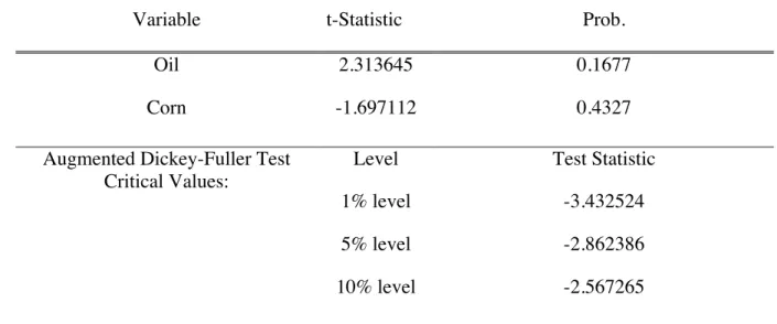
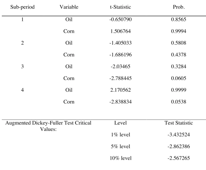
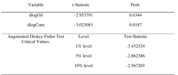
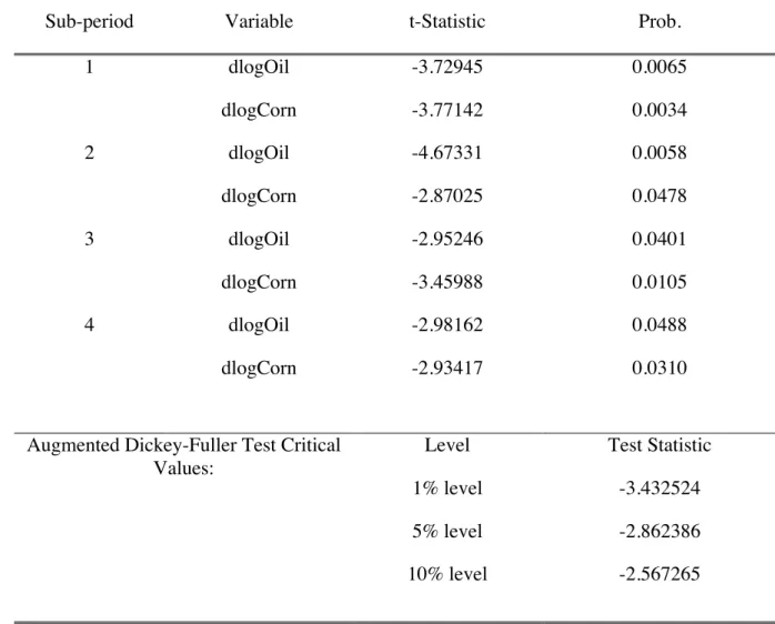
Merkusheva and Rapsomanikis used in their paper (2012). Since the null hypothesis under this test is nonstationarity, we should further transform the variables if we do not have sufficient evidence to reject the null hypothesis at a significance level of 0.05. Based on previous literatures and economic intuition on the price levels’ random-walk behaviors, oil and corn prices are very likely to be the time series of order one. Therefore, we take the log of each of the prices and then take the first difference. Let dlogOil and dlogCorn denote the first differenced log prices of oil and corn respectively. Then we redo the ADF unit root test and stationarity can be reasonably assumed this time with p-value less than 0.05. Further following Merkusheva and Rapsomanikis’s paper on the selection of optimal lag in VAR model, we apply Bayesian Information Criterion (BIC) to select the optimal lag length and ensure the residuals to be white noise. Let p denote the optimal lag. Then the VAR (p) model is as following:
𝑦! =Φ!+Σ!!!!Φ!𝑦!!!+ℇ!
where y! is a 2×1 vector of approximate percentage change of oil and corn prices at time t from time t-1, Φ! a 2×1 vector of constants, Φ! a 2×2 matrix relating the percentage price changes at lagged i period to current percentage changes, and ℇ! a 2×1 vector of i.i.d. vector of constants error terms. More specifically, based on the property of VAR model, each of the two variables is a function of p lags of both variables, including itself, a constant term and a contemporaneous error term. Since we use Cholesky decomposition for the orthogonalized impulse response function that is most commonly used in the previous literatures involving impulse response function analysis, the above equation can be rewritten into a vector moving average (VMA) representation as following:
𝑦! =𝜓!+Σ!!!!ψ
!+ℇ!!!
where ψ! is a 2×2 matrix with each element to be the impulse response with respective to the shock in each variable’s error term.
(13)
4.3.3 Causality Test for Volatility Based on Bivariate Realized Beta GARCH Model
Different from Granger Causality Test for price, we extend the realized Beta GARCH model established before to test for causality in the volatility. There are two reasons for the change of model. First, it allows us to take other factors that may potentially impact the causality between oil and corn into consideration without bothering complicated multivariate test. Second, the realized Beta GARCH model provide us with the most accurate model in
estimating and forecasting the dynamics between oil and corn by continuously incorporating leverage functions that can model the dependence between returns and volatility, and realized measures available in the market. Basically, we reuse the following two equations and add term x!"#$,!!! in the first equation and x!"#,!!! in the second equation:
log h!"#,! =a!"#+b!"#log h!"#,!!!+c!"#log x!"#,!!!+𝑑!"#log 𝑥!"#$,!!!+τ!"#(z!"#,!!!)
log ℎ!"#$,! =𝑎!"#$+𝑏!"#$log ℎ!"#$,!!!+𝑐!"#$log 𝑥!"#$,!!!+𝑑!"#$logℎ!"#,!+
e!"#$log𝑥!"#,!!!+𝜏!"#$ 𝑧!"#$,!!!
Lag one is chosen as given according to Hansen, Lunde, and Voev’s (2014). If e!"#$ can be shown against zero, then we can conclude that the returns of oil can help predict the volatility of corn one time period ahead, specifically one day ahead in this research. Namely, the size of changes associated with corn prices can be explained by the price changes of oil in the previous day, which describes the second moment causality. We can also test
𝑑!"#log𝑥!"#$,!!! similarly in the first equation to see if it is possible that the returns of corn
today can contribute to the oil volatility forecast tomorrow. However, if we do not detect any meaningful causality from the above model, it does not necessarily mean that there does not exist one. Actually, without including other variables relevant to the causality, the test may not be very comprehensive. Therefore, we also include the returns of ethanol denoted by
(15)
𝑥!"!!"#$,! that is the most typical biofuel and the returns of wheat denoted by 𝑥!!!"#,! that is
substitutable for corn in both energy production and food consumption. The reason that we use returns instead of prices is that the stationarity of the model requires stationary process. Prices are not qualified but returns can be better assumed to be stationary. Finally, we use log likelihood maximization again to estimate the coefficient vector and see if any of returns as well as other relevant variables can contribute to the prediction of the volatility. The significance of the estimated coefficients e!"#$ and 𝑑!"# can be obtained through the
comparison between the change of log likelihood and the critical value 𝜒!,!!.!" where n is the
number of constraints in the equation. For example, if we want to test whether e!"#$, the coefficient of log𝑥!"#,!!! in the GARCH equation of corn, is statistically significant, we first
restrict 𝑑!"# to be 0. Then we conduct log likelihood maximization and take the difference between it and the previous log likelihood. Then we compare the change in log likelihood with the value of 𝜒!,!!.!". If it is larger than 𝜒
!!,!.!", then we can reject the null hypothesis that have sufficient evidence to conclude that the returns of oil at time t-1 can help predict the volatility of corn at time t at significance level 0.05.
V. Data
Energy Information Administration and corn price obtained from Farm Journal. They are also adjusted according to the elimination of trading days in the previous dataset. Other relevant variables, including inflation rate represented by CPI (Consumer Price Index), and ethanol share in total use of corn, are monthly data. Without the use of mixed frequency, I can either aggregate daily data into lower monthly frequency or disaggregate monthly data into higher daily frequency. The former one is quite simple because we only need to average the daily data values over a month to convert the data from daily frequency to monthly frequency. The latter one is much more complicated because new method is required. Since we want to keep the daily price variation in the corn and oil price as what they originally have, we use Chow-Lin procedure to disaggregate monthly data, which is proposed and used in previous paper (Chow, Lin, 1971). It basically disaggregate and interpolate a relatively low frequency (monthly) time series to a relatively higher (daily) frequency time series, where either the sum, the average, the first or the last value of the resulting high frequency time series is consistent with the original low frequency data. The cross-price elasticity of demand between oil and corn is also monthly data and need to be converted to daily frequency series. More importantly, we do not have direct data on the elasticity itself. However, based on the
definition of cross-price elasticity of demand and available data on ethanol price and oil sales, we can derive it from the ratio of percent change in quantity demanded of oil to the percent change of ethanol price. However, since the elasticity is derived under the “ceteris paribus” assumption and we do think that in the realistic market, supply side changes do exist, we should be very critical and skeptical toward this derived measure.
VII. Results and Findings
correlation maintains at around a level of 0.2 before 2008 and after 2012. During the middle period, the correlation doubles and fluctuates more frequently, which can be contributed to many events and changes such as financial crisis, surge of commodity prices and
implementation of EISA (Energy Independence and Security Act) of 2007. From Bai and Perron procedure, we obtain that the optimal number of break dates that indicate significant structural changes is three since it has both the largest scaled F-statistic and the largest
weighted F-statistic. The first break date is estimated to be April 01, 2008 that corresponds to the start of the Great Recession from 2008 to 2012. The second one is Oct 08, 2010 that
marks the ever faster development of biofuel production and it is during 2010 that U.S.
became the largest net exporter of ethanol in the world. At the same time, the price of corn
started to increase and reach its peak. The third one is May 13, 2013 that coincides with the
U.S. largest annual increase in oil production. During the same period, transportation
efficiency has been fairly improved, relatively decreasing the demand of oil per vehicle per
mile. These two phenomena combined can partially explain the decreasing trend of the oil
price in the first half of 2013 and the sharp drop throughout the entire year of 2014. Based
upon the fact that the past decade has witnessed a large amount of economic fluctuations and
market changes, it is not surprising that our first Granger Causality test under full dataset is
not very significant. Since the supply of oil is more exogenous, the causality is supposed to
go from oil price to corn price, if there exists one. However, from the results, we can only see
that when lag is limited to 1 or 2, the causality from oil price to corn price is weakly
significant at the 0.05 significance level. Thus, it is necessary for us to do separated tests for
different regimes endogenously determined by BP procedure.
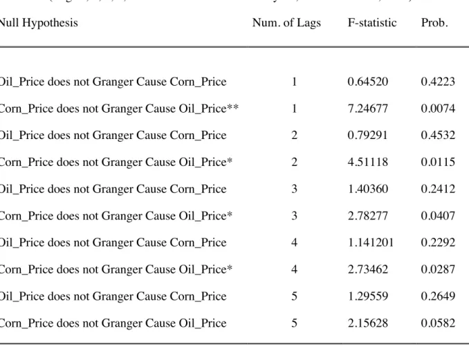
In the first regime, as we can see from Figure 1, oil price and corn price are both relatively
low and no obvious co-movement between them can be detected. More interestingly, after
causality test results, we can see that during this period, the Granger causality from oil price
to corn price is significant for all lags from one to five at the 0.05 significance level and it is
strongly significant for the first four lags at the 0.01 significance level. It makes intuitive
sense that oil price does gain some predictive power in corn price because the financial
market is relatively stable at that time and no exogenous shocks blow up the volatilities in
both commodities. However, during the second and third period when the economy fluctuates
and financial market crashes, we observe strong co-movement between oil price and corn
price, which coincides with the financialization of commodities and index investment
illustrated in Tang and Xiong’s paper (2012). During these two periods, there does not exist
any predictability either in oil price or corn price because otherwise, arbitrage would be
observed in the financial market and speculation on the causal relationship can help people
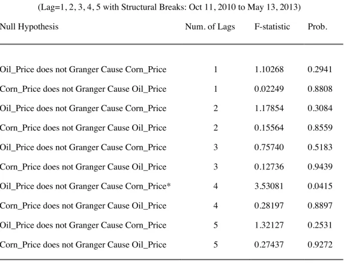
make a large amount of money. In the last period, it may be reasonable to assume that the
causal relationship between oil and corn prices observed in the first period can be resumed to
a certain degree after the financial turbulence. However, the Granger causality test in this
period shows that there is some predictability in corn price, which is the opposite direction to
what we expect. From Figure 1, we can observe that the corn prices decline first and then the
drop in the oil prices follows. The Global Crop Production 2013 states that Corn plunged 40
percent in 2013 as the U.S. is recovering from the prior season when crops were hurt by the
worst drought since the 1930s. The unexpected poor weather condition that prohibits
adequate harvest of corn is obviously uncorrelated with oil market. For the subsequent fall in
the oil prices, despite the low demand for oil that can be partially contributed to the growing
switch away from oil to other fuels like ethanol, other political and economic reasons behind
this price drop such as the turmoil in Iraq and Libya and less need to import oil are not
associated with corn production and crop market. Therefore, we should be really skeptical
this period because it may be merely due to the fact that huge decreases in both prices make
oil and corn much more volatile and the model is deficient in characterizing the whole
dynamics.
Then we proceed with the results of impulse response functions that may provide a more
visual assessment of how oil and corn adjust to one-time shocks both to themselves and to the
other good. In general, Figure 5, 6, 7, 8, 9 all have the responses declining back to the steady
state level. It makes intuitive sense because the VAR model includes only stationary time
series. Therefore, the entire system of equations is stable. Under the full dataset, we can see
that both oil and corn respond to their own exogenous impulses significantly and positively.
These impacts vanish quickly by the second day without any statistically significant
oscillations in later horizons. However, there are no or minor significant adjustments across
commodities, corresponding to the fact that we do not detect any significant unidirectional
causality in the price levels from Granger causality test. Additionally, as we have explained
earlier, the first sub-period has the most stable economic environment while the second and
third ones are largely disturbed. Thus, all the four responses in the first sub-period have the
smallest variance to the exogenous shocks. The forth sub-period is on its way back to
equilibrium while we cannot find the expected causality from corn to oil that should mimic
what found in the first sub-period. Thus, the results are relatively different among different
regimes and we should analyze each regime separately.
In the first sub-period, the percentage change of corn prices responds significantly and
positively to shocks in oil prices although the initial impact quickly mitigates after one day.
However, it is noticeable that a shock in corn prices has an insignificantly minor impact on
the time. Therefore, the corn’s contributions to the volatilities or the size of changes in oil
prices are very limited while the oil’s effect on the volatilities of corn prices is significant. In
the second sub-period, we find that oil prices start to respond to its own shocks in a
significantly oscillating way and the time needed to resume back to the steady state level is
prolonged. Continuing to the third sub-period, we can observe that the time for oil to resume
back to its steady state level is even longer due to higher and more oscillations. However, in
both regimes, even if corn also has a longer response time, it still does not have any
significant oscillations above and below the zero after the initial sharp response to its own
shocks. Moreover, regarding the impulse responses across oil and corn, the significance lies
differently through the process. In the second regime, from Figure 7 b), the percentage price
change of oil does not have a significant initial response to the price shocks of corn.
However, when t=4, a significant oscillation in the response appears. In the third regime,
from Figure 8 c), the initial response of the percentage change of corn prices to oil price
shocks is significant while no significant oscillations can be found later. Due to the highly
volatile economic markets and the rapidly changing investment tastes during these two
periods, any significance in the responses across commodities are supposed to be spurious
and should not be considered meaningful and informative to a large degree. In the forth
post-crisis sub-period, we find inconsistency between our expectation of well-defined
unidirectional causality from corn to oil and the reality of high volatilities, nonexistent
arbitrage and even reversed causality. If we compare Figure 6 and Figure 9 together, we may
find that the underlying mechanism or process for oil to respond to its own shocks is
relatively different. In Figure 6, oil directly and quickly resumes back to its steady state level
after one time horizon. However, in Figure 9, despite the same positively and significantly
initial response, the percentage change of oil prices suffers from more oscillations and spends
inconsistency is partially attributed to the higher volatilities in oil prices and the inelastic
changing economic markets after financial crisis.
Due to the fact of nonexistent arbitrage in the financial market and seemingly spurious
causality between oil and corn at the price levels, we further perform the second moment
causality test in volatilities of oil and corn. As a result, we can see that the change in log likelihood for e!"#$ is highly significant compared to the critical value 𝜒!,!!.!" while the
change in log likelihood for d!"# is not. Therefore, returns of oil at period 𝑡−1 do
statistically significantly help predict the volatility of corn at period 𝑡 while the other way
around is not. In other words, knowing the returns, or the price changes of oil in current
period can help us forecast the uncertainty of oil price in the next period. Moreover, after
controlling for the returns of ethanol and the returns of wheat, we conduct the causality test
again and the estimated coefficients, whose significance represents the causal direction,
correspond to our results in the previous uncontrolled test. In fact, the coefficient estimate of
e!"#$, which represents the second moment causality from the returns of oil to the volatilities
of corn, becomes more significant.
VII. Conclusions
This paper focuses on the better estimation of the correlation between oil and corn with
Realized Beta GARCH model, the first moment Granger Causality test on the prices of oil
and corn, and the second moment causality test on the volatilities and returns of oil and corn
under structural changes. The U.S. biofuel policies, automobile engine technology, and
underlying financial market changes give rise to a complex relationship between oil, ethanol
their prices can move either together or apart. The correlation between oil and corn can be
strengthened, mitigated or fluctuated in the past decade and the causalities of prices,
volatilities and returns between these two commodities can go either direction or even be
insignificant. Based on my results and findings, the correlation between oil and corn prices nearly doubled between 2008 and 2010, corresponding to the trend of increasing investment and financialization of agricultural commodities in the financial market described in Tang and Xiong’s paper (2012). The decrease in the correlation after 2010 may be attributed to the unsynchronized changes in oil and corn prices. Even if both prices dramatically decline, the drop in corn prices precedes the drop in oil prices due to the unexpected exogenous shocks in agricultural production before changes in oil imports.
Conforming to Merkusheva and Rapsomanikis’ conclusion (2012) that oil prices are shown to be the driven forces in the long-run grains prices, we also found that oil prices can Granger cause corn prices before April 2008, which means that current oil prices play a significant role in determining the future corn prices. However, the causality in later years has shown to be insignificant or even weakly reversed. The results from impulse response analysis largely
agree to our causality tests and help draw a limited insight and explanation to certain
confusing phenomena in the forth sub-period. However, there are a number of further
problems that render the interpretation of impulse responses difficult since I only use the
percentage change in the oil and corn prices in the VAR model for simplicity and for
stationarity. The major limitation is the incompleteness or the low-dimension of our model.
In real economic systems, the intertwining relationships between markets, consumers, and
commodities are too complicated to be fully captured. Therefore, we usually have a
simplified yet neater model for computational and interpretation efficiency. However, if
important variables are omitted from the model, we may have major distortions in the
interpretations. Further improvement on the VAR model leaves to future research and
exploration on the first moment causality of oil and corn prices.
However, the bivariate Granger causality model used for the first moment causality test is limited due to its simplicity and thus cannot sufficiently capture the gradual changes in the volatilities and underlying relationship between oil and corn. Therefore, we also conducted the second moment causality test in volatilities and returns of oil and corn. It is much more
sensible, comprehensive and intuitive because the price variables are more likely to follow
the unit root random walks that prohibit people from observing significant predictive power
and from taking advantage of any meaningful relationships among the financial assets, like
oil and corn. Before and after controlling for other stationary variables such as the returns of
wheat and of ethanol, we found that only the coefficient that represents the causality from the
returns of oil to the volatilities of corn is significant.
In conclusion, my empirical research on the evolving relationship between oil and corn here
revealed some interesting and informative features of the correlation and causality between
oil and corn both on the price levels and volatilities. Since 1990s, the U.S. government has
implemented several biofuel policies and a variety of subsidies as a way to reduce
dependence on oil as the energy source and to increase the nation’ overall sustainability.
Based on our findings, during the prior crisis period, namely from 2004 to 2008, changes in
the oil prices that may result from biofuel policy implementation and new standard on the
ethanol production and consumption can have a predictive power in the corn prices.
Therefore, even if ethanol production utilizes a considerable share of total corn use and
diverts valuable crop land away from agricultural production, the increase in the food prices
and costs of animal feed that may put more pressure on crop and livestock farmers as well as
from the financial crisis, any changes in the oil prices are shown to only significantly affect
the volatilities rather than the mere values of corn prices. In other words, the range of the
potential changes of corn prices is enlarged, which entails more uncertainties both in the
energy market and in the food market. Therefore, at present, new policies regarding biofuel
promotion should take these increased volatilities and volatility spillovers between oil and
corn into serious consideration. In fact, based on the increased financialization in the
commodity markets, as indicated by Tang and Xiong in 2012, more non-energy agricultural
commodities, at least those frequently traded in the financial market and used in the energy
production, are more closely associated with the energy market. Therefore, the overall
methodologies used in this paper can be generalized to a larger choice of commodities and
even to a multivariate analysis. The special hierarchical structure of the Realized Beta
GARCH model that combines the flexibility of the GARCH modeling framework with
precise incorporation of volatility measures enables it to be applied to a large variety of
assets, commodities and thus multivariate analysis.
However, despite the advances brought by the relative comprehensive correlation and
causation analysis of oil and corn in this paper, it still does not capture all of the dynamics
between these two goods and further in the larger economic environment. On the one hand,
regarding the first moment causality, I only conducted bivariate Granger causality test out of
simplicity consideration, which can be further improved by taking other relevant factors into
account. Additionally, the specific choice of Cholesky decomposition used in the impulse
response functions is used in the previous papers but sensitive to ordering. Other variance
decomposition method, such as Generalized Variance Decomposition (GVD), may be applied
as well to if the results may be of any difference. On the other hand, however, due to the
nonexistent arbitrage in the financial market, we may rather explore further and deeper on the
release and public speeches from the government can affect the causalities of returns and
volatilities between oil and corn. Any significant results from these modifications and
improvement, in combination with this research, can provide policy makers with more practical insight and feasible guidance to mitigate the potential negative or unpredictable
VII. Bibliography
Bai, J. and Perron, P. (2003). "Computation and analysis of multiple structural change models." Journal of Applied Econometrics 18(1): 1-22.
Balcombe, K. and G. Rapsomanikis, 2008. Bayesian Estimation and Selection of Nonlinear Vector Error Correction Models: The Case of the Sugar-Ethanol-Oil Nexus in Brazil. American Journal of Agricultural Economics, 90(3): 658-668.
Choi, I. and Saikkonen, P. (2004). "Testing linearity in cointegrating smooth transition regressions." Econometrics Journal 7: 341-365.
Chow, G.C., Lin, A.L. (1971), “Best linear unbiased interpolation, distribution and
extrapolation of time series by related series,” The review of Economics and Statistics 53, pp. 372-375.
Kwiatkowski, D., Phillips, P.C.B., Schmidt, P., Shin, Y. (1992). "Testing the null hypothesis of stationarity against the alternative of a unit root." Journal of Econometrics 54: 159-178.
Hansen, Peter R, Asger Lunde, and Valeri Voev. 2014. “Realized Beta Garch: A Multivariate
Garch Model with Realized Measures of Volatility.” Journal of Applied Econometrics 29
(April): 774–779.
Hansen, Peter R, and Zhuo Huang. 2016. “Exponential GARCH Modeling With Realized Measures of Volatility.” Journal of Business & Economic Statistics 34 (2) (March 17): 269–287. http://dx.doi.org/10.1080/07350015.2015.1038543.
Granger, C.W.J., 1969. “Investigating causal relations by econometric models and cross
Granger, C.W.J., 1980. “Testing for causality— a personal viewpoint.” Journal of Economic
Dynamics and Control 2, 329–352.
Granger, 1988. "Some recent developments in a concept of causality." Journal of
Econometrics 39, 199–211.
Tang, Ke, and Wei Xiong. 2012. “Index Investment and the Financialization of Commodities.”
Financial Analysts Journal 68 (6).
Thorp, Susan. n.d. “Crude Oil and Agricultural Futures: An Analysis of Correlation Dynamics.” Discipline of Finance, The University of Sydney Business School, University of Sydney, NSW, 2006, Australia.
Tyner, W. E. and Taheripour, F. (2008). "Policy options for integrated energy and agricultural markets." Review of Agricultural Economics 30: 387-396.
Appendix A. Definitions
Table 1: Definitions of Variables in the Dataset
Variables Definitions
𝑥!"#,! Realized returns of oil at time t calculated from the difference between log prices in a trading day
𝑥!"#$,! Realized returns of corn at time t calculated from the difference between log
prices in a trading day
𝑦!"#,!"#!,! Realized correlation between oil and corn at time t ranging from -1 to 1.
𝑝!"#,! Price of oil at time (trading day) t
𝑝!"#$,! Price of corn at time (trading day) t 𝑝!"!!"#$,! Price of ethanol at time (trading day) t
𝑝!!!"#,! Price of wheat at time (trading day) t
𝑟!"#$%&!'",! Monthly Consumer Price Index (CPI) as a proxy 𝜂! Cross-price elasticity between oil and corn
𝑠! Quarterly corn share used in the energy production
𝑥!"!!"#$,! Realized returns of ethanol at time t calculated from the difference between log prices in a trading day
𝑥!!!"#,! Realized returns of wheat at time t calculated from the difference between log prices in a trading day
Appendix B. Summary Statistics
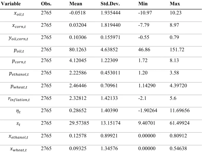
Table 2. Summary Statistics of Variables in the Dataset
Variable Obs. Mean Std.Dev. Min Max
𝑥!"#,! 2765 -0.0518 1.935444 -10.97 10.23
𝑥!"#$,! 2765 0.03204 1.819440 -7.79 8.97
𝑦!"#,!"#$,! 2765 0.10306 0.155971 -0.55 0.79
𝑝!"#,! 2765 80.1263 4.63852 46.86 151.72
𝑝!"#$,! 2765 4.12045 1.22309 1.72 8.13
𝑝!"!!"#$,! 2765 2.22586 0.453011 1.20 3.58
𝑝!!!"#,! 2765 2.46446 0.70961 1.14290 4.39720
𝑟!"#$%&!'",! 2765 2.32812 1.42133 -2.1 5.6
𝜂! 2765 0.28652 1.40390 -1.90264 11.69656
𝑠! 2765 29.57385 13.15174 9.40701 61.49924
𝑥!"!!"#$,! 2765 0.12578 0.89921 0.00000 0.80912
𝑥!!!"#,! 2765 0.09325 1.34576 0.00000 0.54638
Note: This table presents the number of observations (Obs.), average (Mean), standard deviation (Std. Dev.), minimum value (Min) and maximum value (Max) for each variable defined in Table 1. The number of
Appendix C. Preliminary Estimates
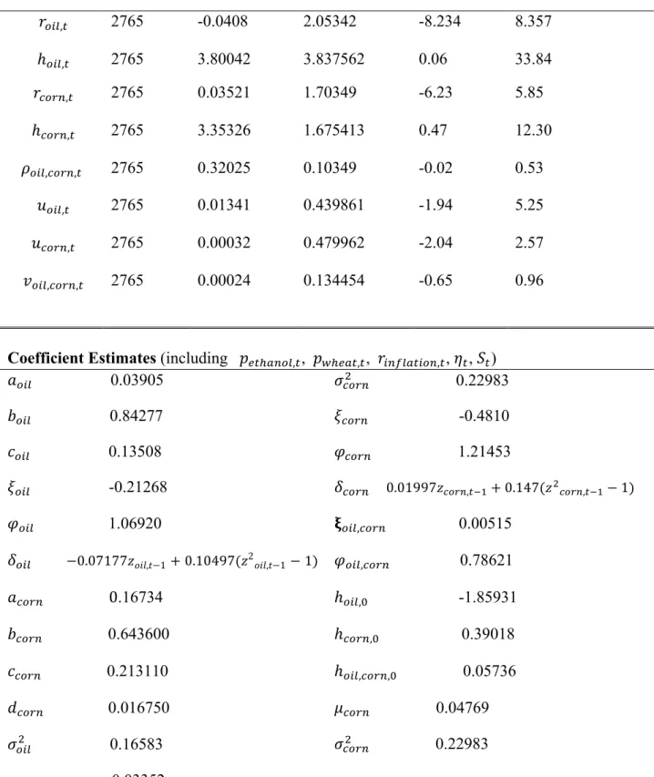
Table 3. Derived Variables and Estimated Coefficients in Realized Beta GARCH Model
Variable Obs. Mean Std.Dev. Min Max
𝑟!"#,! 2765 -0.0408 2.05342 -8.234 8.357
ℎ!"#,! 2765 3.80042 3.837562 0.06 33.84
𝑟!"#$,! 2765 0.03521 1.70349 -6.23 5.85
ℎ!"#$,! 2765 3.35326 1.675413 0.47 12.30
𝜌!"#,!"#$,! 2765 0.32025 0.10349 -0.02 0.53
𝑢!"#,! 2765 0.01341 0.439861 -1.94 5.25
𝑢!"#$,! 2765 0.00032 0.479962 -2.04 2.57
𝑣!"#,!"#$,! 2765 0.00024 0.134454 -0.65 0.96
Coefficient Estimates (including 𝑝!"!!"#$,!, 𝑝!!!!",!, 𝑟!"#$%&!'",!, 𝜂!, 𝑆!)
𝑎!"# 0.03905 𝜎!"#$! 0.22983 𝑏!"# 0.84277 𝜉!"#$ -0.4810
𝑐!"# 0.13508 𝜑!"#$ 1.21453
𝜉!"# -0.21268 𝛿!"#$ 0.01997𝑧!"#$,!!!+0.147(𝑧!!"#$,!!!−1) 𝜑!"# 1.06920 𝛏!"#,!"#$ 0.00515
𝛿!!" −0.07177𝑧𝑜𝑖𝑙,𝑡−1+0.10497(𝑧2𝑜𝑖𝑙,𝑡−1−1) 𝜑!"#,!"#$ 0.78621
𝑎!"#$ 0.16734 ℎ!"#,! -1.85931
𝑏!"#$ 0.643600 ℎ!"#$,! 0.39018 𝑐!"#$ 0.213110 ℎ!"#,!"#$,! 0.05736
𝑑!"#$ 0.016750 𝜇!"#$ 0.04769
𝜎!"#! 0.16583 𝜎
!"#$! 0.22983 𝜇!"# -0.03352
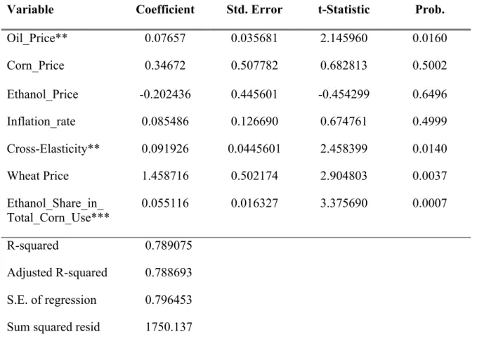
Table 4. OLS Estimates and Structural Breaks from Bai and Perron Procedure
(Dependent Variable: 𝜌!"#,!"#$,!, N:2765)
Variable Coefficient Std. Error t-Statistic Prob.
Oil_Price** Corn_Price
0.07657 0.34672
0.035681 0.507782
2.145960 0.682813
0.0160 0.5002 Ethanol_Price -0.202436 0.445601 -0.454299 0.6496 Inflation_rate 0.085486 0.126690 0.674761 0.4999 Cross-Elasticity** 0.091926 0.0445601 2.458399 0.0140
Wheat Price 1.458716 0.502174 2.904803 0.0037
Ethanol_Share_in_ Total_Corn_Use***
0.055116 0.016327 3.375690 0.0007
R-squared 0.789075 Adjusted R-squared 0.788693 S.E. of regression 0.796453 Sum squared resid 1750.137
Note: 1. * Significant at 10%; ** Significant at 5%; *** Significant at 1%.
2. We use HAC (Heteroskedasticity and Autocorrelation Consistent) covariance estimation in order to allow for serial correlation in the errors.
Breaks F-statistic Scaled F-statistic Weighted F-statistic Critical Value
1* 15.53604 93.21623 93.21623 20.08
2* 28.28419 169.7051 196.1819 17.37
3* 48.56434 291.3860 375.5476 15.58
4* 27.90480 167.4288 241.8683 13.90
5* 32.48390 194.9034 327.7773 11.94
Note: * Significant at 5%
2: Sept 15, 2010, May 13, 2013
3: Apr 01, 2008, Oct 08, 2010, May 13, 2013
4: Nov 1, 2006, Jul 14, 2008, Oct 08, 2010, May 13, 2013
5: Oct 03, 2005, Jun 01, 2007, Jan 22, 2009, Oct 08, 2010
May 13, 2013
Number of Breaks Chosen: 3
Table 5. Bivariate Granger Causality Test Results between Oil and Corn Prices
(Lag=1, 2, 3, 4, 5 without Structural Breaks)
Null Hypothesis Num. of Lags F-statistic Prob.
Oil_Price does not Granger Cause Corn_Price 1 0.51115 0.4747
Corn_Price does not Granger Cause Oil_Price* 1 6.04841 0.0140
Oil_Price does not Granger Cause Corn_Price 2 0.60263 0.5474
Corn_Price does not Granger Cause Oil_Price* 2 3.20563 0.0407
Oil_Price does not Granger Cause Corn_Price 3 0.47950 0.6966
Corn_Price does not Granger Cause Oil_Price 3 2.32010 0.0734
Oil_Price does not Granger Cause Corn_Price 4 1.64446 0.1603
Corn_Price does not Granger Cause Oil_Price 4 1.85162 0.1162
Oil_Price does not Granger Cause Corn_Price 5 1.41912 0.2140
Corn_Price does not Granger Cause Oil_Price 5 1.44856 0.2036
Note: 1. * represents we can reject the null hypothesis at 5% significance level. 2. The F-statistic is defined as !!"(!!"!!!!"!)/!
Table 6. Bivariate Granger Causality Test Results between Oil and Corn Prices
(Lag=1, 2, 3, 4, 5 with Structural Breaks: Jan 05, 2004 to Apr 01, 2008)
Null Hypothesis Num. of Lags F-statistic Prob.
Oil_Price does not Granger Cause Corn_Price** 1 0.9241 0.0091
Corn_Price does not Granger Cause Oil_Price 1 3.27451 0.0708
Oil_Price does not Granger Cause Corn_Price** 2 8.70230 0.0002
Corn_Price does not Granger Cause Oil_Price 2 0.93887 0.0407
Oil_Price does not Granger Cause Corn_Price** 3 6.97756 0.0001
Corn_Price does not Granger Cause Oil_Price 3 0.86169 0.4605
Oil_Price does not Granger Cause Corn_Price** 4 5.20136 0.0004
Corn_Price does not Granger Cause Oil_Price 4 1.09415 0.3580
Oil_Price does not Granger Cause Corn_Price* 5 4.09392 0.0011
Corn_Price does not Granger Cause Oil_Price 5 0.86604 0.5033
Note: 1. * represents we can reject the null hypothesis at 5% significance level. ** represents we can reject the null hypothesis at 1% significance level.
2. The F-statistic is defined as !!"(!!"!!!!"!)/!
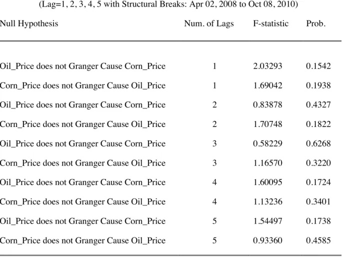
Table 7. Bivariate Granger Causality Test Results between Oil and Corn Prices
(Lag=1, 2, 3, 4, 5 with Structural Breaks: Apr 02, 2008 to Oct 08, 2010)
Null Hypothesis Num. of Lags F-statistic Prob.
Oil_Price does not Granger Cause Corn_Price 1 2.03293 0.1542
Corn_Price does not Granger Cause Oil_Price 1 1.69042 0.1938
Oil_Price does not Granger Cause Corn_Price 2 0.83878 0.4327
Corn_Price does not Granger Cause Oil_Price 2 1.70748 0.1822
Oil_Price does not Granger Cause Corn_Price 3 0.58229 0.6268
Corn_Price does not Granger Cause Oil_Price 3 1.16570 0.3220
Oil_Price does not Granger Cause Corn_Price 4 1.60095 0.1724
Corn_Price does not Granger Cause Oil_Price 4 1.13236 0.3401
Oil_Price does not Granger Cause Corn_Price 5 1.54497 0.1738
Corn_Price does not Granger Cause Oil_Price 5 0.93360 0.4585
Note: 1. * represents we can reject the null hypothesis at 5% significance level. 2. The F-statistic is defined as !!"(!!"!!!!"!)/!
!/(!!(!!!!!)) where 𝑆𝑆𝑅!and 𝑆𝑆𝑅! are the two sums of squared
Table 8. Bivariate Granger Causality Test Results between Oil and Corn Prices
(Lag=1, 2, 3, 4, 5 with Structural Breaks: Oct 11, 2010 to May 13, 2013)
Null Hypothesis Num. of Lags F-statistic Prob.
Oil_Price does not Granger Cause Corn_Price 1 1.10268 0.2941
Corn_Price does not Granger Cause Oil_Price 1 0.02249 0.8808
Oil_Price does not Granger Cause Corn_Price 2 1.17854 0.3084
Corn_Price does not Granger Cause Oil_Price 2 0.15564 0.8559
Oil_Price does not Granger Cause Corn_Price 3 0.75740 0.5183
Corn_Price does not Granger Cause Oil_Price 3 0.12736 0.9439
Oil_Price does not Granger Cause Corn_Price* 4 3.53081 0.0415
Corn_Price does not Granger Cause Oil_Price 4 0.28197 0.8897
Oil_Price does not Granger Cause Corn_Price 5 1.32127 0.2531
Corn_Price does not Granger Cause Oil_Price 5 0.27437 0.9272
Note: 1. * represents we can reject the null hypothesis at 5% significance level. 2. The F-statistic is defined as !!"(!!"!!!!"!)/!