Sharif University of Technology
Scientia IranicaTransactions E: Industrial Engineering http://scientiairanica.sharif.edu
A Malmquist productivity index with the directional
distance function and uncertain data
N. Aghayi
a;, M. Tavana
b;c, and B. Maleki
aa. Department of Mathematics, Ardabil Branch, Islamic Azad University, Ardabil, Iran.
b. Department of Business Systems and Analytics, Lindback Distinguished Chair of Information Systems and Decision Sciences, La Salle University, Philadelphia, PA 19141, USA.
c. Department of Business Information Systems, Faculty of Business Administration and Economics, University of Paderborn, D-33098 Paderborn, Germany.
Received 25 September 2017; received in revised form 13 February 2018; accepted 16 July 2018
KEYWORDS Data envelopment analysis;
Malmquist
productivity index; Interval approach; Directional distance function;
Undesirable outputs.
Abstract. In the present study, by using the directional distance function with undesirable interval outputs, the Malmquist Productivity Index (MPI) and integrated Data Envelopment Analysis (DEA) are employed for evaluating the function of Decision-Making Units (DMUs). The MPI calculation is performed to compare the eciency of the DMUs in distinct time periods. The uncertainty inherent in real-world problems is considered by using the best- and worst-case scenarios, dening an interval for the MPI, and reecting the DMUs' advancement or regress. The optimal solution of the robust model lies in the eciency interval, i.e., it is always equal to or less than the optimal solution in the optimistic case and equal to or greater than the optimal solution in the pessimistic case. This study also presented a case study in the banking industry to demonstrate the applicability and ecacy of the proposed integrated approach.
© 2019 Sharif University of Technology. All rights reserved.
1. Introduction
Building on the ideas of Farrell and twenty years after his pioneering work [1], Charnes et al. [2] developed the DEA technique, which is a non-parametric method for measuring the eciency of a set of Decision-Making Units (DMUs) that use multiple inputs to produce multiple outputs. The model presented by Charnes et al. [2] with a constant return to scale is called the CCR model. In order to devise a new BCC model, some changes were applied to the CCR model by Banker et al. [3]. In DEA models, an inecient
*. Corresponding author.
E-mail addresses: [email protected] (N. Aghayi); [email protected] (M. Tavana); [email protected] (B. Maleki)
doi: 10.24200/sci.2018.5259.1173
DMU could improve its eciency by increasing output levels (produced results) or decreasing input levels (consumed resources). In the real world, however, a DMU may have both desirable and undesirable outputs at the same time. Pittman et al. [4] investigated the use of undesirable outputs to perform an ecient evaluation based on the extended model of Caves et al. [5] so that the eciency of DMUs could be measured in the presence of desirable and undesirable outputs. Further, Ardabili et al. [6] applied undesirable indexes to evaluate DMUs. In addition to comparing the relative performance of a set of DMUs in a specic period, conventional DEA can also be used to calculate the productivity changes of a DMU over time. The Malmquist Productivity Index (MPI) is a model capa-ble of computing the relative performance of a DMU in dierent time periods. Initially termed as a quality productivity index, the MPI was rst introduced in 1953 by Malmquist [7] as ratios of distance functions
for analyzing the consumption of resources in the production. This productivity index was later applied to productivity measurement and analysis. There are several decompositions of the MPI in the literature, with the most popular one proposed by Fare et al. [8]. Now, many researchers consider some degree of data uncertainty in dierent time periods.
In recent years, numerous studies have considered combining data uncertainty in optimized models. How-ever, most of them have relied on complicated non-linear models. Due to the general assumption that the input data are absolutely known, the eects of this issue on exibility and optimality of models have not been considered. Hence, several constraints appear to be violated once the data take values other than their nominal values; the results that have previously ob-tained optimal solution-when nominal data have been investigated-may not remain optimal or even feasible anymore. In the early 1970s, a linear optimization model, which provided a exible solution for input data and could take on any value from an interval, was pro-posed by Soyster [9]. This approach, however, deviated considerably from the nominal problem optimality to ensure the robustness of the solution.
In the current paper, to evaluate the MPI of the DMUs in the best- and the worst-case scenarios, the optimistic and pessimistic models are presented by considering desirable and undesirable interval output data; therefore, the interval has been accomplished for the MPI of the DMUs. In addition, all DMUs are divided into six categories. At the end of intervals, since the maximum coincidence may not be obtained, the considered interval method may not be able to carry out an accurate analysis. Therefore, the purpose of this study is to present an optimized method for computing the MPI of the DMUs. In so doing, the exibility of the obtained solution will no longer be problematic because the accuracy of the solution is guaranteed by the level of conservatism.
1.1. Background
Most DEA papers in recent years have been proposed by researchers to measure the eciency of DMUs. Each of these methods has been developed based on earlier hypotheses. There are generally two approaches in the DEA literature to confronting undesirable outputs. One approach relies on an indirect method presented by Seiford and Zhu [10] following the changes applied to the model suggested by Charnes et al. [2]. Another method is based on the direct approach of Chambers et al. [11], which was developed by Chung et al. [12].
Constrictions of other methods have been some-how eliminated by applying a novel model derived from the model of Shepherd [13]; in addition, e-cient calculations could be carried out in the case of undesirable outputs based on the directional distance
function [14]. Iftikhar et al. [15] used undesirable data in DEA and estimated energy and CO2 emissions.
In order to determine the marginal rates of substi-tution in data envelopment analysis with undesirable outputs, Khoshandam et al. [16] presented a new approach. The MPI facilitates the decomposition of productivity into its two major components, i.e., technological change and technical eciency change. In other words, Malmquist analysis allows separating shifts in the eciency frontier (technological change) from improvements in the eciency associated with the frontier (technical eciency change). These two components are dierent from each other in terms of both basis and analysis and, therefore, require dierent policy measures. The product of technological change and technical eciency change is the total factor productivity change, which is measured by the MPI. A wealth of information can be derived from the MPI. The MPI not only reveals patterns of productivity change and presents a new interpretation along with the managerial implication of each Malmquist com-ponent, but also identies strategic orientations of an organization in past time periods for proper selection in future periods.
Barnabe [17] proposed the application of the Malquist productivity index to power factories. He showed how this index could be used to evaluate the costs of productivity and, also, productivity changes. Sueyoshi et al. [18] measured the eciency of sustain-ability enhancement in China. Sueyoshi and Goto [19] used the MPI for the environmental assessment of petroleum companies. The MPI was also employed by Fuentes and Lillo-Banuls [20] to help perform eciency evaluation of tax oces in Spain from 2004 to 2006. By applying the MPI, Yu et al. [21] carried out an assessment of the eco-eciency performance of the pulp and paper industry in China. Kao [22] measured the MPI for parallel production systems. Maroto and Zoo [23] utilized the Malmquist approach to provide a model for accessibility gains and road transport infrastructure in Spain during the 1995-2005 period. In addition, the overall prot of MPI with interval data and fuzzy was investigated by Emrouznejad et al. [24].
Although there are various methods for optimiza-tion with uncertainty, most of them have problems. In order to confront data uncertainty, a fuzzy approach was adopted by Wanke et al. [25]. He also calculated the eciency of banks. Sorting the genetic algorithm with uncertain data, Mashayekhi and Omrani [26] used a fuzzy approach, too. Aghayi [27] measured cost eciency with fuzzy data in DEA. A framework was presented by Toloo et al. [28], where DEA was used to measure the overall prot eciency with interval data. The eciency of banks with interval data was calculated by Hatami-Marbini et al. [29]. Salehpour
and Aghayi [30] strived to calculate the highest revenue eciency with price uncertainty. In order to nd a solution for minimizing the worst-case performance with uncertain data, Kouvelis and Yu [31] considered a robust optimization model.
For achieving a robust optimal solution, vari-ous approaches were presented by Ben-Tal and Ne-mirovski [32] and El-Ghaoui and Lebret [33]. How-ever, their methods made the robust problem more complex. A robust optimization method, presented by Bertsimas and Sym [34] for linear problems, made the problem more tractable by adjusting the con-servatism degree. Zahedi-Seresht et al. [35] ranked the DMUs based on sensitivity analysis by robust optimization. Youse et al. [36] ranked the sustainable supply chains using network goal programming DEA model and robust fuzzy optimization. For calculating the eciency of vehicle routing operators, Chung-Cheng [37] presented a robust method. In order to measure the technical eciency of potato production in Iran, Mardani and Salarpour [38] employed a robust method. Aghayi et al. [39] investigated the eciency of robust measurement with typical weights, data uncertainty, and various conservatism degrees. To evaluate the eciency measurement of DMUs with undesirable outputs, Aghayi and Maleki [40] applied a robust method.
1.2. Organization
The rest of the paper is organized as follows. Section 2 calculates the MPI of the directional distance function model with undesirable outputs and data uncertainty. In Section 3, by considering interval and robust meth-ods, a model is presented that calculates the MPI based on the directional distance function with undesirable outputs and data uncertainty. Finally, to demonstrate the applicability of the proposed methods, a numerical example is explained in Section 4, which is followed by conclusions in Section 5.
2. Computing the MPI of DMUs with undesirable outputs under data certainty based on the directional distance function model
Here, it is assumed that there are n DMUs with constant inputs, s desirable outputs, and l undesir-able outputs; the desirundesir-able and undesirundesir-able output vectors for DMUj are yj = (y1j; ; ysj) and bj =
(b1j; ; blj), respectively. To evaluate the eciency of
DMUo, the following model was presented by Zanella
et al. [14]:
o = max ;
s.t.:
n
X
j=1
bkjj bko gb; k = 1; ; l; (1a)
n
X
j=1
yrjj yro+ gy; r = 1; ; s; (1b)
n
X
j=1
j= 1;
j 0; j = 1; ; n; (1c)
where g = ( gb; gy) = ( bko; yro). o 0 in all cases;
if
o = 0, then DMUo is ecient; otherwise, DMUo
is inecient. Therefore, the eciency of the evaluated unit can be computed as o= 1+1
o, where 0 < o 1.
For more information on Model (1), refer to Aghayi and Maleki [40]. Model (2) is the dual of Model (1):
o= min
s
X
r=1
yrour+ l
X
k=1
bkodk+ v;
s.t.:
s
X
r=1
gyur+ l
X
k=1
gbdk= 1; (2a)
s
X
r=1
yrjur+ l
X
k=1
bkjdk+v 0; j = 1; ; n; (2b)
ur 0; r = 1; ; s;
dk 0; k = 1; ; l:
Denition 1. In Model (2), if
o = 0, then DMUo
is ecient.
Denition 2. In Model (2), the eciency of DMUo
can be calculated by
o = 1+1
o. Thus, DMUo is
ecient if
o= 1. If o< 1, then DMUo is inecient.
In this section, a model for calculating the MPI is presented. Malmquist analysis relies on the imple-mentation of distance functions. Distance functions based on two distinct time periods as t
o(xt+1; yt+1)
and t+1
o (xt; yt) are dened, where t+1o represents
the distance function associated with the frontier at time t + 1, and (xt+1; yt+1) denotes input and output
vectors at time t + 1. The function t+1 o (xt; yt)
evaluates the input-output combination in period t in relation to technology in period t + 1, whereas the function t
o(xt+1; yt+1) evaluates the observed
input-output combination in period t + 1 in relation to technology in period t. Distance functions for an input-output vector in a specic year in relation to the
frontier in the same year are represented by t o(xt; yt)
and t+1
o (xt+1; yt+1) for years t and t + 1, respectively.
Hence, the directional distance function model with undesirable outputs for the Malmquist index is given as follows:
DMU at time t + 1 and the frontier at time t:
p
o(ypo; bpojp=t; t+1)=min s
X
r=1
yp rour+
l
X
k=1
bpkodk+v;
s.t.:
s
X
r=1
gyur+ l
X
k=1
gbdk= 1;
s
X
r=1
yprjur+ l
X
k=1
bpkjdk+ v 0; j = 1; ; n;
ur 0; r = 1; ; s; dk 0; k = 1; ; l: (3)
DMU at time t and the frontier at time t + 1: p
o(yoq; bqojq; p = t; t + 1; p 6= q) = min s
X
r=1
yq rour+
l
X
k=1
bqkodk+ v
s.t.:
s
X
r=1
gyur+ l
X
k=1
gbdk= 1;
s
X
r=1
yprjur+ l
X
k=1
bpkjdk+ v 0; j = 1; ; n;
ur 0; r = 1; ; s; dk 0; k = 1; ; l: (4)
In Model (3), where the DMU is at time t + 1 and the frontier is at time t, bp and yp represent matrices
corresponding to the desirable and undesirable outputs of the data observed in period p, respectively. Thus, Model (3) is solved for p = t and p = t + 1. Model (4), where the DMU is at time t and the frontier is at time t + 1, is also solved for q, p = t, t + 1, p 6= q.
Denition 3. If the value of the objective function in Models (3) and (4) is zero, then DMUo is ecient.
Denition 4. The eciency score of DMUoin
Mod-els (3) and (4) is calculated by
o = 1+1
o. Hence,
DMUo is ecient if o = 1; if o < 1, then DMUo
is inecient.
When the MPI is to be calculated, there are only two sources of productivity growth, i.e., eciency
change (EFCH) and technical change (TCH), if the production process has constant returns to scale. The geometric mean of these two sources is usually used to calculate the MPI. On the other hand, if the production process exhibits variable returns to scale, the eects of two additional sources of productivity growth, namely pure technical eciency (PTECH) and scale eciency (SECH), are also taken into consideration. As proposed by Ray and Desli [41], calculation of the MPI under variable returns to scale with undesirable outputs in relation to any technology in period t or t + 1 can be performed as follows:
Mo=
s t
v(yt+1o ; bt+1o )
t
v(yto; bto)
t+1v (yot+1; bt+1o )
t+1 v (yot; bto)
s
SEt(yt+1o ; bt+1o )
SEt(yt
o; bto)
SEt+1(yot+1; bt+1o )
SEt+1(yt
o; bto) ; (5)
where t
v measures the productivity growth between
periods t and t + 1 by using the technology of period t as technology, and t+1
v measures the same value
by employing the technology of period t + 1 as the reference technology under Variable Returns to Scale (VRS). Besides, SEt and SEt+1 represent the scale
eciencies when the frontier is in periods t and t + 1, respectively, and are given by:
SEt(yt+1
o ; bt+1o ) = t
c(yt+1o ; bt+1o )
t
v(yot+1; bt+1o );
SEt+1(yt+1
o ; bt+1o ) = t+1
c (yt+1o ; bt+1o )
t+1
v (yt+1o ; bt+1o ); (6)
SEt(yt
o; bto) = t c(yto; bto)
t
v(yot; bto);
SEt+1(yt
o; bto) = t+1 c (yot; bto)
t+1
v (yot; bto); (7)
where t
c and t+1c assess the productivity growth
under constant returns to scale in periods t and t + 1, respectively. The results are interpreted as follows:
1. Mo> 1 shows productivity increase or progress;
2. Mo< 1 reveals productivity decrease;
3. Mo= 1 reects unchanged productivity during the
two periods.
3. Calculating the MPI of DMUs with undesirable outputs with data uncertainty based on the directional distance function model
Here, it is considered that there are n DMUs with constant inputs, s desirable interval outputs, and l
undesirable interval outputs; the desirable and undesir-able output vectors for DMUj are yj = (y1j; ; ysj)
and bj = (b1j; ; blj), respectively, where yj 2
[yL
j; yUj ] and bj 2 [bLj; bUj]. yLj and bLj, respectively,
indicate the lower bound of desirable and undesirable outputs for DMUj. For calculating MPI for DMUo
with data uncertainty, the following models can be used:
DMU at time t + 1 and the frontier at time t: p
o(ypo; bpojp=t; t+1)=min s
X
r=1
yp rour+
l
X
k=1
bp kodk+v
s.t.:
s
X
r=1
gyur+ l
X
k=1
gbdk= 1;
s
X
r=1
yprjur+ l
X
k=1
bp
kjdk+ v 0; j = 1; ; n;
ur 0; r = 1; ; s; dk 0; k = 1; ; l: (8)
DMU at time t and the frontier at time t + 1: p
o(yoq; bqojq; p = t; t + 1; p 6= q ) = min s
X
r=1
yq rour+
l
X
k=1
bq
kodk+ v;
s.t.:
s
X
r=1
gyur+ l
X
k=1
gbdk= 1;
s
X
r=1
yp rjur+
l
X
k=1
bp
kjdk+v 0; j =1; ; n;
ur 0; r = 1; ; s; dk 0; k = 1; ; l: (9)
In the following, two approaches to solving Mod-els (8) and (9) are presented: one is based on interval concepts and the other relies on robust optimization. 3.1. Calculating MPI based on the interval
approach
In Models (8) and (9), due to the changes in input and output parameters over interval, the values of DMUs eciency are included in the interval. The eciency value of the DMUs for the upper and lower bounds can be calculated in the following. To calculate the eciency value of lower bound, the DMU is evaluated in the worst-case scenario (lower bound with its desir-able output and the upper bound with its undesirdesir-able
output) and the other DMUs in the best-case scenario (by exploring the upper bound of desirable outputs and the lower bound of undesirable outputs). Thus, in pessimistic conditions, to measure the eciency of DMU0 based on the directional distance function, the
following models are presented:
DMU at time t + 1 and the frontier at time t:
Lp
o (yLpo ; bUpo jp=t; t+1)=min s
X
r=1
yLp rour+
l
X
k=1
bUpkodk+v;
s.t.:
s
X
r=1
gyur+ l
X
k=1
gbdk= 1;
s
X
r=1
yUprjur+ l
X
k=1
bLpkjdk+ v 0;
j = 1; ; n; j 6= o;
s
X
r=1
yLp rour+
l
X
k=1
bUpkodk+ v 0;
ur 0; r =1; ; s; dk 0; k =1; ; l: (10)
DMU at time t and the frontier at time t + 1: Lp
o (yLqo ; bUqo jq; p = t; t + 1; p 6= q ) = min s
X
r=1
yLq rour+
l
X
k=1
bUqkodk+ v
s.t.:
s
X
r=1
gyur+ l
X
k=1
gbdk= 1;
s
X
r=1
yrjUpur+ l
X
k=1
bLpkjdk+ v 0;
j = 1; ; n; j 6= o;
s
X
r=1
yLq rour+
l
X
k=1
bUqkodk+ v 0;
ur 0; r =1; ; s; dk 0; k =1; ; l: (11)
Denition 5. In Models (10) and (11), DMUois said
to be ecient under pessimistic conditions if LP o = 0.
Denition 6. Eciency measure in the lower bound is given by LP
o = 1+1LP o . If
LP
o = 1, then DMUo is
ecient.
Conclusion 1. The lower bound of the MPI is calculated as follows:
ML=
s Lt
v yt+1o ; bt+1o
Ut
v (yot; bto)
Lt+1
v yot+1; bt+1o
Ut+1 v (yto; bto)
s
SELt yt+1 o ; bt+1o
SEUt(yt
o; bto)
SELt+1 yt+1 o ; bt+1o
SEUt+1(yt
o; bto) : (12)
From an optimistic perspective, when the evaluated DMU is investigated in the best-case scenario, it means that the upper bound is considered in its desirable output and the lower bound is considered in its un-desirable output. In addition, when the other DMUs are investigated in the worst-case scenario, it means that the lower bound is considered in desirable outputs and the upper bound is considered in undesirable outputs. For calculating the optimistic eciency of DMUo according to the directional distance function,
the following models can be used:
DMU at time t + 1 and the frontier at time t: Up
o (yoUp; bLpo jp = t; t + 1) = min s
X
r=1
yUp rour+
l
X
k=1
bLpkodk+ v;
s.t.:
s
X
r=1
gyur+ l
X
k=1
gbdk= 1;
s
X
r=1
yrjLpur+ l
X
k=1
bUpkjdk+ v 0;
j = 1; ; n; j 6= o;
s
X
r=1
yUp rour+
l
X
k=1
bLpkodk+ v 0;
ur 0; r =1; ; s; dk 0; k =1; ; l: (13)
DMU at time t and the frontier at time t + 1: Up
o (yoUq; bLqo jq; p = t; t + 1; p 6= q ) = min s
X
r=1
yUq rour+
l
X
k=1
bLqkodk+ v;
s.t.:
s
X
r=1
gyur+ l
X
k=1
gbdk= 1;
s
X
r=1
yrjLpur+ l
X
k=1
bUpkjdk+ v 0;
j = 1; ; n; j 6= o;
s
X
r=1
yUq rour+
l
X
k=1
bLqkodk+ v 0;
ur 0; r =1; ; s; dk 0; k =1; ; l: (14)
Denition 7. In Models (13) and (14), DMUois said
to be ecient under optimistic conditions if Up o = 0.
Denition 8. Optimistic eciency measures in Mod-els (13) and (14) are given by Up
o = 1+1Up o . If
Up o = 1,
then DMUo is ecient.
Conclusion 2. The upper bound of the MPI is calculated as follows:
MU=
s Ut
v yot+1; bt+1o
Lt
v (yto; bto)
Ut+1
v yot+1; bt+1o
Lt+1 v (yto; bto)
s
SEUt yt+1 o ; bt+1o
SELt(yt
o; bto)
SEUt+1 yt+1 o ; bt+1o
SELt+1(yt
o; bto) : (15)
Theorem 1. Prove ML MU.
Proof. For indicating Up
o oLp, we must prove that,
in Models (10) and (11), the values of objective function are smaller than those for Models (13) and (14), that is to say, Lp
o Upo 0. For optimistic and pessimistic
models, the values of objective function are considered as follows:
Lp
o =
s
X
r=1
uryLpro + l
X
k=1
dkbUpko + v;
Up
o =
s
X
r=1
uryUpro + l
X
k=1
dkbLpko + v: (16)
Now, obtaining the result of LP
o oUP, we can write:
Lp
o Upo = s
X
r=1
ur(yUpro yroLp)
+
l
X
k=1
Considering the fact that ur, dk 0, yroUp yroLp, and
bUpko bLpko, Eq. (17) will be a positive value. Therefore, Up
o Lpo ; it is also obvious that Lpo Upo . Now, let
the lower and upper bounds be given by:
ML=
s Lt
v yot+1; bt+1o
Ut
v (yto; bto)
Lt+1
v yot+1; bt+1o
Ut+1 v (yot; bto)
s
SELt yt+1 o ; bt+1o
SEUt(yt
o; bto)
SELt+1 yt+1 o ; bt+1o
SEUt+1(yt o; bto) ;
MU=
s Ut
v yot+1; bt+1o
Lt
v (yto; bto)
Ut+1
v yt+1o ; bt+1o
Lt+1 v (yot; bto)
s
SEUt yt+1 o ; bt+1o
SELt(yt
o; bto)
SEUt+1 yt+1 o ; bt+1o
SELt+1(yt
o; bto) : (18)
Since Lp
o Upo , it is obvious that ML MU.
Conclusion 3. If MU
o and MoL are the upper and
lower bounds of the MPI, respectively, as obtained by the directional distance function, then Mo 2
[ML o; MoU].
By considering that the MPI of each DMU lies at an interval, the DMUs can be divided into six categories:
a. DMUs with constant productivity, i.e., Eo =
fDMUj: MjU = MjL = 1g;
b. All DMUs with increasing productivity and progress in the pessimistic case, i.e., E++ = fDMUj : 1 <
ML
j MjUg;
c. All DMUs with decreasing productivity and regress in the optimistic case, i.e., E = fDMUj : MjL
MU j < 1g;
d. All DMUs with increasing productivity in the op-timistic case and unchanged productivity in the pessimistic case, i.e., E+ = fDMU
j : MjL =
1; MU j > 1g;
e. All DMUs with decreasing productivity in the pes-simistic case and unchanged productivity in the optimistic case, i.e., E = fDMUj : MjL <
1; MU j = 1g;
f. All DMUs with increasing productivity in the op-timistic case and decreasing productivity in the pessimistic case, i.e., E = fDMUj : MjL < 1 <
MU j g.
3.2. Calculating the MPI based on the robust approach
There are n DMUs, DMUj (j = 1; ; n), with
de-sirable and undede-sirable interval outputs. jJjyj and jJb jj
are the number of desirable and undesirable outputs
in the jth constraint, respectively. The role of jjyj and jb
jj parameters (yj 2 [0; jJjyj] and jb 2 [0; jJjbj])
is adapting the robustness of the considered method in the conservation level of the solution. Here, the purpose is to ensure that the obtained solution will remain exible when yj and b
j are changed by (jy
[jy])(ytjUp yLptj ) and (b
j [jb])(bUptj bLptj ). In other
words, the behavior of data related to the desirable and undesirable outputs highly depends on this assumption that changes in a subset of coecients adversely aect the solution. Therefore, we can be ensured that the optimal robust solution remains feasible. For eciency assessment, the following robust models are presented: DMU at time t + 1 and the frontier at time t:
Rp
o (yUpo ; bLpo jp = t; t + 1) = min s
X
r=1
yUp rour+
l
X
k=1
dkbLpko + v
+ max
Coy
( X
r2SY o
ur yUpro yroLp
+ (y
o [oy]) uyto yroUp yLpro
)
+ max
Cb o
( X
k2Sb o
dk
bUpko bLpko
+ b o [ob]
db
to
bUpto bLpto);
s.t.:
l
X
k=1
gbdk+ s
X
r=1
gyur= 1; (19a)
s
X
r=1
yLprjur l
X
k=1
bUpkjdk+max cy
j
( X
r2SY j
ur
yUprj yrjLp
+ (y
o [yo]) uytj
ytjUp ytjLp)
+ max
cb j
( l X
k2Sb j
dk
bUpkj bLpkj
+ b j [jb]
db
tj
j = 1; ; n; j 6= o; (19b)
s
X
r=1
yUp rour+
l
X
k=1
dkbLpko + v
+ max
Cy o
( X
r2SY o
ur yUpro yLpro
+ (y
o [oy]) uyto yroUp yroLp
)
+ max
Cb o
( X
k2Sb o
dk
bUpko bLpko
+ b o [ob]
db
to
bUpto bLpto) 0; (19c)
ur 0; r =1; ; s; dk 0; k =1; ; l:
DMU at time t and the frontier at time t + 1: Rp
o (yoUq; bLqo jq; p = t; t + 1; p 6= q ) = min s
X
r=1
yUq rour+
l
X
k=1
dkbLqko + v
+ max
Cy o
( X
r2SY o
ur yroUq yroLq
+ (y
o [oy]) uyto yUqro yLqro
)
+ max
Cb o
( X
k2Sb o
dk
bUq
ko bLqko
+ b o [ob]
db
to
bUqto bLqto);
s.t.:
l
X
k=1
gbdk+ s
X
r=1
gyur= 1; (20a)
s
X
r=1
yLprjur l
X
k=1
bUpkjdk
+ max
cyj
( X
r2SY j
ur
yUprj yLprj
+ (y
o [yo]) uytj
ytjUp ytjLp)
+ max
cb j
( l X
k2Sb j
dk
bUpkj bLpkj
+ b j [jb]
db
tj
bUptj bLptj ) v 0;
j = 1; ; n; j 6= o; (20b)
s
X
r=1
yUq rour+
l
X
k=1
dkbLqko + v
+ max
Cy o
( X
r2SY o
ur yUqro yLqro
+ (y
o [oy])uyto yUqro yLqro
)
+ max
Cb o
( X
k2Sb o
dk
bUqko bLqko
+ b o [bo]
db
to
bUqto bLqto) 0; (20c)
ur 0; r =1; ; s; dk 0; k =1; ; l:
where: Cy
j = fSjy[ ftyjgjSjy Jjy;Sjy
= [jy]; tyj 2 (tyj Sjy)g; j = 1; ; n;
Cb
j = fSjb[ ftbjgjSjb Jjb;Sjb
= [b
j]; tbj 2 (tbj Sjb)g; j = 1; ; n; (21)
where tj and Sj are related to the data with and
without perturbation, respectively. Now, if it is assumed that b
j = 0 and yj = 0, then Models (19)
and (20) are equivalent to Models (13) and (14), respectively; likewise, if b
j = jJjbj and jy = jJjyj, then
Models (19) and (20) are equivalent to Models (10) and (11), respectively. After all, since Models (20) and (21) are nonlinear and dicult to solve, they can be transformed into the following linear models by applying the approach proposed by Bertsimas and Sim [34], where zj denotes total data perturbations.
jy= max
cy j
( X
r2SY j
ur
yrjUp yrjLp
+ (y
o [oy]) uytj
ytjUp ytjLp);
j = 1; ; n;
b j = max
cb j
( l X
k2Sb j
dk
bUpkj bLpkj
+ b j [jb]
db
tj
bUptj bLptj );
j = 1; ; n: (22) In order to obtain a linear form of Model (19), Models (23) and (24) respectively correspond to desir-able and undesirdesir-able outputs in Constraint (19a):
jy= max
cy j
( X
r2SY j
ur
yrjUp yrjLp
+ (y
o [oy]) uytj
ytjUp ytjLp);
s.t.: X
j2jJy jj
zjy Y
j ; (23a)
0 zj 1: (23b)
b j = max
cb j
( l X
k2Sb j
dk
bUpkj bLpkj
+ b j [jb]
db
tj
bUptj bLptj )
s.t.: X
j2jJb jj
zb
j bj; (24a)
0 zj 1; (24b)
where zj shows the sum total of data uctuations.
Now, taking prj and qkj as dual variables of
Con-straints (23a) and (24a), respectively, Constraint (19b) can be rewritten as follows:
s
X
r=1
uryrjLp+ zjyjy+ s
X
r=1
prj l
X
k=1
dkbUpkj + zjbjb
+Xl
k=1
qkj v 0; j = 1; ; n; j 6= o;
zjy+ prj ur
yUprj yLprj; r = 1; ; s; j = 1; ; n; zb
j+ qkj dk
bUpkj bLpkj; k = 1; ; l; j = 1; ; n; ur 0; r = 1; ; s;
dk 0; k = 1; ; l;
zjy 0; zb
j 0; j = 1; ; n;
prj 0; j = 1; ; n; r = 1; ; s;
qkj 0; j =1; ; n; k =1; ; l: (25)
By applying the strong duality theorem and, also, con-sidering the fact that Models (23) and (24) are feasible and bounded, it can be concluded that their corre-sponding dual problem is feasible and bounded, too.
Model (19) can be converted into a linear form so that Model (26) can be obtained as follows:
DMU at time t + 1 and the frontier at time t: Rp
o (yUpo ; bLpo jp = t; t + 1) = min s
X
r=1
uryroUp
+ zy ooy+
s
X
r=1
pro+ l
X
k=1
dkbLpko + zobob
+Xl
k=1
qko+ v; (26)
s.t.:
s
X
r=1
urgy+ l
X
k=1
dkgb= 1; (26a)
s
X
r=1
uryrjLp+ zjyjy+ s
X
r=1
prj l
X
k=1
dkbUpkj + zjbjb
+
l
X
k=1
j = 1; ; n; j 6= o; (26b)
s
X
r=1
uryUpro + zyooy+ s
X
r=1
pro+ l
X
k=1
dkbLpko + zobbo
+Xl
k=1
qko+ v 0; (26c)
zyj + prj ur(yUprj yLprj);
r = 1; ; s; j = 1; ; n; (26d) zb
j+ qkj dk(bUpkj bLpkj);
k = 1; ; l; j = 1; ; n; (26e) R
o 1; (26f)
zyj 0; zb
j 0; j = 1; ; n;
prj 0; qkj 0; r = 1; ; s;
k = 1; ; l; j = 1; ; n; ur 0; dk 0; r = 1; ; s;
k = 1; ; l:
DMU at time t and the frontier at time t + 1:
yUq
o ; bLqo jq; p = t; t + 1; p 6= q ) = min s
X
r=1
uryUqro
+ zy ooy+
s
X
r=1
pro+ l
X
k=1
dkbLqko + zobob
+
l
X
k=1
qko+ v;
(27) s.t.:
s
X
r=1
urgy+ l
X
k=1
dkgb= 1; (27a)
s
X
r=1
uryLprj + zyjjy+ s
X
r=1
prj l
X
k=1
dkbUpkj + zbjjb
+Xl
k=1
qkj v 0;
j = 1; ; n; j 6= o; (27b)
s
X
r=1
uryUqro + zyooy+ s
X
r=1
pro+ l
X
k=1
dkbLqko + zboob
+Xl
k=1
qko+ v 0;
(27c) zyj + prj ur(yUprj yrjLp);
r = 1; ; s; j = 1; ; n; (27d) zb
j+ qkj dk(bUpkj bLpkj);
k = 1; ; l; j = 1; ; n; (27e) R
o 1; (27f)
zyj 0; zb
j 0; j = 1; ; n;
prj 0; qkj 0; r = 1; ; s;
k = 1; ; l; j = 1; ; n; ur 0; dk 0; r = 1; ; s;
k = 1; ; l:
Note that all theorems with regard to Model (26) are proven; similarly, all of them can also be proven for Model (27).
Theorem 2. Proving Model (26) is always feasible. Proof. We consider zj = 0 (j = 1; ; n), jy =
b
j = 0 (j = 1; ; n), and prj = qkj = 0 (8 r; k; j =
1; ; n). Since 2 R, we can suppose that = 1. In addition, it is considered here that dk = 08 k,
ur = y1ro8 j = o, and ur = 08 j 6= o; it must be
mentioned that gy = yUpro is in Constraint (26a). By
substituting these assumptions in Constraint (26a), we have:
s
X
r=1
1
yUpro yro+ 0 = 1; (28)
which always holds.
By substituting the above equation into con-straint (26b), we have:
0 v 0; j = 1; ; n j 6= o; (29) which always holds for = 1. The obtained solution satises Constraint (26c). Since y
j = jb = 0 (j =
1; ; n), we can add to Constraints (26d) and (26e) the following:
yrjUp yLprj = 0; 8 r; j = 1; ; n;
bUpkj bLpkj = 0; 8 k; j = 1; ; n: (30) Consequently, Constraints (26c) and (26d) hold. Since the value of the objective function in the obtained solu-tion equals 1, Constraint (26f) holds, thus completing the proof.
Denition 9. In Models (26) and (27), DMUo is
ecient if Rp o = 1.
Conclusion 4. The eciency scores of Models (26) and (27) are given by Rp
o = 1+1Rp o .
Conclusion 5. Calculation of the MPI using the robust approach is as follows:
MR=
s Rt
v yot+1; bt+1o
Rt
v (yot; bto)
Rt+1
v yt+1o ; bt+1o
Rt+1 v (yto; bto)
s
SERt yt+1 o ; bt+1o
SERt(yt
o; bto)
SERt+1 yt+1 o ; bt+1o
SERt+1(yt
o; bto) : (31)
Theorem 3. Prove MR MU.
Proof. The values of objective function for Mod-els (26) and (13) are given by the following two relations:
s
X
r=1
uryroU + zoyoy+ s
X
r=1
pro+ l
X
k=1
dkbLko+ zobob
+Xl
k=1
qko+ v; (32)
and:
s
X
r=1
yU rour+
l
X
k=1
bL
kodk+ v: (33)
Since pr, qk, zyo, zob, oy, bo are positive, Eq. (32) is
greater than Eq. (33). Thus, eciency scores Rp o
in Models (26) and (27) are smaller than eciency scores Up
o in Models (13) and (14). Hence, it becomes
obvious that MR MU.
Algorithm 1 summarizes computing the MPI of the DMUs with undesirable outputs and data uncer-tainty according to the directional distance function.
4. Numerical example
In order to demonstrate the applicability of the con-sidered methods, a simple example including 5 DMUs, each of which produces one desirable and one undesir-able interval output, is expressed in Subsection 4.1. In addition, a case study of data related to the National Bank branches in Ardabil, Iran is investigated in Subsection 4.2. Then, in Subsection 4.3, the results of Aghayi and Maleki [40] and those obtained from the proposed models will be compared.
4.1. Simple example
Here, 5 DMUs are considered, each of which with two interval outputs-one desirable, one undesirable-in time periods t and t + 1, as shown in Tables 1 and 2.
The results of solving Models (3), (4), (10), (11), (13), (14), (26), and (27) are represented in Table 3.
According to Table 3, all DMUs fall into the sixth category; for all cases, the productivity rise in the op-timistic scenario is greater than that in the pessimistic scenario. Having eciency scores smaller than one under both the optimistic and pessimistic scenarios, only DMU2 belongs to the third category. In the
optimistic scenario, the DMUs can be ranked in terms of productivity progress as DMU3> DMU1> DMU4,
DMU5 > DMU2. Under the pessimistic scenario,
the DMUs are ranked based on productivity regress as DMU1 > DMU3 > DMU2 > DMU4 > DMU5.
It is worth mentioning that the order of productivity rise may be dierent from that of productivity decline. Since one desirable output and one undesirable output are dealt with in this simple numerical example, y
o = 1
and b
o= 1 when the robust approach is implemented.
In order to calculate Rpj , the average value of eciency is divided into two decimal places for each . In
Table 1. Data related to the desirable outputs in time periods t and t + 1.
DMU ylt
j yjlt+1 yjut yjut+1
1 5 10 9 13
2 5 10 9 11
3 15 20 21 22
4 10 15 20 20
5 30 35 31 37
Table 2. Data pertaining to undesirable outputs in time periods t and t + 1.
DMU blt
j blt+1j butj but+1j
1 5 10 8 15
2 15 20 20 25
3 20 25 22 30
4 40 45 42 50
5 25 30 27 35
Table 3. Results of solving Models (3), (4), (10), (11), (13), (14), (26), and (27).
DMU Mj Mj Mj MjR
1 0.98 0.66 1.32 1 2 1.07 0.81 0.95 0.94 3 1.00 0.75 1.47 0.92 4 1.09 0.85 1.25 0.94
5 1 0.90 1.25 1
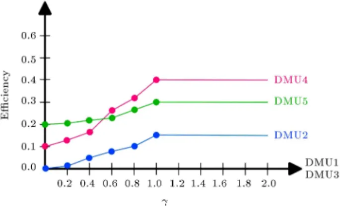
Figure 1. Eciency values of the DMUs for various values.
addition, this example considered 2 [0; 2] with a step length of 0.2. In this regard, it is assumed that there are two random parameters: for simplication, = y
o+ob. Based on the comparison of the results for
MR
j in Table 3, it is observed that there is no change in
productivity at time t + 1 as compared to productivity at time t, because MR
1; M5R = 1. Furthermore,
MR
2 ; M3R; M4R< 1 implies productivity regress.
Considering the two random parameters simpli-ed in the following form: = y
o + bo, Figure 1
shows eciency changes for dierent values of . As observed in Figure 1, the maximum coincidence occurs for 2 [1; 2], that is to say, data uctuations do not aect eciency when the value of is equal to or greater than 1.
4.2. Case study
Nowadays, the signicant role of nancial institutions is no secret to anyone. In most countries, banks play an integral role in this regard; they aect the economic performance of countries through mobilizing resources, providing means of payment, granting facilities, and creating interactions between investment and saving. Since the most important mission of the banking system is the collection and optimal allocation of public funds to productive economic activities, the volume of granted facilities in return for a specic level of used inputs and deposits remains one of the primary criteria for evaluating the proper performance of each bank. The application of the MPI proves to be one of the main methods of evaluating the performance of banks. In fact, higher eciency and productivity of the banking industry in any country is synonymous with lower banking costs, higher interest rates, and superior service quality, leading ultimately to a decrease in investment costs. In order to show that the proposed methods herein are applicable to real-world environ-ments, where interval data and undesirable outputs are dealt with, the eciency of 30 branches of the National Bank in Ardabil Province, Iran over a 4-year period from 2011 to 2014 was evaluated.
With this end in view, each branch of National Bank was considered a DMU with constant inputs, such as the terms and values of deposits required for getting loans and the rate of interest for each loan, which are all xed and identical in all branches of the National Bank of Iran. This study adopts an intermediate approach, whereby nancial institutions such as banks are merely nancial intermediaries and assume two major roles of receiving and distributing resources in the economy. By virtue of this approach, we will dene an indicator for desirable outputs, which are revenue per branch. Moreover, non-performing loans and the amount of four main types of deposits-i.e., interest{free deposits, short-term investment deposits, long-term investment deposits, and current deposits{are dened as indicators of undesirable outputs. Since we always treat inputs as undesirable outputs, the amount of deposits is taken as an undesirable index. In order to evaluate the eciency of these branches, Models (10), (11), (13), and (14) are rst employed for eciency measurement under optimistic and pessimistic scenarios and, then, the branches are divided into the six categories mentioned above. Then, for nding a deterministic solution, the proposed robust model is used. According to Table 4, the last column includes values of eciency obtained by executing Model (13). For calculating this column, the average values achieved through solving Models (26) and (27) for a step length of 0.2 have been used. In addition, because there are one desir-able and two undesirdesir-able outputs in this evaluation, 2 [0; 3]. In comparison with other similar models, the advantage of using the robust model is that its results are of high validity since it is calculated in the worst-case scenario. DMU2, DMU3, and DMU21
exhibit progress because MR
2 , M3R, M21R > 1; M4R,
MR
5, M22R, M23R, M24R = 1; therefore, nothing can
be said about these DMUs; the other DMUs have regress. It can be seen that ML
j MjU and MjR
MU
j , reecting the fact that the obtained results are
completely consistent with the proven theorems herein. The results of calculating the MPI of the considered National Bank branches of Iran are demonstrated in Figure 2.
Figure 2. Comparison of the results by calculating the MPI of the National Bank of Iran branches.
Table 4. Results of the MPI of National Bank of Iran branches.
DMU Mj Mj Justication MjR
1 0.563065 1.14586 E 0.910306 2 0.578326 1.149271 E 1.03923 3 0.671972 1.082658 E 1.024695
4 0.892928 1.314586 E 1
5 0.978419 1 E- 1
6 0.694989 0.849843 E - - 0.737387 7 0.756402 0.889302 E - - 0.843447 8 0.59453 0.8721 E - - 0.755794
9 0.687906 1.016441 E 1
10 0.562258 1.020162 E 0.872228 11 0.554886 0.989638 E - - 0.843412 12 0.601147 0.897519 E - - 0.769528 13 0.615545 0.916612 E - - 0.774725 14 0.726207 1.40005 E 0.943396 15 0.864611 1.068994 E 0.980392 16 0.798679 0.857059 E - - 0.620269 17 0.720033 1.216943 E 0.798111 18 0.732865 1.070131 E 0.882346 19 0.566529 1.023449 E 0.966736 20 0.59957 0.903914 E - - 0.84112 21 0.893314 1.314533 E 1.075905
22 0.707107 1.112718 E 1
23 0.707107 1.211172 E 1
24 0.731272 1.058372 E 1
25 0.508698 1.112751 E 0.884956 26 0.525051 0.948891 E - - 0.74511 27 0.638628 0.95121 E - - 0.755882 28 0.601131 0.840623 E - - 0.750766
29 0.704135 1.012594 E 1
30 0.554469 0.917087 E - - 0.76716
4.3. Comparison with the paper authored by Aghayi and Maleki [40]
In this section, the results obtained by applying the proposed robust Malmquist model{which is based on the Directional Distance Function (DDF) and is also eective in the presence of undesirable outputs{to 30 branches of the National Bank of Iran across Ardabil, Iran, are compared with those obtained from the DDF-based robust model proposed by Aghayi and Maleki [40]. The results of executing the DDF-based robust model for a step length of 0.2 are given in Table 5. Considering the fact that, in this evaluation, we deal with one desirable and two undesirable outputs, 2 [0; 3]. These results have been produced by analyzing data from 2011 to 2014. Datasets related to 2011 and 2014 have been taken as the lower and
Table 5. Results of the comparison between the proposed method and Aghayi and Maleki's method [40].
DMU R
j MjR
1 1 0.910306
2 1 1.03923
3 1 1.024695
4 1 1
5 1 1
6 1 0.737387
7 0.84 0.843447
8 1 0.755794
9 1 1
10 1 0.872228
11 1 0.843412
12 1 0.769528
13 1 0.774725
14 1 0.943396
15 1 0.980392
16 0.81 0.620269
17 0.93 0.798111
18 0.59 0.882346
19 1 0.966736
20 1 0.84112
21 0.92 1.075905
22 1 1
23 1 1
24 0.99 1
25 1 0.884956
26 1 0.74511
27 1 0.755882
28 1 0.750766
29 1 1
30 1 0.76716
upper bounds, respectively. As shown in Table 5, the number of ecient units according to the DDF-based robust model proposed by Aghayi and Maleki [40] is too high, stressing the need for ranking ecient DMUs. Yet, the results of the DDF-based robust Malmquist model demonstrate that over a four-year period from 2011 to 2014, only 3 units exhibited progress, 7 units did not have progress, and other units showed regress. Moreover, Figure 3 compares the results of the
DDF-Figure 3. Comparison of the results in this paper with those in Aghayi and Maleki's method [2].
based robust Malmquist model with those obtained by the DDF-based robust model proposed by Aghayi and Maleki [40].
5. Conclusion
Data uncertainty is one of the main concerns of indus-trial, economic, and manufacturing planners. Thus, it is important to achieve robust optimal solutions to these problems. In the current paper, the MPI and the DEA technique were used to investigate the eciency status and productivity changes of the branches of the National Bank of Iran across Ardabil, Iran, during four consecutive years. Initially, the present paper consid-ered the interval-data of Malmquist model based on the directional distance function with undesirable outputs; by increasing the desirable outputs and decreasing the undesirable outputs, it simultaneously evaluated the eciency values. Then, it was shown that the eciency value was not certain and, instead, depended on an interval. Next, in order to assess the DMUs, they were divided into six categories. After that, the DDF-based robust Malmquist model was presented in the presence of undesirable outputs, without increasing the problem complexity. The proposed model aimed to minimize the maximum value of the objective function with the optimization of the worst-case scenario. Moreover, by dening a conservatism level, the feasibility of optimal solution was guaranteed. The biggest advantage of the considered robust model is that since the conservatism degree is adjustable, the proposed method performs conservatively and provides a deterministic solution. Designing a robust model for calculating the MPI of the DUMs with undesirable outputs along with fuzzy and negative data is suggested for future researches.
Acknowledgement
The research was carried out during a sabbatical stay by Nazila Aghayi at the Universite Catholique de Louvain. Financial support by Ardabil branch, Islamic Azad University, Ardabil, Iran is gratefully acknowledged.
References
1. Farrell, M.J. \The measurement of productive ef-ciency", Journal of the Royal Statistical Society, 120(3), pp. 253-281 (1957).
2. Charnes, A., Cooper, W.W., and Rhodes, E. \Measur-ing the eciency of decision mak\Measur-ing units", European Journal of Operational Research, 2(6), pp. 429-444 (1978).
3. Banker, R.D., Charnes, A., and Cooper, W.W. \Some models for estimating technical and scale ineciencies in data envelopment analysis", Management Science, 30(9), pp. 1078-1092 (1984).
4. Pittman, R.W. \Multilateral productivity compar-isons with undesirable outputs", Economic Journal, 93(372), pp. 883-891 (1983).
5. Caves, D.W., Christensen, L.R., and Diewert, E. \Mul-tilateral comparisons of output, input and productiv-ity using superlative index numbers", The Economic Journal, 92(365), pp. 73-86 (1982).
6. Ardabili, J.S., Aghayi, N., and Monzali, A.L. \New ef-ciency using undesirable factors of data envelopment analysis", Modeling & Optimization, 9(2), pp. 249-255 (2007).
7. Malmquist, S. \Index numbers and indierence sur-faces", Trabajos de Estatistica, 4(2), pp. 209- 242 (1953).
8. Fare, R., Grosskopf, S., and Logan, J. \The relative eciency of Illinois electric utilities", Resources and Energy, 5, pp. 349-367 (1983).
9. Soyster, A.L. \Convex programming with set- inclusive constraints and applications to inexact linear pro-gramming", Operational Research, 21, pp. 1154-1157 (1972).
10. Seiford, L.M. and Zhu, J. \Modeling undesirable factors ineciency valuation", European Journal of Operational Research, 142(1), pp. 16-20 (2002). 11. Chambers, R.G., Chung, Y., and Fare, R. \Benet
and distance function", Journal of Economic Theory, 70(2), pp. 407-419 (1996).
12. Chung, Y.H., Fare, R., and Grosskopf, S. \Produc-tivity and undesirable outputs a directional distance function approach", Journal of Environmental Man-agement, 51(3), pp. 229-240 (1997).
13. Shepherd, R.W., Theory of Cost and Production Func-tions, Princeton, NJ, USA: Princeton University press (1970).
14. Zanella, A., Camanho, A., and Dias, T. \Undesirable outputs and weighting schemes in composite indicators based on data envelopment analysis", European Jour-nal of OperatioJour-nal Research, 245, pp. 517-530 (2015). 15. Iftikhar, Y., Wang, Z., Zhang, B., and Wang, B. \En-ergy and CO2emissions eciency of major economies:
A network DEA approach", Energy, 147, pp. 197-207 (2018).
16. Khoshandam, L., Kazemi, R., and Amirteimoori, A. \Marginal rate of substitution in data envelopment analysis with undesirable outputs: A directional ap-proach", Measurement, 68, pp. 49-57 (2015).
17. Barnabe, W. \Disaggregation of the cost Malmquist productivity index with joint and output-specic in-puts", Omega, 75, pp. 1-12 (2018).
18. Sueyoshi, T., Goto, M., and Wang, D. \Malmquist index measurement for sustainability enhancement in Chinese municipalities and provinces", Energy Eco-nomics, 67, pp. 554-571 (2017).
19. Sueyoshi, T. and Goto, M. \DEA environmental as-sessment in time horizon: Radial approach Malmquist index measurement on petroleum companies", Energy Economics, 51, pp. 329-345 (2015).
20. Fuentes, R. and Lillo-Banuls, A. \Smoothed bootstrap Malmquist index based on DEA model to compute productivity of tax oces", Expert Systems with Ap-plications, 42, pp. 2442-2450 (2015).
21. Yu, C., Shi, L., Wang, Y., Chang, Y., and Cheng, B. \The eco-eciency of pulp and paper industry in China: an assessment based on slacks-based measure and Malquist-Luenberger index", Journal of Cleaner Production, 127, pp. 511-521 (2016).
22. Kao, C. \Measurement and decomposition of the Malmquist productivity index for parallel production systems", Omega, 67, pp. 54-59 (2016).
23. Maroto, A. and Zoo, J. \Accessibility gains and road transport infrastructure in Spain: A productivity approach based on the Malmquist index", Journal of Transport Geography, 52, pp. 143-152 (2016).
24. Emrouznejad, A., Rostamy-Malkhalifeh, M., Hatami-Marbini, A., Tavana, M., and Aghayi, N. \An overall prot Malmquist productivity index with fuzzy and interval data", Mathematical and Computer Modelling, 54(11-12), pp. 2827-2838 (2011).
25. Wanke, P., Barros, C.P., and Emrouznejad, A. \As-sessing productive eciency of banks using integrated Fuzzy-DEA and bootstrapping a case of Mozambican banks", European Journal of Operational Research, 249(1), pp. 378-389 (2016).
26. Mashayekhi, Z. and Omrani, H. \An integrated multi objective Markowitz-DEA cross eciency model with fuzzy returns for portfolio selection problem", Opera-tion Research, 38, pp. 1-9 (2016).
27. Aghayi, N. \Cost eciency measurement with fuzzy data in DEA", Journal of Intelligent and Fuzzy Sys-tems, 32, pp. 409-420 (2017).
28. Toloo, M., Aghayi, N., and Rostamy-Malkhalifeh, M. \Measuring overall prot eciency with interval data", Applied Mathematics and Computation, 201(1-2), pp. 640-649 (2008).
29. Hatami-Marbini, A., Emrouznejad, A., and Agrell, P. \Interval data without sign restrictions in DEA", Applied Mathematical Modelling, 38(7-8), pp. 2028-2036 (2014).
30. Salehpour, S. and Aghayi, N. \The most revenue e-ciency with price uncertainty", International Journal of Data Envelopment Analysis, 3, pp. 575-592 (2015). 31. Kouvelis, P. and Yu, G., Robust Discrete Optimization and Its Applications, Kluwer Academic publishers Norwell, MA (1997).
32. Ben-Tall, A. and Nemirovski, A. \Robust convex optimization", Mathematical Operation Research, 23, pp. 769-805 (1998).
33. El-Ghaoui, L. and Lebret, H. \Robust solutions to least-squares problems to uncertain data matrices", Sima Journal on Matrix Analysis and Applications, 18, pp. 1035-1064 (1997).
34. Bertsimas, D. and Sim, M. \The price of the robust-ness", Operation Research, 52, pp. 35-53 (2004). 35. Zahedi-Seresht, M., Jahanshahloo, G.R., and
Jablon-sky, J. \A robust data envelopment analysis model with dierent scenarios", Applied Mathematical Mod-elling, 52, pp. 306-319 (2017).
36. Youse, S., Soltani, R., Saen, R.F., and Pishvaee, M.S. \A robust fuzzy possibilistic programming for a new network GP-DEA model to evaluate sustainable supply chains", Journal of Cleaner Production, 166, pp. 537-549 (2017).
37. Chung-Cheng, L. \Robust data envelopment analyses approaches for evaluating algorithmic performance", Computers and Industrial Engineering, 81, pp. 78-89 (2015).
38. Mardani, M. and Salarpour, M. \Measuring technical eciency of potato production in Iran using robust data envelopment analysis", Information Processing in Agriculture, 2(1), pp. 6-14 (2015).
39. Aghayi, N., Tavana, M., and Raayatpanah, M.A. \Robust eciency measurement with common set of weights under varying degrees of conservatism and data uncertainty", European Journal of Industrial Engineering, 10(30), pp. 385-405 (2016).
40. Aghayi, N. and Maleki, B. \Eciency measurement of DMUs with undesirable outputs under uncertainty based on the directional distance function: Application on Bank Industry", Energy, 112, pp. 376-387 (2016). 41. Ray, C. and Desli, E. \Productivity growth, technical
progress, and eciency change in industrialized coun-tries: comment", The American Economic Review, 87, pp. 1033-1039 (1997).
Biographies
Nazila Aghayi is an Assistant Professor at the De-partment of Mathematics in Islamic Azad University of Ardabil, Ardabil, Iran. She received her PhD in Operational Research from Science and Research Branch, Islamic Azad University, Tehran, Iran in 2013. She was in Center of Operations Research and Econometrics of UCL University for a sabbatical position in 2017. She is the author of several scientic publications in the area of Operations Research and Data Envelopment Analysis. She has published many papers in international scholarly academic journals. Her areas of interest are operations research, data envelopment analysis, computer science, fuzzy system, and robust optimization.
Madjid Tavana is a Professor and the Distinguished Chair of Business Analytics at La Salle University, where he serves as Chairman of the Business Systems and Analytics Department. He also holds an Honorary Professorship in Business Information Systems at the University of Paderborn in Germany. Dr. Tavana is a Distinguished Research Fellow at the Kennedy Space Center, the Johnson Space Center, the Naval Research Laboratory at Stennis Space Center, and the Air Force Research Laboratory. He was recently honored with the prestigious Space Act Award by NASA. He holds MBA, PMIS, and PhD degrees in Management Information Systems and received his Post-Doctoral Diploma in Strategic Information Systems from the Wharton School at the University of Pennsylvania. He has published 13 books and over 250 research papers in international scholarly academic journals. He is the Editor-in-Chief of International Journal of Applied Decision Sciences, International Journal of Manage-ment and Decision Making, International Journal of Communication Networks and Distributed Systems, International Journal of Knowledge Engineering and Data Mining, International Journal of Strategic Deci-sion Sciences, and International Journal of Enterprise Information Systems.
Bentolhoda Maleki received her MSc in Mathemat-ics from Islamic Azad University of Ardabil, Ardabil, Iran in 2016. She participated in many conferences and scientic events. She published her papers in Energy and International Journal of Data Envelopment Analysis.

![Figure 3. Comparison of the results in this paper with those in Aghayi and Maleki's method [2].](https://thumb-us.123doks.com/thumbv2/123dok_us/8366666.2222066/14.892.101.369.192.962/figure-comparison-results-paper-aghayi-maleki-s-method.webp)
