A PFIH-Based Heuristic for Green Routing Problem with Hard Time Windows

(1)

75 A PFIH-based heuristic for green routing problem with hard

time windows

Mehdi Alinaghian1*, Zahra Kaviani Dezaki1 1

Department of Industrial and Systems Engineering, Isfahan University of Technology, Isfahan, Iran

Abstract

Transportation sector generates a considerable part of each nation's gross domestic product and considered among the largest consumers of oil products in the world. This paper proposes a heuristic method for the vehicle routing problem with hard time windows while incorporating the costs of fuel, driver, and vehicle. The proposed heuristic uses a novel speed optimization algorithm to reach its objectives. Performance of the proposed algorithm is validated by comparing its results with the results of the exact method and differential evaluation algorithm for small-scale problems. For large-scale problems, the results of the proposed algorithm are compared with those obtained from the differential evaluation algorithm. Overall, results indicate the good performance of the proposed heuristic algorithm.

Keywords: Microscopic emission models, vehicle routing with hard time windows, PFIH algorithm, differential evolution algorithm

1- Introduction

Fuel consumed by transportation sector is one of the main sources of greenhouse gas emission (such as CO2) and the amount of produced gases depends directly on the amount of fuel consumed (Kirby et al., 2000). The long-term use of current production and distribution strategies leads to ever increasing fuel consumption and greenhouse gas emission and this issue highlights the importance of using green logistics which incorporates local, social, and environmental factors along with economic objectives to tackle this problem (Toro et al., 2017). In vehicle routing problem with hard time windows (VRPTW) which is an extended form of standard vehicle routing problem (VRP), each customer must be serviced in a certain time period, so the route length and costs are of much greater importance. Obvious examples of VRPTW are the processes of cash distribution among banks, collecting garbage, industrial wastes, and school bus services. In addition to the general limitation of VRP, VRPTW should also deal with a series of time windows, each representing the permissible time period during which each customer must be visited. So, VRPTW is composed of two parts: routing and scheduling. VRP with time windows is generally categorized into two groups: VRP with hard time windows and VRP with soft time windows. In VRP with hard time windows, vehicles must perform the service (or make the visit) in the specified time frame.

*Corresponding author.

Vol. 10, No. 2, pp 75-86 Spring (April) 2017

(2)

76

In other words, each customer (i) has a time window during which it must receive the service. In VRP with soft time windows, time frames can be violated but a penalty must be paid for each violation. In an article by Prins (2004), genetic algorithm has been combined with local search to solve VRP. Procedures used for that algorithm prevent it from producing impossible solutions, so there is no need to use an improvement process (Prins, 2004). Another hybrid genetic algorithm proposed by Jeon et al., (2007) considers heterogeneous vehicles with different capacities, double trips, and multiple depots. That paper has proposed a mathematical programming model where each vehicle has to visit each customer twice. An article by Berger et al., (2003) has used another approach to solve VRPTW. It used two populations that evolve simultaneously. The first has been used to minimize the total travel time and the second has been used to minimize the time frame violations in order to produce practical solutions . In an article by Reimann et al., (2004) which is focused on solving a VRPTW for waste collection, routes are made one at a time. In their approach, first a core customer must be selected for each route and then other customers must be inserted into the route until a route length, time, or capacity constraint prevents more insertion. At that moment, a new route must be started and the remaining customers must be added into that new route and this process must be continued until all customers are serviced. In this approach, the law applied to select the next node not only considers deviation from the main route caused by new insertion, but also considers the delay imposed on the service of the next immediate customer.

Today, environmental concerns have highlighted the importance of incorporating environmental criteria in vehicle routing solutions in order to reach a model for minimizing fuel consumption. Bektas & Laporte (2011) have assessed the pollution-routing problem with and without time windows by the use of comprehensive modal emission model and obtained a comprehensive objective function that minimizes greenhouse gas emissions, vehicle’s operating costs, and fuel consumption. Demir et al., (2012) have proposed an adaptive large neighborhood search heuristic for the pollution-routing problem which increases computational efficiency especially in medium and large-size problems. In another research by Demir et al., (2013) comprehensive modal emission model have been used to propose an objective function that minimizes both fuel consumption and driving time. Franceschetti et al., (2013) have also used comprehensive modal emission model to assess fuel consumption, carbon dioxide emissions, and driver’s costs under the traffic conditions. Bektaş et al., (2011) have studied the pollution routing problem for a heterogeneous transportation fleet. Detailed information about the studies on green vehicle routing problem and its applications can be found in Lin et al., (2014).

This paper contributes to the literature by proposing a heuristic to reduce fuel consumption for VRP with hard time windows while incorporating the costs of fuel, driver, and vehicle, presenting a heuristic to calculate the optimum speed, and finally evaluating and analyzing the results of the proposed algorithm in comparison with the results of the exact method for small-scale problems and differential evaluation meta heuristic for large-scale problems. The proposed heuristic algorithm has a good performance to reach to the near optimal solutions in the limited computational time. This algorithm can be applied to solve the problem in situations in which the time to reach to the answer is limited (such as online green vehicle routing problem). This algorithm can be also used to find a good initial solution for metaheuristic algorithms. Furthermore, when an integrated problem involves green vehicle routing problem such as green inventory routing problem or green periodic vehicle routing problem, the proposed algorithm can be applied to solve green vehicle routing problem.

The rest of this paper is organized as follows: Section 2 introduces the vehicle routing problem with hard time windows and minimization of fuel consumption. Section 3 describes the proposed heuristic algorithm. Section 4 presents the numerical results and Section 6 presents the conclusions.

2- Problem definition

This section introduces and discusses the comprehensive modal emission model and the model produced by combining this model with the vehicle routing problem.

(3)

77

2-1- Comprehensive modal emission model

According to a comparative study by Demir et al., (2012, 2013) on the fuel consumption models, estimations of comprehensive modal emission model are much closer to reality. In this model, the fuel consumption rate is obtained from the equation (1).

(1) P

ξ(kNV + _η)

FR= _κ

In the equation (1), ξ is the fuel–air mass ratio, k is the engine friction factor, N is the engine speed, and V is the engine displacement. Constantsη and κ are the efficiency parameter of diesel engine and heating value of diesel fuel and P is the real-time engine power output (in kW) which is calculated by the equation (2).

(2) tract

acc tf P

P= _η + P

In the equation (2), ηtf is the efficiency of vehicle’s axes of motion,Pacc is the power needed for vehicle accessories such as air conditioning etc.(here this parameter is assumed to be zero), and

tract

P is the tractive power requirement (in kW) calculated by the equation (3).

(3) 2

d r

tract

(Ma + Mgsinθ + 0.5C ρA v + MgC cosθ)v

P =

1000

In the equation (3), M is the vehicle weight (including the weight of empty vehicle plus cargo) in kilograms. a is the vehicle acceleration 2

(m / s ). v, θ, and g are the vehicle speed, the road gradient,

and the gravitational constant, respectively. Cd and Cr are air resistance and rolling resistance coefficients and ρ and A are air density and the vehicle front cross section.

For the arc i and j with the length of d, v is the speed of vehicle which crosses it. If we assume all variables in the equation (1), except the speed to be constant over the arc, fuel consumption (in liters) over the arc can be calculated using equations (4) and (5).

(4) kNVλd

F(v)=

v

(5) Pλγd

+

v

In equations (4) and (5), λ and γ can be calculated using equations (6) and (7). λ and γ are used for simplicity’s sake.

(6) ξ

λ= _κψ

(7) tf

1 γ=

1000η η

In the equation (7), ψ is a coefficient for converting fuel rate from grams per second to liters per second. M is composed of two parts, and w and f are the weight of empty vehicle and the weight of cargo. α and β are two coefficients that can be calculated using the equations (8) and (9).

(8) r

α= a + gsinθ + gC cosθ

(9) d

β= 0.5C ρ_A

Index of arc i and j is placed over the speed, distance, load, and α factor of that arc. Equations (4) and (5) can be rewritten as (10) (Koc et al., 2014).

(4)

78

(10) 3

λ(kNV + wγαv + γαfv + βγv )d F(v)=

v

In this paper, all parameters are based on the specifications of average size transportation vehicle (5 tons).

2-2- Mathematical model

In this section, first we describe the parameter, indices, and variables used in the model and then the mathematical model itself.

Param eter Definition

Paramete r Definition

(i ,j ,m)_n

number of customers (nodes) i

dem

demand of customer i

(k)_K

number of vehicles dp

driver wage (per hour)

st the time required to deliver 1,000

kilograms of product to each customer

k capacity

vehicle capacity

ij c the distance between customers i

and j BM

a big number

ij grade

the gradient of the road between customers i and j

vp

fixed costs of each vehicle

i

Lb

lower bound of customer i time

window i

Ub

upper bound of

customer i time window

lowerv

minmimum speed limit (20 kph) upperv

maximum speed limit

(70 kph)

2-3- Decision variables

variable Definition

k ij

X

1=If the k-th vehicle is on the route between customer i and j. 0=otherwise

k ij

f

the amount of load k-th vehicle is carrying between customer i and j

k i u a variable to prevent sub-tour

k l 1=If the k-th vehicle is being used. 0=otherwise

k ij

v

k-th vehicle speed when traveling distance between customer i and j

k i s the time it takes for k-th vehicle to get back to the central warehouse (when customer i is its last customer)

at_ik

the time at which k-th vehicle reaches customer i

k i wt the time k-th vehicle has to wait to service customer i (the start of the time window)

The proposed mathematical model is as follows.

(11)

n n K

ij k c

ij i=0 j=0,j i k=1

c minz=f kNVλ

v

≠

∑ ∑ ∑

(5)

79

n n K

k

c ij r ij ij ij

i=0 j=0,i j k=1

+ f λγg(sin(grade )+C cos(grade ))c wX

≠

∑ ∑ ∑

n n K

k

c ij r ij ij ij

i=0 j=0,i j k=1

+ f λγg(sin(grade )+C cos(grade ))c f

≠

∑ ∑ ∑

n n K

k 2

c ij d ij

i=0 j=0,j i k=1

+ f λγc (0.5C Aρ)(v )

≠

∑ ∑ ∑

k K

k=1 +

∑

dp.s

K k k=1 +

∑

vp.l

(12)

j 1,..., n, j i

∀ = ≠ n K k ij i=0 k=1 X =1

∑∑

(13) k 1,...K ∀ = n k 0j k j=1

X ≤l

∑

(14) k 1,..., k

∀ =

n n k

ij k

i=0 j=0

X ≤BM*l

∑∑

(15)

j 0, ..., n; k 1, ..., K

∀ = =

n n

k k

ij jm

i=0 m=0 X - X =0

∑

(16)

i, j 0, ..., n, j 0; k 1, ..., K

∀ = ≠ =

i n

k k k

ij mi ij

m=0

f ≥

∑

f -dem -BM(1-X )

(17)

i, j 0, ..., n, j 0; k 1, ..., K

∀ = ≠ =

i n

k k k

ij mi ij

m=0

f ≤

∑

f -dem +BM(1-X )

(18)

j 1,..., n; k 1, ..., K

∀ = =

n

i m 0 n

k k k

0j mi 0j

i=1

f = (dem X )X

=

∑

(19)

j 1,..., n; k 1, ..., K

∀ = =

k

0j k

f ≤capacity

(20)

j 1, ..., n;

∀ = n K

i i 1 k 1

at ij k

k

j i i ij

ij c (at +(st*dem )+wt + )X

v

= =

=

∑∑

(21)

i, j 0, ..., n; k 1,..., K

∀ = =

k ij

lowerv ≤v ≤upperv

(22) i 1,..., n;

∀ =

at

i i i i

Lb ≤ +wt ≤Ub

(23) k 1,..., K

∀ =

at₀=0

(24) k 1,..., K

∀ =

0 wt =0

(25)

j 1,..., n; k 1, ..., K

∀ = =

n

k j

j 1

k k j0 k

k

j j j0

j0 c

s = (at +(st*dem )+wt + )X v =

∑

(26) K k 1 k 0 u =0 =

∑

(27)

i, j 0, ..., n, j 0; k 1, ..., K

∀ = ≠ =

k k k

i j ij

(6)

80

(28)

i, j 0, ...n; k 1, ..., K

∀ = =

{ }

k

, k , k, at , k, k R

k ij i i i ij ij

l X ∈ 0,1 u s ,wt v f ∈ +

In the proposed model, objective function is of minimizing type and is composed of six parts. The first part represents the cost of fuel consumption caused by vehicle equipment. The second represents the cost of fuel consumption caused by vehicle weight. The third represents the cost of fuel consumption caused by the weight of cargo it carries. The fourth represents the cost of fuel consumption related to the vehicle speed. The fifth represents the cost of using vehicle and the sixth part represents the costs related to the driver. Relationships 12-15 are constraints related to the visiting customers and using vehicles. Equations 16-19 show the load carried between customers and the amount of load when the vehicle exits from the central warehouse. Relationship 20 determines the time it takes to reach each customer. Relationships 21 and 22 show the speed range and time window, respectively. Relationships 23-25 are related to the calculation of the total travel time of each vehicle. Relationships 26and 27 are related to the sub-tours. Relationship 28 also shows the type of problem variables.

On the one hand, the vehicle routing problem with time windows (VRPTW) is an NP Hard problem and, on the other hand, by removing green assumptions from the proposed problem, the problem turns into VRPTW, so the proposed problem is an NP Hard problem and developing new heuristic algorithms to solve the large-size problem in reasonable computational time is appreciated.

3- Solution method

This section first introduces the green PFIH heuristic algorithm and then describes the differential meta-heuristic algorithm.

3-1- Green PFIH heuristic algorithm

PFIH algorithm was first introduced by Solomon (1987). This algorithm is an efficient method to calculate the cost of adding a new customer to an existing route. The steps of green PFIH heuristic algorithm are as follows:

Step1: A new tour starts by selecting the first customer and then other customers are added to the tour as far as vehicle capacity and time windows allow. The first customer is obtained using the equation (29).

(29) i

i 0i i 0i

p

cost = -A.c + B.Ub + C(( ₃₆₀)c )

In the equation (29), p_i is the polar angle of customer i. Unallocated customer with the lowest cost is selected as the first customer. Weights of factors in this equating have been obtained experimentally and are 0.7, 0.1, and 0.2 for A, B, and C, respectively Solomon (1987).

Step2: Once the first customer of the tour is selected, other customers must also be determined. This is done by calculating the costs of adding all unallocated customers between current customers of the tour, on condition that adding that customers does not violate any time window or vehicle capacity. Customer j*is added in a position between

{

K L

*

,

*

}

with the lowest cost. In this algorithm the costs are calculated using speed optimization algorithm. Adding all unallocated customers between current ones is very time-consuming and requires a lot of computing. Therefore, this paper slightly modifies this algorithm. In the modified approach, basic PFIH algorithm rules apply as long as the route length is lower than LR, but after reaching this threshold algorithm it uses a new procedure. In this new procedure and for each customer on the route, the algorithm evaluates M number of nearest customers who demands matching the remaining

(7)

81

capacity. The algorithm then adds an unallocated customer with the lowest cost in its position. The values of LR and M have been determined by trial and error and are 10 and 5, respectively.

Step3: Step two is repeated for all unallocated customers as long as vehicle capacity or time windows permission. Then the procedure jumps to the step one and steps one and two continues until all customers are allocated.

3-2- Speed optimization heuristic algorithm The steps of this algorithm are presented below:

1- For a given route, calculate the optimal speed and the time it takes to reach the customers without considering the time windows. Obtain this speed by calculating the derivative of the equation (10) with respect to the speed. Equation (30) shows this process when the vehicle is moving on the arc between customers i and j.

(30)

c

c v

ij ij

ij

2 2

- f kNVλc c

=0 + 2f βγλc v- dp = 0

( ) v v

∂ _→

∂

According to the equation (30), the equation (31) is used to calculate the optimum speed.

(31) 1

3 *

c

KNV dp

v = +

2βγ 2βλγf

 

 

 

2- Check the customers in the opposite direction of the route (starting from the end node).

3- Find the first customer whose time of visit is greater than the upper bound of the time window and name it violate node.

4- If such customer does not exist, stop and go to the step 11. Otherwise, continue from the violate node in the same direction as before until reaching a customer whose time of visit is less than or equal to lower bound of the time window and name it node s. If there is no such customer, name the central warehouse s.

5- Calculate the distance between nodes s and violate and then calculate the available time by subtracting the lower bound of node s time window plus time required to visit all nodes between s and violate from the upper bound of violate time window.

6- If the obtained speed is greater than the maximum speed limit, the problem has no acceptable answer.

7- If there is a customer between nodes s and violate whose time of visit after the speed change is lower than the lower bound of its time window, name it s΄. If there is no such node, go to the step 2. 8- Update the speed between nodes sand s_΄. Obtain the time to be used for the speed calculation by subtracting the lower bound of node s΄ time window plus time required to visit all nodes between these two nodes from the lower bound of node s time window (this step uses the equation (12) to obtain the optimum speed).

9- Swap node s with node s΄ and then go to the step 6.

In this paper, 2-opt neighborhood improvement algorithm has been used to improve the answer obtained from the PFIH method. A 2-opt neighborhood of tour T includes all tours T΄ that can be obtained by removing two arcs of

(

i i, +1

)

and

(

j−1,j

)

adding

(

i j, −1

)

and

(

i +1,j

)

instead [14]. 3-3- Differential evaluation algorithm

Differential evaluation algorithm is a search method which takes advantage of NP number of D-dimensional vectors called members (Storn, 1997). Candidate answers can be written as

{

1 2

}

, , , , ,..., ,

D i G i G i G i G

(8)

82

space as much as possible. In this paper, the initial population size has been determined by trial and error and has been set to5 * n . For each individual member,x_{i G}_, which is a part of the population and is called objective vector, a mutation vector is made using the equation (32). In this mutation vector,x_r₁, x_r₂, and x_r₃ are three members of the population that are selected randomly and must differ with each other and with their parent member.

(32)

(

)

, 1 1 2 3

,

1

2

3

i G r r r

v

₊

=

x

+

F x

−

x

i

≠ ≠

r

≠

r

F is the scale factor which affects the difference vector and can take values ranging between zero and one. In this paper, this parameter is assumed to be 0.7.

In the next step, the parent vector xi combines with its own mutation vector vi to create child vector ui using the equation (33). This process is called crossover.

(33) rand

,if(rand(0,1) CR)or(j=j ) ,otherwise

≤ i

i i

v (j) u (j)=

x (j)

   rand

j is a randomly selected cell in the i-th vector which prevents any child vector from being identical to its parent. CR is the crossover rate which takes values between zero and one (Lou and Wang, 2010). In this paper, this parameter is assumed to be 0.3. All vectors in the population, regardless of their fitness, have equal chance to be chosen as a parent. Child vector of each vector in the population is produced after applying the mutation and crossover operators on the same vector. Then the performances of child and parent vector are compared with each other and the best is chosen. If the parent vector is better, it will remain in the population. Otherwise, it will be replaced by its child.

(34)

i i

,if(f(u ) f(x )) ,otherwise

≤ i

i i

u x =

x



′  

In relationship 34, x΄ is the new vector (Lou and Wang, 2010). Over the different algorithm steps, the value of a cell may be larger than one or less than zero. To resolve this problem, when a value is greater than one, one is subtracted from this value and then the answer is subtracted from one. When a value is less than zero, its absolute value substitutes it. The differential evaluation algorithm is one of metaheuristic algorithms that have a good performance to solve different kinds of vehicle routing problems (Mingyong and Erbao, 2009 and 2010) and (Marinakis et al., 2015)

4- Numerical results

In this section, the method of generating small and large-scale sample problems is presented first, and then the results of large and small problems are compared.

4-1- Sample problem generation

Sample problems presented by Solomon are used to generate large and small-scale sample problems and a predetermined number of customers are selected from each set. Customers coordinates are the same coordinates provided in Solomon problems. The maximum number of vehicles available for each problem is equal to its number of optimal routes. The capacity of each vehicle in the selected problems is 100 units and it is multiplied by 50 to be converted to 5-tons. Customer demands are also increased by the same factor.

4-2- Evaluation of small-scale problems

The first column of table 3 shows the specification of each problem: The first number is the problem number, the second is the total number of customers, and the third is the maximum

(9)

number of available vehicles. For example, 1 and 2 vehicles.

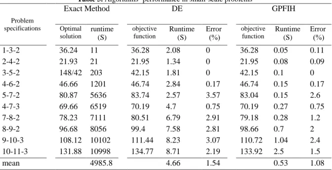
Table 3. A

Exact Method

Problem

specifications runtime (S) Optimal solution 11 36.24 1-3-2 21 21.93 2-4-2 203 148/42 3-5-2 1201 46.66 4-6-2 5636 80.87 5-7-2 6519 69.66 4-7-3 7111 78.23 7-8-2 8056 96.68 8-9-2 10102 108.12 9-10-3 10998 131.88 10-11-3 4985.8 mean

As can be seen in table 3, green PFIH heuristic algorithm and have a mean error of 1.08% and 1.54% and a

mean runtime of exact method is about 500 seconds. Figure 1 shows the performance of these algorithms in terms of runtime.

Figure 1. The performance of algorithms in terms of theirruntime for small

In figure 1, the right axis represents the runtime of the exact method. As it is clear, while problem size increases, the runtime of the exact method increases dramatically. It can also be seen that runtime of differential evaluation algorithm is more sensitive to the problem size than that of heuristic algorithm. 0 2 4 6 8 10 12

1 2 3

83

number of available vehicles. For example, 1-3-2 means: problem 1 where there are 3 customers

Algorithms’ performance in small-scale problems

DE Exact Method objective function Error (%) Runtime (S) objective function runtime 36.28 0 2.08 36.28 21.95 0 1.34 21.95 42.15 0 1.81 42.15 46.74 0.17 2.84 46.74 83.04 3.57 2.57 83.74 70.19 0.75 4.7 70.19 79.18 2.91 6.79 80.51 98.66 2.81 7.58 99.4 110.72 3.07 8.23 111.44 10102 133.92 2.19 8.71 134.77 10998 1.54 4.66 4985.8

le 3, green PFIH heuristic algorithm and differential evaluation algorithm have a mean error of 1.08% and 1.54% and a mean runtime of 0.53 and 4.66 seconds, while the mean runtime of exact method is about 500 seconds. Figure 1 shows the performance of these

The performance of algorithms in terms of theirruntime for small-scale problems

In figure 1, the right axis represents the runtime of the exact method. As it is clear, while e runtime of the exact method increases dramatically. It can also be seen that runtime of differential evaluation algorithm is more sensitive to the problem size than that of

4 5 6 7 8 9 10

EM DE GPFIH

2 means: problem 1 where there are 3 customers

GPFIH Error (%) Runtime (S) 0.11 0.05 0.09 0.08 0 0.1 0.17 0.15 2.6 0.15 0.75 0.27 1.2 0.28 2 0.7 2.4 1.04 1.5 2.5 1.08 0.53

differential evaluation algorithm mean runtime of 0.53 and 4.66 seconds, while the mean runtime of exact method is about 500 seconds. Figure 1 shows the performance of these

scale problems

In figure 1, the right axis represents the runtime of the exact method. As it is clear, while the e runtime of the exact method increases dramatically. It can also be seen that runtime of differential evaluation algorithm is more sensitive to the problem size than that of

0 2000 4000 6000 8000 10000 12000

(10)

84

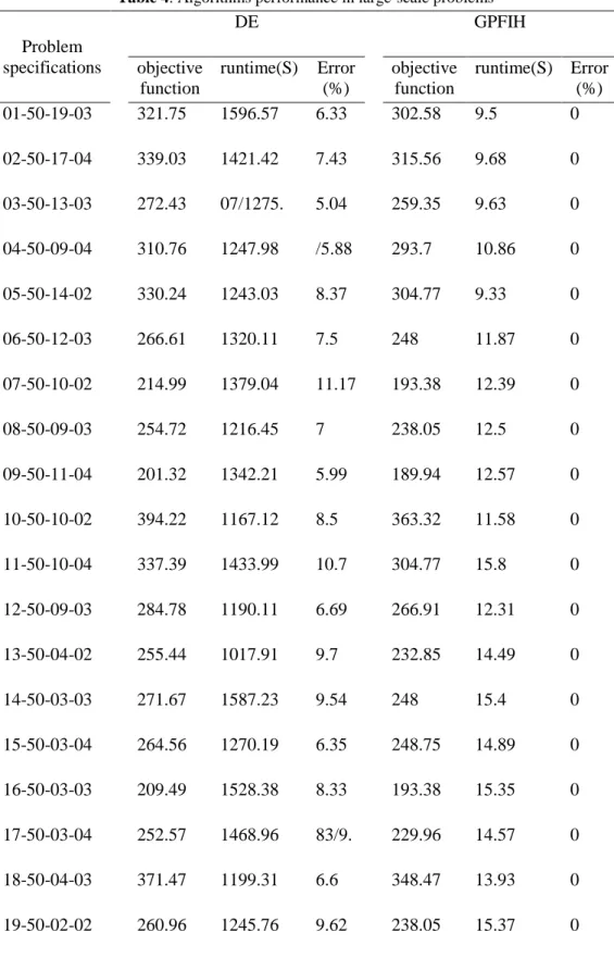
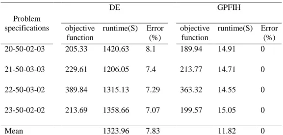
4-3- Evaluation of large-scale problems

In this section, 23 large-scale problems are solved five times by each algorithm. The average time and mean value of objective functions are presented in table 4.

Table 4. Algorithms performance in large-scale problems

GPFIH DE Problem

specifications Error

(%) runtime(S) objective function Error (%) runtime(S) objective function 0 9.5 302.58 6.33 1596.57 321.75 01-50-19-03 0 9.68 315.56 7.43 1421.42 339.03 02-50-17-04 0 9.63 259.35 5.04 07/1275. 272.43 03-50-13-03 0 10.86 293.7 /5.88 1247.98 310.76 04-50-09-04 0 9.33 304.77 8.37 1243.03 330.24 05-50-14-02 0 11.87 248 7.5 1320.11 266.61 06-50-12-03 0 12.39 193.38 11.17 1379.04 214.99 07-50-10-02 0 12.5 238.05 7 1216.45 254.72 08-50-09-03 0 12.57 189.94 5.99 1342.21 201.32 09-50-11-04 0 11.58 363.32 8.5 1167.12 394.22 10-50-10-02 0 15.8 304.77 10.7 1433.99 337.39 11-50-10-04 0 12.31 266.91 6.69 1190.11 284.78 12-50-09-03 0 14.49 232.85 9.7 1017.91 255.44 13-50-04-02 0 15.4 248 9.54 1587.23 271.67 14-50-03-03 0 14.89 248.75 6.35 1270.19 264.56 15-50-03-04 0 15.35 193.38 8.33 1528.38 209.49 16-50-03-03 0 14.57 229.96 83/9. 1468.96 252.57 17-50-03-04 0 13.93 348.47 6.6 1199.31 371.47 18-50-04-03 0 15.37 238.05 9.62 1245.76 260.96 19-50-02-02

(11)

85

GPFIH DE

Problem

specifications Error

(%) runtime(S) objective

function

Error (%) runtime(S) objective

function

0 14.91

189.94 8.1

1420.63 205.33

20-50-02-03

0 14.71

213.77 7.4

1206.05 229.61

21-50-03-03

0 14.55

363.32 7.29

1315.13 389.84

22-50-03-02

0 15.05

199.57 7.07

1358.66 213.69

23-50-02-02

0 11.82

7.83 1323.96

Mean

According to table 4, in this type of problems, modified PFIH algorithm performs better than differential evaluation algorithm. Modified PFIH algorithm have found better answers for all problems while differential evaluation algorithm has had an average of 7.83% error, a longer runtime and a slower convergence.

5- Conclusion

This paper proposed a PFIH-based heuristic algorithm called GPFIH which solves the vehicle routing problem with hard time windows while minimizing fuel consumption. The proposed heuristic used a novel speed optimization algorithm. Performance of the proposed algorithm was analyzed by comparing its results with the results of the exact method for small-scale problems and results of differential meta-heuristic for large-scale problems. In small-scale problems, green PFIH heuristic algorithm and differential evaluation algorithm had a mean error of 1.08% and 1.54% and a mean runtime of 0.53 and 4.66 seconds, respectively, while the mean runtime of the exact method was about 500 seconds. Solving 23 large-scale problems from those provided by Solomon showed that the mean error of the differential evaluation algorithm is 7.87% higher than that of green PFIH algorithm. Overall, the results indicated the good performance of the proposed algorithm.

References

Bektaş, T., & Laporte, G. (2011). The pollution-routing problem. Transportation Research Part B:

Methodological, 45(8), 1232-1250.

Berger, J., Barkaoui, M. and Bräysy, O.(2003). A Route-directed Hybrid Genetic Approach for the Vehicle Routing Problem with Time Windows. Information Systems and Operational Research, vol.41, 179-194.

Demir, E., Bektaş, T., & Laporte, G. (2014). The bi-objective pollution-routing problem. European

Journal of Operational Research, 232(3), 464-478.

Demir, E., Bektaş, T., & Laporte, G. (2012). An adaptive large neighborhood search heuristic for the pollution-routing problem. European Journal of Operational Research, 223(2), 346-359.

Erbao, C., & Mingyong, L. (2009). A hybrid differential evolution algorithm to vehicle routing problem with fuzzy demands. Journal of computational and applied mathematics, 231(1), 302-310.

(12)

86

Franceschetti, A., Honhon, D., Van Woensel, T., Bektaş, T., & Laporte, G. (2013). The time-dependent pollution-routing problem. Transportation Research Part B: Methodological, 56, 265-293.

Jeon, G., Leep, H. R., & Shim, J. Y. (2007). A vehicle routing problem solved by using a hybrid genetic algorithm. Computers & Industrial Engineering, 53(4), 680-692.

Kirby, H. R., Hutton, B., McQuaid, R. W., Raeside, R., & Zhang, X. (2000). Modelling the effects of transport policy levers on fuel efficiency and national fuel consumption. Transportation

Research Part D: Transport and Environment, 5(4), 265-282.

Koç, Ç., Bektaş, T., Jabali, O., & Laporte, G. (2014). The fleet size and mix pollution-routing problem. Transportation Research Part B: Methodological, 70, 239-254.

Lin, C., Choy, K. L., Ho, G. T., Chung, S. H., & Lam, H. Y. (2014). Survey of green vehicle routing problem: past and future trends. Expert Systems with Applications, 41(4), 1118-1138.

Lou, Y., Li, J., & Wang, Y. (2010, August). A Binary-Differential Evolution algorithm based on Ordering of individuals. In Natural Computation (ICNC), 2010 Sixth International Conference

on (Vol. 5, pp. 2207-2211). IEEE.

Marinakis, Y., Marinaki, M., & Spanou, P. (2015). A memetic differential evolution algorithm for the vehicle routing problem with stochastic demands. In Adaptation and hybridization in computational intelligence (pp. 185-204). Springer International Publishing.

Mingyong, L., &Erbao, C. (2010). An improved differential evolution algorithm for vehicle routing problem with simultaneous pickups and deliveries and time windows. Engineering Applications of Artificial Intelligence, 23(2), 188-195.

Prins, C. (2004). A simple and effective evolutionary algorithm for the vehicle routing problem. Computers & Operations Research, 31(12), 1985-2002.

Reimann, M., Doerner, K., & Hartl, R. F. (2004). D-ants: Savings based ants divide and conquer the vehicle routing problem. Computers & Operations Research, 31(4), 563-591.

Solomon, M.(1987). Algorithms for the vehicle routing and scheduling problems with time window constraints, Operations research, vol 35, 254-265

Storn, R., & Price, K. (1997). Differential evolution–a simple and efficient heuristic for global optimization over continuous spaces. Journal of global optimization, 11(4), 341-359.

Thangiah, S. R., Osman, I. H., & Sun, T. (1994). Hybrid genetic algorithm, simulated annealing and tabu search methods for vehicle routing problems with time windows. Computer Science

Department, Slippery Rock University, Technical Report SRU CpSc-TR-94-27, 69.

Toro, E., Franco, J., Echeverri, M., Guimarães, F., & Rendón, R. (2017). Green open location-routing problem considering economic and environmental costs. International Journal of Industrial Engineering Computations, 8(2), 203-216.