Modeling the effect of cost factors on productivity growth using data envelopment analysis

(1)

198

Modeling the effect of cost factors on productivity growth using

Data Envelopment Analysis

Mostafa Tavallaaee

1

, Fatemeh Rakhshan

2*

, Mohammad Reza Alirezaee

1,2 1_{Behin Kara Pajouh Institute of Operations Research, Tehran, Iran}

2_{School of Mathematics, Iran University of Science and Technology, Tehran, Iran}

[email protected], [email protected], [email protected]

Abstract

The role of some factors such as efficiency, rule and regulations, and balance have been already investigated in the context of productivity analysis based on data envelopment analysis models. Along with the studies that take the role of cost factors into account, this paper presents a novel four-component decomposition of Malmquist productivity growth index from a financial point of view. The cost efficiency model applied here uses assurance region weight restrictions to increase discrimination power of basic data envelopment analysis models. In the proposed decomposition, the proportion of cost efficiency changes during two time periods is determined as a quantity measure between zero and one. A real case study from banking industry including 66 branches located in east Tehran is employed to show the applicability of the proposed methods and the results were been analyzed.

Keywords: Data Envelopment Analysis, Malmquist index, cost efficiency, weight restrictions.

1-Introduction

Data envelopment analysis (DEA) is a mathematical programming technique for measuring and comparing the relative efficiency of decision-making units with multiple inputs and outputs which was put forward in the form of a linear programming model in 1978 (Charnes et al., 1978). This model is based on the constant return to scale (CRS) and is known as CCR. In 1984, Banker et al. (1984) extended the model to variable return to scale (VRS). Their model was named BCC. DEA is a field of operations research with many tools to estimate the efficiency of Decision Making Units (DMUs).

The Malmquist index is a concept which was first introduced by Malmquist in 1953 for input consumption analysis. In 1982, Caves et al. (1982) used the index for calculating productivity changes in two time periods, known as CCD formula. Then in 1992, Fare et al. (1992) combined the idea of calculating Farrell's efficiency and CCD formula for productivity to estimate the distance functions using DEA. They provided the first decomposition of the index known as FGLR: efficiency change (EC) and technology change (TC). Applying VRS technology in addition to CRS, Fare et al. (1994) presented a three-component decomposition referred to FGNZ: pure efficiency change (PEC), scale efficiency change (SEC), and technology change (TC). In 2010, the four-parted decomposition of extended Malmquist index was obtained by Alirezaaee and Afsharian (2010) using VRS and CRS technologies and input/output trade-offs: PEC, SEC, regulation efficiency change (REC) and extended technology change (ETC).

*Corresponding author

Journal of Industrial and Systems Engineering

Vol. 12, No. 4, pp. 198 - 207 Autumn (November) 2019

(2)

199

Afterwards Alirezaaee and Rajabi Tanha (2015) explored the balance concept for measuring to what extent units are aligned with the predefined strategies. Another four-parted decomposition of the extended Malmquist index (EMI) was obtained using VRS and CRS and balance model technologies: PEC, SEC, balance factor change (BFC) and ETC.

When we have input prices (or output prices for that matter) we can assess not only technical but also ‘cost efficiency’. In such a case we would measure the distance of each unit from a minimum cost frontier (Thanassoulis and Silva, 2018). Cost efficiency (CE) evaluates the ability to produce specific outputs with minimal cost. The concept of cost efficiency can be traced back to Farrell in 1957 who originated many of the ideas underlying DEA. Where producers are cost minimizers and input prices are known, a cost Malmquist productivity index were developed that decomposed into cost technical and allocative efficiency change and cost technical change (Maniadakis and Thanassoulis, 2004). But, it is defined in terms of cost rather than input distance functions. A cost Malmquist index also is proposed by Hosseinzadeh Lotfi et al. (2007) based on interval data and prices. The main contribution of the work of Camanho and Dyson (2005) consists of the development of a method for the estimation of upper and lower bounds for the CE measure in situations of price uncertainty, where only the maximal and minimal bounds of input prices can be estimated for each DMU. They also, proposed an equivalent CE model to Farrell's CE approach using Assurance Region type I (AR-I) weight restrictions in the presence of different scenarios consist of situations where input prices are known exactly at each DMU and situations with incomplete price information. Results of the review paper of Mardani (2017) indicate that DEA showed great promise to be a good evaluative tool for future analysis on energy efficiency issues, where the production function between the inputs and outputs was virtually absent or extremely difficult to acquire. To impose the law of one price (LoOP) restrictions, which state that all firms face the same input prices, Kuosmanen et al. (2006) developed the top-down and bottom-up approaches to maximizing the industry-level cost efficiency. However, the optimal input shadow prices generated by the above approaches need not be unique, which influences the distribution of the efficiency indices at the individual firm level. To solve this problem, in this paper, we developed a pair of two-level mathematical programming models to calculate the upper and lower bounds of cost efficiency for each firm in the case of non-unique LoOP prices while keeping the industry cost efficiency optimal (Fang & Li, 2015).

Venkatesh and Kushwaha (2016) considered short and long-run cost minimizing behavior of Indian public bus companies using CE model of DEA. Tohidi et al. (2017) proposed a global cost Malmquist productivity index, new cost Malmquist productivity index, that is circular and that gives a single measure of productivity change. A new cost Malmquist productivity index (CMPI) in multi-output settings with joint and output-specific inputs is presented by Walheer (2018). The cost Malmquist productivity index (CMPI) has been proposed to capture the performance change of cost minimizing Decision Making Units (DMUs). Recently, two alternative uses of the CMPI have been suggested: (1) using the CMPI to compare groups of DMUs, and (2) using the CMPI to compare DMUs for each output separately (Walheer, 2018). The paper supposes that the data and the costs are fixed and known and uses the model developed by Camanho and Dyson (2005). In fact, when the effect of cost efficiency topics is significant for different organizations such as banks, hospitals, educational systems, production firms, etc., using EMI finds necessity.

The remaining parts of the paper are organized as follows: section 2 presents a brief summary of DEA CE model. Section 3 introduces the extended MI (EMI). Section 4 illustrates the application of the model developed within the context of the case study of the 66 branches of bank Maskan located in east Tehran. Section 5 summaries and concludes.

2-Cost Efficiency in Data Envelopment Analysis

Based on Rakhshan et. al (2016), cost efficiency is one of the main approaches conducted by many DEA studies from 1957 until now. Cost efficiency reflects the ability of each DMU in production of the current outputs under minimal costs for the given price levels (Camanho and Dyson, 2008). In order to obtain a measure of cost efficiency, the minimum cost for the production the current level of outputs with

(3)

200

known input prices is obtained by solving the following linear problem, as first formulated by Fare et al. (1985):

min ∑ 𝑝𝑖0𝑥𝑖0 𝑚

𝑖=1

𝑠. 𝑡. ∑ 𝑥𝑖𝑗𝜆𝑗= 𝑥𝑖0, 𝑖 = 1, … , 𝑚, 𝑛

𝑗=1

(1)

∑ 𝑦𝑟𝑗𝜆𝑗≥ 𝑦𝑟0, 𝑟 = 1, … , 𝑠, 𝑛

𝑗=1

𝜆𝑗≥ 0, 𝑗 = 1, … , 𝑛

𝑥𝑖0≥ 0, 𝑖 = 1, … , 𝑚.

Assuming that 𝑝𝑖0 is the ith input price for DMU0 under evaluation, 𝑥_𝑖0∗ is the optimal input for DMU0 for producing the current amount of outputs at minimal costs. Then, the CE is obtained as the ratio of the minimal cost to the current cost as follows:

𝐶𝐸 =∑ 𝑝𝑖0𝑥𝑖0

∗ 𝑚 𝑖=1

∑𝑚𝑖=1𝑝𝑖0𝑥𝑖0

. (2)

Alternatively, the CE of DMU0 can be obtained by solving the following linear programming names CE model (CEM) which uses the AR-I weight restrictions attached to CCR model:

𝐶𝐸𝑀: max ∑ 𝑢𝑟𝑦𝑟0 𝑠

𝑟=1

𝑠. 𝑡. ∑ 𝑣𝑖𝑥𝑖0= 1, 𝑚

𝑖=1

∑ 𝑢𝑟𝑦𝑟𝑗− ∑ 𝑣𝑖𝑥𝑖𝑗 ≤ 0 𝑚

𝑖=1

, 𝑗 = 1, … , 𝑛,

𝑠

𝑟=1

(3)

𝑣𝑖𝑎 𝑣_𝑖𝑏 =

𝑝𝑖𝑎₀ 𝑝_𝑖𝑏₀, 𝑖

𝑎 _{< 𝑖}𝑏_{, 𝑖}𝑎_{, 𝑖}𝑏_{= 1, … , 𝑚,}

𝑢𝑟 ≥ 𝜀, 𝑟 = 1, … , 𝑠

Where 𝑣_𝑖𝑎 and 𝑣_𝑖𝑏 are the input weights corresponding to inputs 𝑖𝑎 and 𝑖𝑏. Also, 𝜀 is a non-Archimedian infinitesimal used to ensure that all inputs and outputs are taken into account for the efficiency assessment.

It can easily be shown that the above two models are equivalent. In the next section, we use this form of CE as the base technology in computing EMI. This model sets the relative values of the input weights as the relative values of the input prices observed in each DMU0.

3-Extended Malmquist Index

Here we intend to relate MI to the financial factors such as costs and calculate the effect of cost factor on the productivity growth. We have considered the cost as the baseline technology, which creates a

(4)

201

boundary that is placed out of CRS boundary. In the new extended index, not only the baseline of productivity growth is not functional and is based on the financial index of cost type, but rather obtains it from CE boundary instead of estimating the technology from the CRS boundary. The EMI differs from MI but, this difference is not such a way that brings into question the previous results, rather it somehow supplementary.

Using the CEM of (3) instead of CRS technology in CCD formula, we have the following definition of EMI:

𝐸𝑀𝐼𝐶𝐸𝑀 = [𝐷𝐶𝐸𝑀𝑡 (𝑥0𝑡+1,𝑦0𝑡+1)

𝐷_𝐶𝐸𝑀𝑡+1(𝑥₀𝑡_,𝑦 0𝑡) ×

𝐷_𝐶𝐸𝑀𝑡+1(𝑥₀𝑡+1_,𝑦 0𝑡+1)

𝐷_𝐶𝐸𝑀𝑡 (𝑥₀𝑡_,𝑦 0𝑡) ]

1 2 ⁄

₍₄₎

Where (𝑥₀𝑡, 𝑦0𝑡) and (𝑥0𝑡+1, 𝑦0𝑡+1) are the observed inputs and outputs of DMU0 in time periods 𝑡 and

𝑡 + 1 respectively. 𝐷𝐶𝐸𝑀𝑡 (𝑥0𝑡+1, 𝑦0𝑡+1) is calculated by solving model (3). Other measures in (4) are calculated in a similar manner.

[𝐷_𝐶𝐸𝑀𝑡 _(𝑥

0𝑡+1, 𝑦0𝑡+1)] = Max ∑ 𝑢𝑟𝑡𝑦𝑟0𝑡+1 𝑠

𝑟=1

𝑠. 𝑡. ∑ 𝑣𝑖𝑡𝑥𝑖0𝑡+1= 1 𝑚

𝑖=1

∑ 𝑢𝑟𝑡𝑦𝑟𝑗𝑡 𝑠

𝑟=1

− ∑ 𝑣_𝑖𝑡𝑥_𝑖𝑗𝑡 ≤ 0

𝑚

𝑖=1

, 𝑗 = 1, … , 𝑛

(5)

𝑣_𝑖𝑡𝑎 𝑣_𝑖𝑡𝑏

=𝑝𝑖𝑎0 𝑝_𝑖𝑏₀

, 𝑖𝑎 _{< 𝑖}𝑏_{, 𝑖}𝑎_{, 𝑖}𝑏 _{= 1, … , 𝑚,}

𝑢𝑟𝑡 ≥ 𝜀, 𝑟 = 1, … , 𝑠

Now we can develop other versions of EMI decompositions regarding CRS and CEM technologies. Two-component EMI can be written as

𝐸𝑀𝐼𝐶𝐸𝑀 _{= 𝐸𝐸𝐶}𝐶𝐸𝑀_{× 𝐸𝑇𝐶}𝐶𝐸𝑀₍₆₎ Where

𝐸𝐸𝐶𝐶𝐸𝑀 ₌𝐷𝐶𝐸𝑀 𝑡+1_(𝑥

𝑘𝑡+1, 𝑦𝑘𝑡+1)

𝐷_𝐶𝐸𝑀𝑡 _(𝑥 𝑘 𝑡_{, 𝑦}

𝑘𝑡)

, 𝐸𝑇𝐶𝐶𝐸𝑀 _{= [}𝐷𝐶𝐸𝑀

𝑡 _(𝑥

𝑘 𝑡+1_{, 𝑦}

𝑘𝑡+1)

𝐷_𝐶𝐸𝑀𝑡+1_(𝑥

×𝐷𝐶𝐸𝑀

𝑡 _(𝑥

𝑘 𝑡_{, 𝑦}

𝑘𝑡)

𝐷_𝐶𝐸𝑀𝑡+1_(𝑥 𝑘 𝑡_{, 𝑦}

𝑘𝑡)

]

1 2 ⁄

(7)

The novel three-component decomposition that specifies CEC portion in productivity index is developed regarding CRS technology and CEM as follows:

𝐸𝑀𝐼𝐶𝐸𝑀 = 𝐸𝐶 × 𝐶𝐸𝐶 × 𝐸𝑇𝐶𝐶𝐸𝑀 (8) Where

𝐸𝐶 =𝐷𝐶𝑅𝑆

𝑡+1_(𝑥

𝐷_𝐶𝑅𝑆𝑡 _(𝑥 𝑘 𝑡_{, 𝑦}

𝑘𝑡)

, 𝐶𝐸𝐶 =𝐶𝐸

𝑡+1_(𝑥

𝐶𝐸𝑡_(𝑥 𝑘 𝑡_{, 𝑦}

𝑘𝑡)

(9)

(5)

202 𝐷_𝐶𝑅𝑆𝑡 (𝑥_𝑘𝑡_{, 𝑦}

𝑘𝑡) = 𝑚𝑎𝑥 ∑ 𝑢𝑟𝑡𝑦𝑟𝑘𝑡 𝑠

𝑟=1

𝑠. 𝑡. ∑ 𝑣𝑖𝑡𝑥𝑖𝑘𝑡 𝑚

𝑖=1 = 1

𝑟=1 − ∑ 𝑣𝑖

𝑡_𝑥 𝑖𝑗𝑡 𝑚

𝑖=1 ≤ 0, 𝑗 = 1, … , 𝑛

(10)

𝑢𝑟𝑡 ≥ 𝜀, 𝑟 = 1, … , 𝑠

𝑣_𝑖𝑡 ≥ 𝜀, 𝑖 = 1, … , 𝑚

In addition, if we consider VRS technology in addition to CRS and CEM, other novel four-component decomposition of EMI will be obtained as follows:

𝐸𝑀𝐼𝐶𝐸𝑀 = 𝑃𝐸𝐶 × 𝑆𝐸𝐶 × 𝐶𝐸𝐶 × 𝐸𝑇𝐶𝐶𝐸𝑀, (11) Where PEC is obtained by solving BCC model as follows:

𝐷𝑉𝑅𝑆𝑡 (𝑥𝑘𝑡, 𝑦𝑘𝑡) = 𝑚𝑎𝑥 ∑ 𝑢𝑟𝑡𝑦𝑟𝑘𝑡 − 𝑢0 𝑠

𝑟=1

𝑠. 𝑡. ∑ 𝑣𝑖𝑡𝑥𝑖𝑘𝑡 = 1 𝑚

𝑖=1

𝑟=1

− ∑ 𝑣_𝑖𝑡𝑥_𝑖𝑗𝑡 − 𝑢0𝑡 ≤ 0 𝑚

𝑖=1

, 𝑗 = 1, … , 𝑛

(12)

𝑢𝑟𝑡 ≥ 𝜀, 𝑟 = 1, … , 𝑠, 𝑢0𝑡 free

𝑣𝑖𝑡 ≥ 𝜀, 𝑖 = 1, … , 𝑚 Also, we have

𝑆𝐸 =𝐷𝐶𝑅𝑆 𝐷𝑉𝑅𝑆

, 𝑆𝐸𝐶 =𝑆𝐸

𝑡+1_(𝑥 𝑘 𝑡+1_{, 𝑦}

𝑘𝑡+1)

𝑆𝐸𝑡_(𝑥 𝑘𝑡, 𝑦𝑘𝑡)

(13) We describe the above decompositions with an example:

Consider the data of 8 DMUs taken from Alirezaaee and Afsharian (2010) with one input and two outputs in two time periods, as in table 1.

Table 1. The data of 8 DMUs in two time periods Second period First period Units Output 2 Output 1 input Output 2 Output 1 input 700 600 400 1000 1000 2400 2100 2700 1100 1300 1500 1600 2800 900 4200 900 100 100 100 200 200 300 300 300 1000 600 100 800 600 2850 1200 2100 200 1200 1600 1000 2600 300 3600 2100 100 100 100 200 200 300 300 300 DMU 1 DMU 2 DMU 3 DMU 4 DMU 5 DMU 6 DMU 7 DMU 8

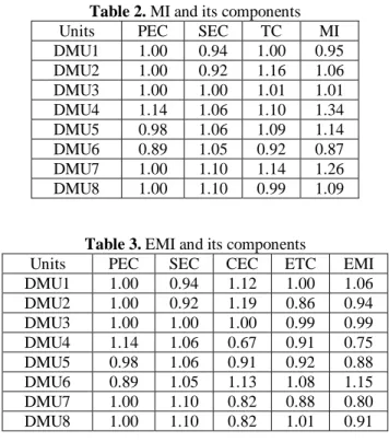
The results of MI and EMI with their decompositions using GAMS programming is shown in tables 2 and 3.

(6)

203

Table 2. MI and its components

Units PEC SEC TC MI

DMU1 1.00 0.94 1.00 0.95

DMU2 1.00 0.92 1.16 1.06

DMU3 1.00 1.00 1.01 1.01

DMU4 1.14 1.06 1.10 1.34

DMU5 0.98 1.06 1.09 1.14

DMU6 0.89 1.05 0.92 0.87

DMU7 1.00 1.10 1.14 1.26

DMU8 1.00 1.10 0.99 1.09

Table 3. EMI and its components

Units PEC SEC CEC ETC EMI

DMU1 1.00 0.94 1.12 1.00 1.06

DMU2 1.00 0.92 1.19 0.86 0.94

DMU3 1.00 1.00 1.00 0.99 0.99

DMU4 1.14 1.06 0.67 0.91 0.75

DMU5 0.98 1.06 0.91 0.92 0.88

DMU6 0.89 1.05 1.13 1.08 1.15

DMU7 1.00 1.10 0.82 0.88 0.80

DMU8 1.00 1.10 0.82 1.01 0.91

Comparing the three-parted and four-parted decompositions, PEC and SEC are clearly common in both of them and remain unchanged. Therefore, we need to focus on technological changes as well as on CEC effect as a new component.

In the three-parted decomposition, the effect of technology on PEC and SEC is considered, while in the four-parted decomposition, a new factor titled the cost efficiency along with the technological changes, increase the accuracy of results and help the managers in providing an effective developmental solution for their units. As shown in tables 2 and 3, in DMUs 1 and 6, comparing MI and EMI and considering the CEC factor, their status has been changed from unproductive to productive ones. On the other hand, the DMUs 4 and 7 are unproductive units, as the rate of cost efficiency growth is negative for them; in other words, by applying MI, the negative growth in technology change might lead to negative growth of productivity, while by using the four-parted decomposition it precisely estimates that whether the negative growth results from negative growth of CEC or is due to technology change.

4-Case study

In this section, we calculate and analyze the proposed EMI novel decompositions for 66 branches of an expertise bank in Iran located in east region of Tehran for two time periods 2017-2018 as a real-world case study. It is noted that the chosen bank is the largest Iranian governmental bank operating in the housing sector. This bank has more than 1300 branches in 38 regions in Iran.

4-1-Data

Considering the production approach of bank branches (Paradi and Zhu, 2013), two inputs and three outputs are considered as follows: Human resources and location index are inputs and deposits, loans and services are outputs in this case study.

The input of human resources has to include all the quantities and qualities entities related to the staff of a branch. The input of location has to include all the quantities and qualities entities related to the physical location of a branch. The planning and programming department of bank has done a project for this index and they considered all the related factors in the developed location index and we used the data of the location index in our evaluation.

(7)

204

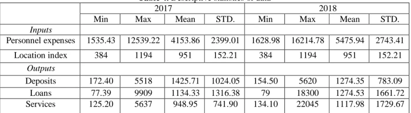
The output of deposit has to include all kinds of methods of gathering money by a branch. The planning and programming department of bank has done a project for this index and they considered a weighted sum of all kinds of accounts considering their values and number of transactions for calculation of the deposit index and we used the data of the deposit index in our evaluation. The output of loans includes all the money gave as all kinds of loans and mortgages by a branch and similar to deposit index some calculations have been done. Finally the output of services is an index which includes all kinds of services presented by a branch to its customers. Descriptive statistics of inputs and outputs for two time periods are given in Table 4. Measurement unit of personnel expenses is 1000000 Rials. Other indices have no units because they are normalized indices. All the values and results are rounded in two digits.

Table 4. Descriptive statistics of data

2017 2018

Min Max Mean STD. Min Max Mean STD.

Inputs

Personnel expenses 1535.43 12539.22 4153.86 2399.01 1628.98 16214.78 5475.94 2743.41

Location index 384 1194 951 152.21 384 1194 951 152.21

Outputs

Deposits 172.40 5518 1425.71 1024.05 154.50 5620 1274.35 783.09

Loans 77.39 9909 1134.33 1316.38 79 18300 1274.53 1661.72

Services 125.20 5637 948.95 741.90 134.10 22045 1117.98 1729.67

Also, descriptive statistics of input costs are given in table 5. P1 is the cost of human resources that is replaced by personnel expenses which contain all expenses related to staff of branch such as pay, pension and etc. P2 is the cost of the project for implementing and computing location index for each branch. Since the cost information is used in the form of proportion in the model, so their relative value is only important.

Table 5. Descriptive statistics of input costs

2017 2018

Min Max Mean STD. Min Max Mean STD.

P1 1.00 5.10 1.71 0.91 1.00 6.00 2.18 1.20

P2 2.00 5.00 3.84 0.68 2.00 5.00 3.84 0.68

4-1-Extended Malmquist index results

Both MI and EMI with their components were calculated for all branches. Since expressing the results for all 66 branches is not possible, we only provide descriptive statistics of the results for all branches and the results for selected branches. Descriptive results are listed in table 6.

Table 6. Descriptive statistics of MI and EMI decompositions

Min Max Mean STD.

PEC 0.57 1.36 1.03 0.16

SEC 0.51 1.63 0.98 0.15

TC 0.69 1.48 1.04 0.16

ETC 0.68 1.15 0.90 0.09

CEC 0.38 3.86 1.19 0.49

MI 0.69 1.77 1.02 0.17

(8)

205

Now, regarding increasing or decreasing EMI relative to MI in all 66 branches, we divide them into three groups: branches with EMI-MI>0, EMI-MI<0, and EMI-MI≈0. Then analyze the three groups performance separately.

 Branches with EMI-MI>0:

27 branches located in this group. Between them, the branches 2, 5, 16, 29, 34, 47, 49 have the largest value for EMI-MI that is listed in table 7. Considering the CEC, these branches show a higher productivity index than MI. For example, the dramatic growth of EMI of branch #2 relative to MI is due to CEC that is equal to 1.66. It means that CE of the branch has 66% growth in the two periods. Also, the same analysis is possible for other branches in table 7.

Table 7. The results for Branches with highest EMI-MI

DMUs PEC SEC TC MI EMI ETC CEC

DMU02 1.00 1.00 0.70 0.69 1.41 0.85 1.66 DMU05 1.00 1.00 0.72 0.72 1.41 0.90 1.58 DMU16 1.00 0.51 1.48 0.75 1.33 0.68 3.87 DMU29 0.94 1.00 0.85 0.79 1.24 0.72 1.84 DMU34 0.90 1.00 0.77 0.70 1.41 0.84 1.86 DMU47 0.98 0.99 0.77 0.74 1.31 0.89 1.50 DMU49 0.75 1.00 0.93 0.70 1.40 0.94 1.94

Note that the value of PEC and SEC are equal in both decompositions MI and EMI. The changes of EMI relative to MI are due to growth or decline of CEC or ETC relative to TC.

 Branches with EMI-MI<0:

Among 21 branches belong to this group, the branches 7,14,22,39,45,51,66 have the lowest value of EMI-MI that are listed in table 8.

Table 8. The results for Branches with lowest EMI-MI

DMU07 1.27 0.99 1.01 1.27 0.78 0.99 0.63 DMU14 1.03 1.02 1.06 1.11 0.69 0.81 0.82 DMU22 1.36 0.91 1.09 1.35 0.63 0.83 0.62 DMU39 1.15 0.91 1.15 1.21 0.82 0.86 0.91 DMU45 0.93 0.97 1.34 1.21 0.82 0.74 1.22 DMU51 1.05 1.01 1.17 1.24 0.80 0.85 0.89 DMU66 1.00 1.63 1.09 1.77 0.56 0.92 0.38

As can be seen from table 8, the reason of decreasing EMI relative to MI is due to negative rate of ETC or CEC. For example, the decline of EMI relative to MI of branch #7 is due to negative growth of CEC that is equal to 0.63.

 Branches with EMI-MI≈0:

Regardless of efficient or inefficient, 18 branches have no significant relative changes in EMI. Among them, for example, we consider branches number 8, 15, 26, 27, 33, and 61. The results for these branches are given in table 9 below. In these branches, the CEC and ETC have compensated each other. In other words, the negative growth of CEC is offset by the positive growth of ETC and vice versa. For example, branch #8 has 62% growth in CEC and in other hand 52% decrease in ETC relative to TC.

(9)

206

Table 9. The results for Branches with EMI-MI≈0

DMU08 1.00 0.79 1.30 1.01 0.99 0.78 1.62 DMU15 0.98 0.98 1.05 1.00 1.00 0.95 1.09 DMU26 1.13 0.94 0.97 1.03 0.97 1.03 0.89 DMU27 1.11 0.95 0.95 1.00 1.00 1.03 0.91 DMU33 0.96 1.00 1.05 1.02 0.98 0.96 1.06 DMU61 0.66 1.31 1.17 1.01 0.99 0.85 1.34

Since in both decompositions of MI and EMI, the components of SEC and PEC are the same, therefore it can be concluded that for these branches, the product of ETC with CEC is approximately equal to TC. The importance of CE analysis is more apparent in branches that have MI<0 but EMI>0, or MI>0 but EMI<0. This means that the CEC could make the branch's status be changed from non-productive to productive or vice versa.

5-Conclusion

The cost information of each decision making unit made us to develop a new extension of Malmquist productivity index that determine the role of cost efficiency changes in productivity growth or decline in two time periods. This paper applies the DEA cost efficiency model as the base technology and presents a four-component decomposition of Malmquist index. The cost efficiency model uses weight restrictions to increase discrimination power of basic DEA models. Finally, we approved the models presented in the paper with a real case study from banking industry with 66 branches. The results show that the extended decomposition provides more accurate analysis of contribution of each factor of technology change, efficiency change, and cost efficiency change in productivity growth index.

As a future work offer, one can consider the role of profit or revenue efficiency in productivity analysis. Also, VRS technology instead of CRS technology could be used.

References

Alirezaee, M. R., & Afsharian, M. (2010). Improving the discrimination of data envelopment analysis models in multi time periods. International Transactions in Operational Research, 17(5), 667-679. Alirezaee, M. R., & Tanha, M.R. (2015). Extending the Malmquist index to consider the balance factor of decision making units in a productivity analysis. IMA Journal of Management Mathematics, 27(3), 1-14. Banker, R. D., & Charnes, A., Cooper, W.W. (1984). Some models for estimating technical and scale inefficiency in data envelopment analysis. Management Science, 30(9), 1078-1092.

Camanho, A. S., & Dyson, R. G. (2005). Cost efficiency measurement with price uncertainty: a DEA application to bank branch assessment. European Journal of Operational Research, 161(2), 432-460. Camanho, A.S., & Dyson, R. G. (2008). A generalization of the Farrell cost efficiency measure applicable to non-fully competitive settings. Omega, 36(1),147-162.

Caves, D. C., Christensen, L. R., & Dievert, W. E. (1982). The economic theory of index number and the measurement of input, output, and productivity. Econometrica, 50(6), 1393-1414.

Charnes, A., Cooper, W. W., & Rhodes, E. (1978). Measuring the efficiency of the decision making units.

European Journal of Operational Research, 2(6), 429-444.

Fang, L., & Li, H., (2015). Cost efficiency in data envelopment analysis under the law of one price.

(10)

207

Fare, R., Grosskopf, S., Lindgren, B., & Roose, P. (1992). Productivity change in Swedish analysis pharmacies (1980-1989) a nonparametric Malmquist approach. Journal of Productivity, 3, 85-102.

Fare, R., Grosskopf, S., Norris, M., & Zhang, A. (1994). Productivity growth, technical progress, and efficiency changes in industrial country. AmericanEconomic Review, 84(1), 66-83.

Farrall, M. J. (1957). The measurement of productive efficiency. Journal of the Royal Statistical Society,

Series A 120, 253-81.

Kuosmanen T, L Cherchye and T Sipilainen (2006). The Law of One Price in Data Envelopment Analysis: Restricting Weight Flexibility across Firms. European Journal of Operational Research,

170(3), 735-757.

Maniadakis, N., & Thanassoulis, E. (2004). A cost Malmquist productivity index. European Journal of Operational Research, 154(2), 396-409.

Mardani, A., Zavadskas, E. K., Streimikiene, D., Jusoh, A., & Khoshnoudi, M., (2017). A comprehensive review of data envelopment analysis (DEA) approach in energy efficiency, Renewable and Sustainable Energy Reviews, 70(3), 1298-1322.

Rakhshan, F., Alirezaee, M., Modirii, M., & Iranmanesh, M. (2016). An Insight into the Model Structures Applied in DEA-Based Bank Branch Efficiency Measurements. Journal of Industrial and Systems Engineering, 9(2), 38-53.

Thanassoulis, E., & Silva, M. C. A., (2018). Measuring Efficiency Through Data Envelopment Analysis, Impact, 2018(1), 37-41.

Tohidi, G., Razavyan, S., & Tohidnia, S., (2012). A global cost Malmquist productivity index using data envelopment analysis, Journal of the Operational Research Society, 63(1), 72-78.

Venkatesh, A., & Kushwaha, S., (2018). Short and long-run cost efficiency in Indian public bus companies using Data Envelopment Analysis. Socio-Economic Planning Sciences, 61(3), 29-36.

Walheer, B., (2018). Disaggregation of the cost Malmquist productivity index with joint and output-specific inputs, Omega, 75(3), 1-12.

Walheer, B., (2018). Cost Malmquist productivity index: an output-specific approach for group comparison. Journal of productivity analysis, 49(1), 79-94.