arXiv:1704.01820v1 [cond-mat.soft] 6 Apr 2017
Anupam Pandey,1,∗ Stefan Karpitschka,1 Luuk A. Lubbers,2 Joost H. Weijs,3 Lorenzo Botto,4 Siddhartha Das,5 Bruno Andreotti,6 and Jacco H. Snoeijer1, 7
1
Physics of Fluids Group, Faculty of Science and Technology, University of Twente, P.O. Box 217, 7500AE Enschede, The Netherlands
2
Huygens-Kamerlingh Onnes Lab, Universiteit Leiden, P.O. Box 9504, 2300RA Leiden, The Netherlands
3
Universit´e Lyon, Ens de Lyon, Universit´e Claude Bernard, CNRS, Laboratoire de Physique, F-69342 Lyon, France
4
School of Engineering and Materials Science, Queen Mary University of London, London E1 4NS, UK
5
Department of Mechanical Engineering, University of Maryland, College Park, MD 20742, USA
6
Laboratoire de Physique et M´ecanique des Milieux Het´erog`enes, UMR 7636 ESPCI- CNRS, Universit´e Paris- Diderot, 10 rue Vauquelin, 75005 Paris, France
7
Department of Applied Physics, Eindhoven University of Technology, P.O. Box 513, 5600MB Eindhoven, The Netherlands
(Dated: April 7, 2017)
Recent experiments have shown that liquid drops on highly deformable substrates exhibit mutual interactions. This is similar to the Cheerios effect, the capillary interaction of solid particles at a liquid interface, but now the roles of solid and liquid are reversed. Here we present a dynamical theory for this inverted Cheerios effect, taking into account elasticity, capillarity and the viscoelastic rheology of the substrate. We compute the velocity at which droplets attract, or repel, as a function of their separation. The theory is compared to a simplified model in which the viscoelastic dissipation is treated as a localized force at the contact line. It is found that the two models differ only at small separation between the droplets, and both of them accurately describe experimental observations.
I. INTRODUCTION
The clustering of floating objects at the liquid inter-face is popularly known as the Cheerios effect [1]. In the simplest scenario, the weight of a floating particle deforms the liquid interface and the liquid-vapor surface tension prevents it from sinking [2]. A neighboring par-ticle can reduce its gravitational energy by sliding down the interface deformed by the first particle, leading to an attractive interaction. The surface properties of par-ticles can be tuned to change the nature of interaction, but two identical spherical particles always attract [3]. Anisotropy in shape of the particles or curvature of the liquid interface adds further richness to this everyday phenomenon [4–6]. Self-assembly of elongated mosquito eggs on the water surface provides an example of this capillary interaction in nature [7], while scientists have exploited the effect to control self-assembly and pattern-ing at the microscale [8–12].
The concept of deformation-mediated interactions can be extended from liquid interfaces to highly deformable solid surfaces. Similar to the Cheerios effect, the weight of solid particles on a soft gel create a depression of the substrate, leading to an attractive interaction [13–15]. Recently, it was shown that the roles of solid and liq-uid can even be completely reversed: liqliq-uid drops on soft gels were found to exhibit a long-ranged interaction, a phenomenon called theinverted Cheerios effect [16]. An example of such interacting drops is shown in fig. 1(a). In
this case, the droplets slide downwards along a thin, de-formable substrate (much thinner as compared to drop size) under the influence of gravity, but their trajecto-ries are clearly deflected due to a repulsive interaction between the drops. Here capillary traction of the liquid drops instead of their weight deforms the underlying sub-strate (cf fig. 1(b)). The scale of the deformation is given by the ratio of liquid surface tension to solid shear modu-lus (γ/G), usually called the elasto-capillary length. Sur-prisingly, drops on a thick polydimethylsiloxane (PDMS) substrate (much thicker than the drop sizes) were found to always attract and coalesce, whereas for a thin sub-strate (much thinner than the drop sizes) the drop-drop interaction was found to be repulsive [16]. This inter-action has been interpreted as resulting from the local slope of the deformation created at a distance by one drop, which can indeed be tuned upon varying the sub-strate thickness.
Here we wish to focus on the dynamical aspects of the substrate-mediated interaction. Both the Cheerios effect and the inverted Cheerios effect are commonly quantified by an effective potential, or equivalently by a relation between the interaction force and the particle separation distance [1, 16]. However, the most direct manifestation of the interaction is the motion of the particles, mov-ing towards or away from each other. In the example of fig. 1(a), the dark gray lines represent drop trajec-tories and the arrows represent their instantaneous ve-locities. When drops are far away, the motion is purely vertical due to gravity with a steady velocity ~vg. As
x
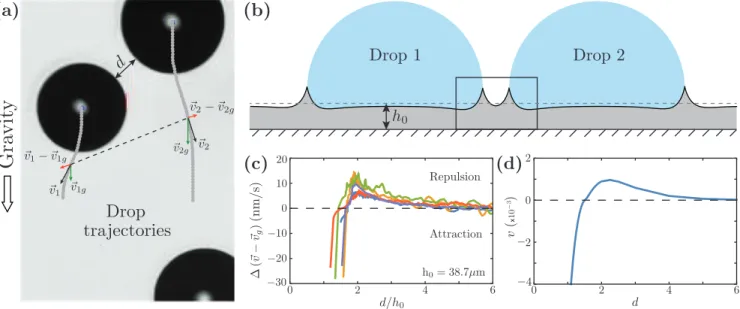
FIG. 1. Dynamics of the inverted cheerios effect. (a) Ethylene glycol drops of radiusR≃0.5−0.8 mm move down a vertically placed cross-linked PDMS substrate of thickness h0 ≃.04 mm and shear modulus G = 280 Pa under gravity. The arrows represent instantaneous drop velocity. Drop trajectories deviate from straight vertical lines due to a repulsive interaction between them. (b) A sketch of the cross-section of two drops on a thin, soft substrate. The region around two neighboring contact lines is magnified in fig. 2(a). (c) Relative interaction velocity as a function of the gapdbetween drops for five pairs of drops. We use the convention that a positive velocity signifies repulsion and negative velocity signifies attraction. (d) A theoretical velocity-distance plot for power-law rheology.
i = 1,2) that move the drops either away or towards each other. In fig. 1(c), we quantify the interaction by ∆(~v−~vg) = (~v1−~v1g)−(~v2−~v2g), representing the
relative interaction velocity as a function of inter drop distance (d) for several interaction events. Even though the dominant behavior is repulsive, we find an attractive regime at small distances. Similar to the drag force on a moving particle at a liquid interface [17], viscoelastic properties of the solid resist the motion of liquid drops on it [18]. Experiments performed in the over damped regime allow one to extract the interaction force from the trajectories, after proper calibration of the relation for the drag force as a function of velocity [16].
In this paper, we present a dynamical theory of elasto-capillary interaction of liquid drops on a soft substrate. For large drops, the problem is effectively two dimen-sional (cf. fig. 1(b)) and boils down to an interaction be-tween two adjacent contact lines. By solving the dynam-ical deformation of the substrate, we directly compute the velocity-distance curve based on substrate rheology, quantifying at the same time the interaction mechanism and the induced dynamics. In sec. II we set up the for-mulation of the problem and propose a framework to in-troduce the viscoelastic properties of the solid. In sec. III we present our main findings in the form of velocity-distance plots for the case of very large drops. These results are compared to the previous theory for force-distance curves, and we investigate the detailed structure of the dynamical three phase contact line. Subsequently, our results are generalised in sec. IV to the case of finite-sized droplets, and a quantitative comparison with
ex-periments is given.
II. DYNAMICAL ELASTOCAPILLARY INTERACTION
A. Qualitative description of the interaction mechanism
assumeγsv=γsℓ=γs.
To understand the interaction mechanism, we mag-nify the deformation around neighbouring contact lines in fig. 2(a). It shows a sketch of two repelling contact lines with velocity v. Our goal is to find the value of v for a given distanced. Deformation of the substrate at the three phase contact line is fully defined by the balance of three respective surface tensions, known as the Neumann condition [19–21]. The assumption of γsv = γsℓ = γs
leads to the symmetric wetting ridges of fig. 2(a). As demonstrated in the next section, in first approximation the solid profile is obtained by the superposition of the deformations due to the two moving contact lines shown in fig. 2b. However, motion on a viscoelastic medium causes a rotation of the wetting ridge by an angle φv
that depends on the velocity: the larger the velocity, the larger the rotation angle [22]. At the same time, super-position results in a rotation of a wetting ridge due to the local slope of the other deformation profile (H′
−v(d)) at
that location. Hence, the force balance with the capillary traction from an unrotated liquid interface can be main-tained when both rotations exactly cancel each other. Therefore, by equating H′
−v(d) toφv, we obtain a
rela-tion between velocity and distance.
B. Formulation
In this section, we calculate the dynamic deformation of a linear, viscoelastic substrate below a moving contact line. This step will enable us to quantify the interaction velocity, according to the procedure described above.
Due to the time-dependent relaxation behaviour of vis-coelastic materials, the response of the substrate requires a finite time to adapt to any change in the imposed trac-tion at the free surface. Under the assumptrac-tion of linear response, the stress-strain relation of a viscoelastic solid is given by [23]
σ(x, t) = ˆ t
−∞
dt′Ψ(t−t′) ˙ǫ(x, t′)−p(x, t)I. (1)
Here σ is the stress tensor, ǫ is the strain tensor, Ψ is the relaxation function, p is the isotropic part of the stress tensor, I is the identity tensor, and x = {x, y}. Throughout we will assume plain strain conditions, for which all strain components normal to the page vanish. We are interested in the surface profile of the deformed substrate, given by the vertical (y)-component of dis-placement vector u. For small deformations this imply
uy(x, h0, t) = h(x, t). The soft substrate is attached to a rigid support at its bottom surface and subjected to tractionT(x, t) on the top surface due to the pulling of the contact line. In addition, the surface tension of the solid γs provides a solid Laplace pressure that acts as
an additional traction on the substrate. For inertia-free dynamics, the Cauchy equation along with the boundary conditions for the plane strain problem are given by
FIG. 2. Illustration of the interaction mechanism. (a) Schematic representation of the deformed substrate due to a repulsive interaction between two contact lines. (b) Dy-namic deformation profiles associated to each of the contact line. Superposition of these two profiles give the resultant deformation.
∇.σ= 0, (2a)
σyy|y=h0 =T(x, t) +γs∂
2h
∂x2, (2b)
σyx|y=h0= 0, (2c)
u(x,0, t) = 0. (2d)
Following previous works [22, 24], we solve eqns. (1) and (2) using a Green’s function approach. Applying Fourier transforms in both space and time (x→qnoted by ‘˜’,t→ω noted by ‘ˆ’), the deformation can be writ-ten as,
b e
h(q, ω) =Tbe(q, ω)
"
γsq2+
µ(ω)
e K(q)
#−1
. (3)
Forward and backward Fourier transforms (with re-spect to space) of any function is defined as, fe(q) = ´∞
−∞f(x)e
−iqxdxandf(x) =´∞ −∞fe(q)e
iqxdq/2π.
Trans-formation rules are equivalent for t ↔ ω. Here µ(ω) is the complex shear modulus of the material and consists of the storage modulusG′(ω) =ℜ[µ(ω)], and loss modu-lusG′′(ω) =ℑ[µ(ω)]:
µ(ω) = iω
ˆ ∞
0
The spatial dependence is governed by the kernelKe(q), which for an incompressible, elastic layer of thicknessh0 reads
e K(q) =
sinh(2qh0)−2qh0 cosh(2qh0) + 2(qh0)2+ 1
1
2q. (5)
Two backward transforms of (3) give the surface defor-mationh(x, t).
In what follows, we perform the calculations assuming a power-law rheology of the soft substrate, characterised by a complex modulus,
µ(ω) =G[1 + (iωτ)n]. (6) This rheology provides an excellent description of the reticulated polymers like PDMS, as are used in exper-iments on soft wetting [22, 25–27]. In particular, the loss modulus has a simple power-law form, G′′ ∼ G(ωτ)n,
where Gis the static shear modulus and τ is the relax-ation timescale. The exponent n depends on the stoi-chiometry of the gel, and varies between 0 and 1 [28–30]. The experimental data presented in fig. 1 is for a PDMS gel with a measured exponent ofn= 0.61 and timescale
τ= 0.68s.
C. Two steadily moving contact lines
Now we turn to two moving contact lines, as depicted in fig. 2(a). Laplace pressure of the liquid drops scales withR−1, and vanish in this limit of large drops. Hence, the applied traction is described by two delta functions (notedδ), separated by a distanced(t):
T(x, t) =γδ
x+d(t) 2
+γδ
x−d(t)
2
. (7)
Owing to the linearity of the governing equations, the deformations form a simple superposition
h(x, t) =h1(x, t) +h2(x, t). (8)
Here h1(x, t) and h2(x, t) respectively are the solutions obtained for contact lines moving to the left and right.
Before considering the superposition, let us first discuss the deformation due to a contact line centered at the ori-gin and moving steadily with velocity−v. The traction and deformation are then of the form γδ(x+vt), and
H−v(x+vt). When computing the shape in a co-moving
frame, it can be evaluated explicitly from (3) as
e
H−v(q) =γ
"
γsq2+
µ(vq)
e K(q)
#−1
. (9)
The effect of velocity is encoded in the argument of the complex modulusµ, and hence couples to the dissipation
inside the viscoelastic solid. Settingv = 0, this expres-sion (9) gives a perfectly left-right symmetric deforma-tion of the contact line. As argued, forv6= 0, the motion breaks the left-right symmetry and induces a rotation of the wetting ridge.
Now, for two contact lines located at±d(t)/2 moving quasi-steadily with opposite velocitiesv =±12d˙, the de-formation in eq. (8) can be written as
h(x, t) =H−v
x+d 2
+Hv
x−d
2
. (10)
Under this assumption of quasi-steady motion, there is no explicit time-dependence; the shape is fully known once the velocityvand the distance dare specified. However, as discussed in sec. IIA, the total deformation of eq. (10) should be consistent with a liquid angle of π/2. This is satisfied when the ridge rotation due to motion, φv,
perfectly balances the slope induced by the second drop. Summarizing this condition as
H−′v(d) =φv, (11)
we can compute the velocityv for given separationdof the two contact lines. Explicit expressions can now be found from equation (9), as
H−′v(d) =
ˆ ∞
−∞
iqHe−v(q)eiqddq
2π, (12)
and (See ‘Methods’ section of [22] for details)
φv=−
1 2
H′
v 0+
+H′
v 0−
=−
ˆ ∞
−∞
ℜhiqHev(q)
idq
2π.
(13)
In what follows we numerically solve eq. (11), and obtain the interaction velocity as a function ofd.
D. Dimensionless form
The results below will be presented in dimensionless form. We use the substrate thicknessh0 as the charac-teristic lengthscale, relaxation timescale of the substrate
τ as the characteristic timescale, and introduce the fol-lowing dimensionless variables:
q=qh0, x= x
h0
, H= H
h0
, d¯= d
h0
, ¯v= vτ
h0
,
ω=ωτ, Ke= Ke
h0
, He = He
h2 0
, µ= µ
G.
(14)
reads
e
H−v(q) =α
"
αsq2+
µ(vq)
e K(q)
#−1
, (15)
This form suggests that the two main dimensionless pa-rameters of the problem are,
α= γ
Gh0
, αs=
γs
Gh0
, (16)
which can be seen as two independent elastocapillary numbers. αcompares the typical substrate deformation to its thickness, and as discussed in the next section αs
measures the decay of substrate deformation compared to
h0. The assumption of linear (visco)elasticity demands that the typical slope of the deformation is small, which requires α/αs =γ/γs ≪1. In the final section we will
also consider drops of finite sizeR. In that case, the ratio
R/h0appears as a third dimensionless parameter.
III. RESULTS
A. Relation between velocity and distance
Here we discuss our main result, namely the contact line velocityv of the inverted Cheerios effect, as a func-tion of distance d. Figure 1(d) represents a typical velocity-distance plot for αs = 1 and n = 0.7 obtained
by numerically solving eq. (11). The theory shows qual-itative agreement with the experiments: the interaction velocity is repulsive at large distance, but displays an at-traction at small distances. The change in the nature of interaction can be understood from the local slope of deformation. As can be seen from fig. 2(b), the slope
H′
−vis negative at small distances from the contact line.
This induces a negative velocity (attraction) to the con-tact line located at d/2. However, incompressibility of the material causes a dimple around the wetting ridge, and atd∼1 the slope changes its sign and so does the interaction velocity. A fully quantitative comparison be-tween theory and experiment, taking into account finite drop size effects, will be presented at the end of the paper in Sec. V.
We now study the velocity-distance relation in more detail. In fig. 3(a), we show the interaction velocity on a semi-logarithmic scale, for different values of the rheolog-ical parametern. In all cases the interaction is attractive at small distance, and repulsive at large distance. The point where the interaction changes sign is identical for all these cases. The straight line at larged reveals that the interaction speed decays exponentially, v ∼ e−λd.
The exponentλis not universal, but varies asλ∼1/n. Indeed by rescaling the velocity as |v|n, we observed a
collapse of the curves (cf. fig. 3(b)) in the ranges where the interaction velocities are small. The inset of fig. 3(b),
FIG. 3. (a) velocity-distance plots for increasing n values (n=0.5, 0.6, 0.7, 0.9), for the parameter αs = 1. The red
dashed line represent the far-filed asymtotic given in eq. (20) forn= 0.7. (b) Rescaling the velocity gives a perfect collapse for small velocity (large distance). Inset: rescaled velocity vs distance on a log-log plot. The prefactor A(n) is given by A(n) =n2n−1
/cos(nπ/2).
however, shows that the collapse does not hold at very small distances where the velocities are larger.
To understand these features, we extract the far-field asymptotics of the velocity-distance curve. As v de-creases for large d, we first expand eq. (12) for small
vto get
H−′ v≃α
ˆ ∞
−∞ iq
"
αsq2+ 1
e K(q)
#−1 eiqddq
2π +O(v). (17)
This effectively corresponds to the slope of a stationary contact line and the viscoelastic effects drop out. Hence, at large distances away from the contact line the de-formed shape is essentially static. The substrate elas-tocapillary number (αs) governs the deformed shape in
far field. In the Appendix we evaluate this static slope, which yields
H−′v ≃α C(αs) e−eλ(αs)d, (18)
indeed providing an exponential decay. This relation con-firms thatαsgoverns the decay of substrate deformation.
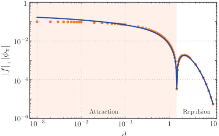
FIG. 4. Force vs distance plot forα= 1/5 andαs= 1. The
blue line represents the dissipative drag force forn= 0.7 given in eq. (13). The red points represent the localized force given by eq. (21). Beyond smalld, the slope of the dynamic profile is similar its static counterpart. As a result, two forces agree well.
[22]),
φv≃α
n2n−1
αns+1cosnπ2
vn. (19)
Hence, the rotation of the ridge inherits the exponent n
from the rheology. Comparison of eqs (18) and (19) gives the desired asymptotic relation
v=
αn+1
s C(αs)
A(n)
1
n
e−λe(αsn )d, (20)
with A(n) = n2n−1/cos(nπ/2). Forα
s = 1, eλ= 0.783
and C = 0.069. The red dashed line in fig. 3(a) con-firms this asymptotic relation. The quantity A(n)vn is
independent of the substrate rheology and collapses to a universal curve for large distances. Only at small sepa-ration, a weak dependency onnappears (see the inset of fig. 3(b)).
B. Force-distance
We now interpret these velocity-distance results in terms of an interaction force, mediated by the substrate deformation. The underlying physical picture is that the interaction force between the two contact lines induces a motion to the drops. In a regime of overdamped dynam-ics, dissipation within the liquid drop can be neglected, and the interaction force must be balanced by a dissi-pative force due to the total viscoelastic drag inside the substrate. In fact, eq. (11) can be interpreted as a force balance: the slopeH′
−v(d) induced by the other drop is
the interaction force, while the dissipative force is given by the rotationφvdue to drop motion. Viscoelastic
dissi-pation given by the relationG′′(ω)∼ωn manifests itself
in the ridge rotation through, φv ∼ vn. The blue line
in fig. 4, shows the corresponding dissipative force as a function of distance forn= 0.7.
In Ref. [16] we presented a quasi-static approach to compute the interaction force. There, the main hypoth-esis was that the dissipative force can be modelled as a point force f that is perfectly localized at the contact line. We are now in the position to test this hypothesis by comparing its predictions to those of the dynamical theory developed above, where the viscoelastic dissipa-tion inside the solid is treated properly. In the localized-dissipation model, the deformation profiles are treated as perfectly static and thus involveH′
v=0(d). However, in this approximation the change in deformation profile now leads to a local violation of the Neumann balance (cf. inset figure 5(a)), since the static model has no ridge rotation,φv=0 = 0. This imbalance in the surface ten-sions must be compensated by the localized dissipative force f, which can subsequently be equated to the in-teraction force. Hence, for the case of large drops, the localized-force model predicts
f =f /γ=Hv′=0(d). (21) Like before, we drop the overbar and denote the di-mensionless force by f. The result of the localized-force model is shown as the red data points in fig. 4, showing f versus d. At large distance this gives a per-fect agreement with the dynamical theory. For larged,
H′
−v(d)≃Hv′=0(d), and the dissipative forceφvperfectly
agrees with the interaction forcef. In this limit, slope of the deformation decays exponentially with distance, and so is the interaction force. However, asd→0, the static profiles differ from the dynamic profiles, inducing a small error in the calculation of the interaction force.
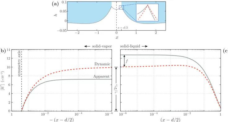
The differences between the localized-dissipation model and the full viscoelastic dynamic calculation can be interpreted in terms of true versus apparent contact angles. Figure 5(a) shows the profile in the approxima-tion of the localized-force model. The inset shows the violation of the Neumann balance: the red dashed line is the dynamic profile obtained from our viscoelastic the-ory. A more detailed view on the contact angles is given in fig. 5(b,c). Here we compare the dynamical slope (red dashed line) to that of the localized-force model (gray solid line), on both sides of the contact line atx=d/2. The two profiles have the same slope beyondx∼γs/Gh0.
However, differences appear at small distance near the contact line where viscoelastic dissipation plays a role. While the dynamic profiles are left-right symmetric, the localized-force model gives a symmetry breaking: the dif-ference in slope between the two approach at the contact line gives the magnitude off.
FIG. 5. (a) Resultant deformation in the localized-force model, obtained by superimposing two static profiles (d= 1/2, for α= 1/5 and αs = 1). The gray curve represents a resultant static profile. The red dashed curve shows the corresponding
dynamic wetting ridge that maintains equilibrium shape. (b), (c) Slope of the resultant deformation profiles (dynamic and static) measured away from the contact line atx=d/2 = 1/4 in both directions. The red dashed lines are the dynamic slopes, approaching γ/2γs at the contact line. The gray lines correspond to the localized-force model, showing an apparent contact
angle that differs by an amountf.
balance, due to a dissipative forcef. In reality the Neu-mann balance is restored at small distance, but the total dissipative force is indeed equal to f. At separations
d < γs/Gh0, however, the spatial distribution of
dissipa-tion has significant effects and the localized-force model gives rise to some (minor) quantitative errors.
IV. DROPS OF FINITE SIZE
We now show that interaction is dramatically changed when considering drops of finite sizeR, compared to the substrate thicknessh0. A fully consistent dynamical the-ory is challenging for finite-sized drops, since the two contact lines of a single drop are not expected to move at the same velocity. However, the previous section has shown that the localized-force model provides an excel-lent description of the interaction force, which becomes exact at separations d > γs/Gh0. We therefore follow
this approximation to quantify the inverted Cheerios ef-fect for finite sized drops.
A. Effect of substrate thickness
We assume that during interaction, radius of both the drops does not change and the liquid cap remains circular
(i.e. no significant dissipation occurs inside the liquid). The traction applied by a single drop on the substrate comprised of two localized forces pulling up at the contact lines and a uniform Laplace pressure pushing down inside the drop. The traction applied by a single drop of size
R, centered at the origin, is thus given by
Td(x) =γsinθeq[δ(x+R) +δ(x−R)]
−γsinθeq
R Θ(R− |x|),
(22)
expressed in dimensional form. Here Θ is the Heavi-side step function. The corresponding Fourier transform reads
e
Td(q) = 2γsinθeq
cos(qR)−sin(qR)
qR
. (23)
Considering two drops centered atx=−ℓ/2 andx=ℓ/2 respectively, with corresponding tractions ofTd(x+ℓ/2)
and Td(x−ℓ/2), the total traction induced by the two
drops reads, in Fourier space
e
T(q) =Ted(q)eiqℓ/2+Ted(q)e−iqℓ/2, (24)
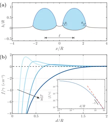
corre-FIG. 6. (a) Substrate deformation and liquid cap shape due to two interacting drops centered at x = ±5/4. The sep-aration distance between two neighboring contact lines is d/R = ℓ/R−2 = 1/2. (b) The interaction force vs dis-tance plot as the substrate thickness to drop radius ratio is increased (h0/R= 1/10,1/5,2/5,1). For thick substrates the interaction becomes predominantly attractive. Inset: Force vs distance plot on log scale for finite drops of an elastic half space. The red dashed line is the far-field asymptotic rep-resenting f ∼d−5
. The parameters used in this figure are γ/GR= 2/5, andγs/GR= 1/5. θeq for this case is found to
be 78.91◦.
sponding deformation profiles. A typical profile obtained from this traction is shown in fig. 6.
The problem is closed by determining the liquid con-tact angles at both the concon-tact lines (θi, θo)
self-consistently with the elastic deformation [20]. The inter-action is found from reestablishing a violated Neumann balance by a dissipative force (for details we refer to [16]). As such we determine the force-distance relation for vary-ing drop sizes. The results are shown in fig. 6(b), for var-ious drop sizesh0/R. Clearly, upon decreasing the drop size, or equivalently increasing the layer thickness, the interaction force becomes predominantly attractive. For a thin substrate, incompressibility leads to a sign change of the interaction force. As the substrate thickness is increased the profile minimum is moved away from the contact line. For an elastic half space, i.e. h0/R=∞, the deformation monotonically decays away from the contact line giving rise to a purely attractive interaction. The in-set of fig. 6(b) shows the interaction force for an elastic half space.
B. Far-field asymptotics on a thick substrate
When two drops are far away from each other, θi =
θo ≃ θeq and the liquid cap resembles its equilibrium
shape. In this limit, the drop-drop interaction is medi-ated purely by the elastic deformation. Here we calculate the large-dasymptotics of the interaction force. We fol-low a procedure similar to that proposed for elasticity-mediated interactions between cells [31, 32], where the cells are treated as external tractions. The total energy of the systemEtot then consists of the elastic strain
en-ergyEeℓplus a termEw originating from the work done
by the external traction. At fixed separation distance, the mechanical equilibrium of the free surface turns out to give Eeℓ = −12Ew (the factor 1/2 being a
conse-quence of the energy in linear elasticity). So, we can write Etot =Eeℓ+Ew =−Eeℓ [32]. Subsequently, the
interaction force between the droplets is computed as
f =−dEtot dd =
dEeℓ
dd . The task will thus be to evaluate
Eeℓfrom the traction induced by two drops.
In the absence of body forces, the elastic energy (per unit length) is written as
Eeℓ=
1 2
ˆ ∞
−∞
T(x)h(x)dx
= 1 2G
ˆ ∞
−∞
e
T(q)Te(−q)Ke(q)dq 2π.
(25)
Plugging in the traction applied by two drops given in eq. (24) into eq. (25) we find that there are two parts of the elastic energy: one is due to the work done by individual tractions (the self-energy of individual drops), and an interaction term (Eint) given by
Eint=
1
G
ˆ ∞
−∞
e
Td(q)Ted(−q)Ke(q) eiqℓ+ e−iqℓ
dq
4π. (26)
To obtain the far-field interaction energy (ℓ≫R), we now perform a multipole expansion of the tractionTd(x),
or equivalently a long-wave expansion of its Fourier trans-form. The quadrupolar traction of eq. (23) gives, after expansion
e
Td(q)≃
(−iq)2
2 Q2, (27)
were Q2 is the second moment of the traction and is given by,Q2 = ´−∞∞ Td(x)x2dx = 43γsinθeqR2. So, the
interaction energy in the far-field reads
Eint≃ 1
G
ˆ ∞
−∞ (iq)4
22 Q 2
2Ke(q) eiqℓ+ e−iqℓ
dq
4π
= Q 2 2 8G(K
′′′′(ℓ) +K′′′′(−ℓ)).
For drops on a finite thickness, the Green’s functionK(x) decays exponentially and again gives an exponential cut-off of the interaction at distances beyondh0.
A more interesting result is obtained for an infinitely thick substrate, formally corresponding to h0 ≫ℓ. The kernel for a half space is K(x) =−log2π|x|, which can e.g. be inferred from the large thickness limit of (5). Conse-quently, K′′′′(ℓ) =K′′′′(ℓ) = 3
πℓ4, so that the interaction
energy becomes
Eint= 4
3π
(γsinθeq)2
G R4
ℓ4. (29)
This is identical to the interaction energy between capil-lary quadrupoles [12, 33, 34], except for the prefactor that depends on elastocapillary length in the present case. We calculate the force of interaction byf = dEint
dℓ , giving
f γ =−
16 sin2θeq
3π
γ
GR R
ℓ
5
≃ −16 sin
2θ
eq
3π
γ
GR R
d
5
, (30)
where the result is collected in dimensionless groups. Here we replaced ℓ ≃ d, which is valid when the drop separation is large compared to R. The red dashed line in the inset of fig. 6(b) confirms the validity of the above asymptotic result, including the prefactor. Hence, in the limit of large thickness the attractive interaction force decays algebraically, as 1/d5, which is in stark contrast to the exponential decay observed for thin substrates.
It is instructive to compare eq. (29) with the inter-action energy for capillary quadrupoles formed by rigid anisotropic particles embedded in a fluid-fluid interface [5, 12]. In that case an undulated triple line is formed owing to contact line pinning [12] or to the change in cur-vature of the solid surface along the triple line [9, 35]. For capillary quadrupoles the far-field interaction energy is proportional toγH2
p(R/ℓ)4, whereHpis the amplitude of
the quadrupolar contact line distortion. Despite an iden-tical power-law dependence, the prefactors in eq. 29 and in the corresponding expression for capillary quadrupoles are different, reflecting a different physical origin. A cap-illary quadrupole is formed by four lobes located at an average distance R from the quadrupole center: two pos-itive meniscus displacements of amplitude Hp along one
symmetry axis of the particle, and two negative displace-ments along the perpendicular axis. The presence of a second particle changes the slope of equal sign meniscii along the center-to-center line, resulting in a net capillary attraction. The corresponding interaction force per unit length of contact line is proportional toγ(Hp/R)2(R/d)5,
to be compared with eq. 30. The non-dimensional ratio (Hp/R) is a geometric feature of the particle that
de-pends primarily on the particle shape and contact angle [5]. This ratio is independent of the particle size. On the contrary, the non-dimensional ratio GRγ does depend
on the particle size, as well as on the material-dependent scale γ/G. A differentiating feature is also that in the elastocapillary quadrupole the upward and downward distortions of the elastic surface are located along the line of interaction, thus forming a linear quadrupole. The identical power-law dependence for capillary and elasto-capillary quadrupoles is incidental. It is a consequence of the fact that the log function is the Green’s function for both the small-slope Young-Laplace equation of cap-illarity and the equation governing 2D linear elasticity.
V. DISCUSSION
Finally, let us turn to experiments of the inverted Cheerios effect. The results in fig. 1 already show a qualitative agreement between theory and experiment. A quantitative comparison in terms of “velocity vs dis-tance” is challenging, since the experimental motion fol-lows is due to a combination of drop-drop interaction and gravity – the latter was not taken into account in the dy-namical theory. However, gravity is easily substracted when representing the result as “force vs distance”, as was also done in [16]. The experimental data are re-produced in fig 7: On thick substrates the interaction is purely attractive (panel b), while a change in sign of the interaction force is observed on thin substrates (panel a). The two-dimensional model presented in this paper predicts a force per unit length f. Hence, to compare to experiment one needs to multiply the result with a proper length over which this interaction is dominant. The blue lines are obtained by choosing a length ofπR/6, i.e. a small fraction of the perimeter, giving a good agree-ment with experiagree-ment. In [16] we provided numerically a three-dimensional result, based on the same localized-force approach. The result is shown as the red lines in fig. 7 and is similar to the two-dimensional case. This good agreement with experiment shows that the elasto-capillary theory presented here provides an accurate de-scription of the physics. The similarity between the two-and three-dimensional models shows that the interaction is dominated by the regions where the contact lines are closest.
FIG. 7. Comparison between theory and experiment. The experimental data (black points) and 3D theory (red dashed lines) is reproduced from [16]. The drops have an average radius (R) of 700µm in both cases. The liquid (ethylene glycol) and the solid (PDMS) surface tensions areγ = 48 mN/m, andγs≃20 mN/m respectively. Shear modulus of the substrate isG= 280 Pa.
The blue lines are the interaction force obtained from 2D theory. (a) Attraction and repulsion on a substrate of thickness (h0) 40µm. (b) Purely attractive interaction between drops on a thick substrate (h0 = 8 mm). The adjustable length, multiplied with the 2D interaction force for comparison with the experiments isπR/6 for both the cases.
the ratio of substrate thickness to drop radius governs the nature of the interaction. In the other physically rel-evant limit of small drops on a very thick substrate, the interaction force is found to decay algebraically for large distances. We anticipate that the dissipation mediated interaction mechanism studied here to play a key role in collective dynamics of drops on soft surfaces [26, 36], and dynamics of soft, adhesive contacts.
Appendix
We evaluate the complex counterpart of the integrand in eq. (17) on a contourC, given by
α
‰
C
iq "
αsq2+ 1 e
K(q) #−1
eiqddq
2π. (A.1)
Hereq is the complex wave vector. The contourC
con-sists of a semicircle of radiusrcentered at the origin and a straight line connecting the ends of the semicircle. We evaluate the above integral using Residue theorem. As
r→ ∞, the integrand vanishes on the semicircle and the contour integral simplifies to eq. (17). For anyαsthe
in-tegrand of eq. A.1 has an infinite number of poles on the complex plane. The leading order behavior of the inte-gration is governed by the pole with smallest imaginary part (qpole) as other poles lead to much faster decay.
The substrate elastocapillary number αs dictates the
value ofqpole. Figure 8 shows that below a critical αs,
qpole is purely imaginary suggesting an purely
exponen-tial decay of the deformation. Beyond the critical αs,
qpole has a nonzero real and imaginary part giving rise
to oscillatory behavior of slope as predicted by Long et.
al [24]. Hence, the large distance approximation of slope
FIG. 8. Variation of qpole on the complex plane with the
elastocapillary numberαs. Below a criticalαs,qpoleis purely
imaginary and signifies an exponential decay.
is given by,
H−′ v≃2πi Res
"
αiq
αsq2+ e1
K(q) eiqd
2π
#
q=qpole
. (A.2)
This expression simplifies to eq. (18) in the main text.
ACKNOWLEDGMENTS
[1] D. Vella and L. Mahadevan, American Journal of Physics 73, 817 (2005), http://dx.doi.org/10.1119/1.1898523.
[2] D. Vella, Annual Review of Fluid Mechanics 47, 115 (2015), http://dx.doi.org/10.1146/annurev-fluid-010814-014627.
[3] P. A. Kralchevsky and K. Nagayama, Advances in Colloid and Interface Science85, 145 (2000).
[4] J. C. Loudet, A. M. Alsayed, J. Zhang, and A. G. Yodh, Phys. Rev. Lett.94, 018301 (2005).
[5] L. Botto, E. P. Lewandowski, M. Cavallaro, and K. J. Stebe, Soft Matter8, 9957 (2012).
[6] D. Ershov, J. Sprakel, J. Appel, M. A. Cohen Stuart, and J. van der Gucht, Proceedings of the National Academy of Sciences110, 9220 (2013).
[7] J. C. Loudet and B. Pouligny, The European Physical Journal E34, 76 (2011).
[8] N. Bowden, A. Terfort, J. Carbeck, and G. M. White-sides, Science276, 233 (1997).
[9] E. P. Lewandowski, M. Cavallaro, L. Botto, J. C. Bernate, V. Garbin, and K. J. Stebe, Langmuir 26, 15142 (2010).
[10] E. M. Furst, Proceedings of the National Academy of Sciences108, 20853 (2011).
[11] M. Cavallaro, M. A. Gharbi, D. A. Beller, S. ˇCopar, Z. Shi, T. Baumgart, S. Yang, R. D. Kamien, and K. J. Stebe, Proceedings of the National Academy of Sciences 110, 18804 (2013).
[12] D. Stamou, C. Duschl, and D. Johannsmann, Phys. Rev. E62, 5263 (2000).
[13] A. Chakrabarti, L. Ryan, M. K. Chaudhury, and L. Ma-hadevan, EPL (Europhysics Letters)112, 54001 (2015).
[14] A. Chakrabarti and M. K. Chaudhury,
Lang-muir 30, 4684 (2014), pMID: 24702043,
http://dx.doi.org/10.1021/la5007988.
[15] A. Chakrabarti and M. K. Chaudhury, Langmuir 29, 15543 (2013).
[16] S. Karpitschka, A. Pandey, L. A. Lubbers, J. H. Weijs, L. Botto, S. Das, B. Andreotti, and J. H. Snoeijer, Pro-ceedings of the National Academy of Sciences113, 7403 (2016).
[17] A. D¨orr, S. Hardt, H. Masoud, and H. A. Stone,Journal of Fluid Mechanics, 790, 607 (2016).
[18] A. Carre, J.-C. Gastel, and M. E. R. Shanahan, Nature
379, 432 (1996).
[19] A. Marchand, S. Das, J. H. Snoeijer, and B. Andreotti, Phys. Rev. Lett.109, 236101 (2012).
[20] L. A. Lubbers, J. H. Weijs, L. Botto, S. Das, B. An-dreotti, and J. H. Snoeijer,Journal of Fluid Mechanics, 747(2014), DOI: 10.1017/jfm.2014.152.
[21] S. J. Park, B. M. Weon, J. S. Lee, J. Lee, J. Kim, and J. H. Je, Nature Communications5, 4369 EP (2014).
[22] S. Karpitschka, S. Das, M. van Gorcum, H. Perrin, B. An-dreotti, and J. H. Snoeijer, Nature Communications6, 7891 EP (2015).
[23] J. Ferry, Viscoelastic properties of polymers (Wiley, 1961).
[24] D. Long, A. Ajdari, and L. Leibler, Langmuir12, 5221 (1996).
[25] E. R. Jerison, Y. Xu, L. A. Wilen, and E. R. Dufresne, Phys. Rev. Lett.106, 186103 (2011).
[26] R. W. Style, Y. Che, S. J. Park, B. M. Weon, J. H. Je, C. Hyland, G. K. German, M. P. Power, L. A. Wilen, J. S. Wettlaufer, and E. R. Dufresne, Proceedings of the National Academy of Sciences110, 12541 (2013).
[27] R. W. Style, R. Boltyanskiy, Y. Che, J. S. Wettlaufer, L. A. Wilen, and E. R. Dufresne, Phys. Rev. Lett.110, 066103 (2013).
[28] H. H. Winter and F. Chambon, Journal of Rheology30, 367 (1986).
[29] J. C. Scanlan and H. H. Winter, Macromolecules24, 47 (1991).
[30] F. Chambon and H. H. Winter, J. Rheol.31, 683 (1987).
[31] U. S. Schwarz and S. A. Safran, Phys. Rev. Lett. 88, 048102 (2002).
[32] I. B. Bischofs, S. A. Safran, and U. S. Schwarz, Phys. Rev. E69, 021911 (2004).
[33] K. D. Danov, P. A. Kralchevsky, B. N. Naydenov, and G. Brenn, Journal of Colloid and Interface Science287, 121 (2005).
[34] K. D. Danov and P. A. Kralchevsky, Advances in Colloid and Interface Science154, 91 (2010).
[35] J. C. Loudet, A. G. Yodh, and B. Pouligny, Phys. Rev. Lett.97, 018304 (2006).

![FIG. 7. Comparison between theory and experiment. The experimental data (black points) and 3D theory (red dashed lines) is reproduced from [16]](https://thumb-us.123doks.com/thumbv2/123dok_us/8175117.2167207/10.918.93.836.75.310/comparison-theory-experiment-experimental-points-theory-dashed-reproduced.webp)
