Evolution in the context of the environment

EVOLUTION IN THE CONTEXT OF THE ENVIRONMENT

AMANDA JOAN CHUNCO

A dissertation submitted to the faculty of the University of North Carolina at Chapel Hill in partial fulfillment of the requirements for the degree of Doctor of Philosophy in the Department of Biology.

Chapel Hill 2009

Approved by:

© 2009

ABSTRACT

AMANDA JOAN CHUNCO: Evolution in the Context of the Environment (Under the direction of Maria R. Servedio and Karin S. Pfennig)

Ecology can strongly influence evolution. To fully understand the evolutionary history of a species, it is essential to consider evolution within the context of the environment. Here, I explore how the environment produces different evolutionary patterns between populations and species, while considering how evolution in turn affects ecological patterns of distribution and population viability.

Within a single population, the environment can affect whether polymorphisms are maintained or lost. Using a population genetic model, I show how natural and sexual selection can result in the maintenance of male color polymorphisms (MCPs) in a single population. Specifically, I find that microhabitat heterogeneity can lead to MCP

maintenance despite asymmetries in the strengths of natural and sexual selection and in microhabitat proportions. Also, while sexual selection alone is often sufficient for

polymorphism maintenance, natural selection alone results in polymorphisms under only unrealistic conditions.

species distribution and community composition and macroevolutionary processes including speciation and species level selection.

Finally, I examined how the environment can influence range dynamics and species interactions in two spadefoot toad species. First, I used museum specimens to describe recent changes in species distribution. I found that these species have

ACKNOWLEDGEMENTS

This work was not created in isolation, but reflects a great deal of support, of many different kinds, from a community of friends and colleagues. I first and foremost want to thank my committee. Karin Pfennig provided the academic freedom to pursue my own interests, while teaching me a great deal about using research to tell a compelling and broadly interesting story. Maria Servedio has been not only a great collaborator and teacher, but also a friend and valuable resource for advice on both career and family issues. The rest of my committee, including David Pfennig, Joel Kingsolver, and Aaron Moody, has been instrumental in helping me reach my professional goals by providing both a thoughtful critique of my work and broad training that will give me the flexibility to teach, do research, or both after I graduate.

My labmates, half labmates, office mates and grad school friends were a great source of research advice, feedback on talks and manuscripts, and more than anything else, emotional support and lots of fun. Ryan Martin, Amber Rice, Martin Ferris, Sarah Joseph, Jennifer Knies, Christy Violin, Sarah Diamond, Helen Ivarsson, Greg Ragland, and Cris Ledón-Rettig have been and continue to be amazing friends and the best part of grad school.

My family, both those related by blood and by marriage, have always been there for me when I needed them, and I feel incredibly lucky to have their love and support.

TABLE OF CONTENTS

Page List of Tables………..………..…viii List of Figures…………...……….………….………ix Chapter I Introduction ………..………..………1 Chapter II Microhabitat variation and sexual selection can maintain male

color polymorphisms ..………....………….…...…...6 Chapter III Extinction via adaptive mate choice: ecological and evolutionary

implications………..………...………..44 Chapter IV Comparing ranges: using historic data to test hypotheses

about range expansion ………...………...66 Chapter V Where the twain shall meet: developing models for understanding

LIST OF TABLES

Table

2.1 Mating Table – Within habitat mate choice...37 2.2 Stability regions for asymmetrical parameter combinations…...…………..…….…38 2.3 Mating Table – Across habitat mate choice………..…………..39 5.1 Variables used in all niche models ………...119 5.2 The relative contribution of abiotic variables contributing at least

5% to the predictive model across the range at a 5km resolution for both

S. bombifrons and S. multiplicata ………...……….……..120 5.3 The relative contribution of abiotic variables contributing at least

5% to the predictive model within the region of co-occurrence at a 1km

LIST OF FIGURES

Figure

2.1 Regions of stability of the polymorphic equilibrium for three values of hyassuming natural and sexual selection are symmetrical for blue and

yellow morphs (sb = sy and ab = ay = a)……...40 2.2a The region of stability of the polymorphic equilibrium when female

preferences are symmetrical and natural selection is removed from the

model (ab= ay = a, sb= sy= 0)………...41 2.2b The frequency of the blue morph at different strengths of female

preference (a) and habitat frequency (hy) when natural selection is removed

(sb= sy= 0) and sexual selection is symmetrical between habitats (ab = ay = a)...42 2.2c The strength of female preference that will maintain a color

polymorphism when natural selection is not acting (sb= sy= 0) for three

different ratios of habitat frequency………...………..…………..43 4.1 Museum collection records for both S. bombifrons and S. multiplicata,

plotted by year of collection ………...88 4.2 Collection records over time for both S. multiplicata and S. bombifrons……...89 4.3 Zoomed in map of San Simon region………..………...…90 4.4 The number of unique collection sites for both S. bombifrons and

S. multiplicata over time within the San Simon population………..91 4.5 The cumulative log transformed (log10) number of unique collection

sites for both S. bombifrons and S. multiplicata over time within the San

Simon population………...92 5.1 The predicted distribution of S. bombifrons (a) and S. multiplicata

(b) across the range using environmental and point data at a 5 km resolution………....122 5.2 The predicted distribution of S. bombifrons (a) and S. multiplicata

(b) within the region of predicted co-occurrence given by the model of the

entire range using environmental and point data at a 1 km resolution………...123 5.3 Areas of predicted co-occurrence between S. multiplicata and

S. bombifrons using data at a 5km resolution. Both the total range (a)

5.4 The predicted distribution of S. bombifrons, S. multiplicata, and both species using a 1km resolution, within the area predicted to have both

species as identified in the range model in Fig 3……….…. ..125 5.5 All test ponds mapped by altitude in and around the San Simon valley

(the specific region is shown as a box on the insert map) (a), and a subset

of the ponds showing the specific altitudinal gradient (b)………...126 5.6 The location of test ponds mapped on the prediction of best habitat for

S. bombifrons (a) and S. multiplicata (b)……….127 5.7 Test ponds mapped over the predicted areas co-occurrence in

southeastern Arizona (a) and specifically around an area where mixed

species ponds are common (b)………..…...128

CHAPTER I

INTRODUCTION

Understanding how the environment influences the evolution of a species is a

fundamental goal of evolutionary ecology. The biotic and abiotic elements in any given

environment define the ecology of the species that live there, and these elements play a

major role in shaping the evolution of these species. Over short timescales, the

environment can influence the distribution and abundance of a species. Over longer

timescales, the distribution and abundance of a single species will affect other species in

the community. These species interactions can result in potentially novel biotic

environmental factors that will in turn have consequences for the evolution of the

interacting species. Thus, considering the environment is essential to fully understanding

both the evolutionary history and the evolutionary trajectory of a species.

Determining what specific effects the environment may have on populations is,

however, a challenging task because the environment is rarely constant. Indeed, the

spatial and temporal heterogeneity both within a habitat (i.e. microhabitat variation) and

between habitats will strongly affect the selection pressures facing organisms within that

environment. Habitat heterogeneity can influence evolution and ecology at multiple

scales, from the existence of polymorphisms within a single population (Fuller et al.

2005), to more complex interactions between species across wide geographic ranges

In this thesis, I consider the ecological and evolutionary consequences of

environmental heterogeneity at multiple biological scales (both within and between

species) as well as at multiple geographic scales (from microhabitats to species ranges).

In doing so, my goal is to use multiple approaches to address questions about how the

environment produces different evolutionary and ecological patterns between both

populations and species.

Within even a single population, habitat variation can influence the evolutionary

trajectory of that population. Indeed, spatial and temporal variation is an important

explanation for the existence of phenotypic polymorphisms (Skúlason and Smith 1995).

One example of phenotypic polymorphism is male color polymorphism (MCP). While

male color polymorphisms are ubiquitous in nature (Barlow 1973; Anderson 1994;

Hoffman and Blouin 2000), the maintenance of these polymorphisms is not yet fully

understood. In Chapter 2, I use a population genetic model to investigate the specific

environmental conditions that promote the maintenance of male color polymorphisms. In

the model, I consider a single population with two male color morphs. This population is

found in an area with two microhabitats. In one microhabitat, one morph is more

conspicuous, while in the other microhabitat, the second morph is more conspicuous.

This mimics a habitat that varies bimodally, such as aquatic habitats during morning vs.

midday sunlight. Using this simple, but biologically plausible model, I can evaluate how

habitat heterogeneity contributes to either polymorphism loss or maintenance. The results

of this model are reprinted here with permission from the journal Evolution (Chunco et

Across populations, environmental heterogeneity can lead to divergent

evolutionary paths, and may potentially lead to speciation or even differential extinction

risk. In Chapter 3, I consider how environmental difference between populations can

affect female mate choice, specifically in cases where individual fitness is improved at

the cost of population level fitness (i.e. “Darwinian extinction”, Houle & Kondrashov

2002; Webb 2003). As female mate choice is often dependent on the environment,

environmental difference can result in divergent female mate choice preferences. For

example, in high predation environments, females may alter their preferences in the

presence of predators, while those from low predation environments do not (e.g. Godin &

Briggs 1996). I suggest that when females in different habitats must make different

tradeoffs in mate choice, populations can diverge, potentially resulting in differences in

average fecundity and potentially population viability.

Across the range of an entire species, the distribution and abundance of a species

will be determined by abiotic and biotic factors in the environment. Studying this

phenomenon is becoming increasingly important as anthropogenic change is affecting the

environments in which species live and interact, potentially resulting in entirely novel

species interactions (e.g. Williams and Jackson 2007). In Chapter 4, I consider the effects

of land-use change on the distribution and abundance of two species of spadefoot toads in

the southwestern United States. Changes in agriculture, particularly cattle ranching, may

have influenced these species because reproduction in both species is tied to ephemeral

ponds that are often modified by ranchers. To capture historic patterns of when each

species first arrived in the southwest, and to characterize how these species saturated this

important source for historic data (Graham 2004), but I argue here that more systematic

efforts at data collection and storage will be necessary to document the increasing effects

of anthropogenic change.

Finally, at the level of multi-species interactions, the environment can influence

whether species coexistence or competitive exclusion will occur in a given habitat. In

Chapter 5, I use ecological niche modeling to look at the role of various abiotic and biotic

factors in shaping distributions across the ranges of two species of spadefoot toads.

Creating a model of predicted distributions of both species based on only abiotic factors

provides a null distribution against which the effects of various biotic factors can then be

tested. At the same time this work can be used to show where both are most likely to

co-occur, providing targeted areas for future field studies.

Through this dissertation work, I aim to show some of the ways through which

habitat variation can influence both evolutionary and ecological patterns, from the scale

REFERENCES

Anderson, M. 1994. Sexual selection. Princeton University Press, Princeton.

Barlow, G. W. 1973. Competition between color morphs of the polychromatic midas cichlid Cichlosoma citrinellum. Science 179:806-807.

Chunco, A. J., J. S. McKinnon, and M. R. Servedio. 2007. Microhabitat variation and sexual selection can maintain male color polymorphisms. Evolution 61: 2504-2515.

Fuller, R. C., K. L. Carleton, J. M. Fadool, T. C. Spady, and J. Travis. 2005. Genetic and environmental variation in the visual properties of bluefin killifish Lucania goodei. J. Evol. Biol. 18:516-523.

Gaston, K. J. 2003. The structure and dynamics of geographic ranges. Oxford University Press.

Godin, J.-G. & Briggs, S. E. 1996 Female mate choice under predation risk in the guppy.

Anim. Behav.51, 117-130.

Graham, C. H., S. Ferrier, F. Huettman, C. Moritz, and T. Peterson. 2004. New

developments in museum-based informatics and applications in biodiversity analysis. Tree 19: 497-503.

Hoffman, E. A. and M. S. Blouin. 2000. A review of colour and pattern polymorphisms in anurans. Biol. J. Linn. Soc. 70:633-665.

Houle, D. & Kondrashov, A. S. 2002 Coevolution of costly mate choice and condition- dependent display of good genes. Proc. R. Soc. B269, 97-104.

Skúlason, S. and T. B. Smith. 1995. Resource polymorphisms in vertebrates. Trends in Ecol. Evol. 10: 366-370.

Webb, C. 2003 A complete classification of Darwinian extinction in ecological interactions. Am. Nat. 161, 181-205.

CHAPTER II

MICROHABITAT VARIATION AND SEXUAL SELECTION CAN MAINTAIN MALE COLOR POLYMORPHISMS

Abstract– Male color polymorphism may be an important precursor to sympatric

speciation by sexual selection, but the processes maintaining such polymorphisms are not

well understood. Here, we develop a formal model of the hypothesis that male color

polymorphisms may be maintained by variation in the sensory environment resulting in

microhabitat specific selection pressures. We analyze the evolution of two male color

morphs when color perception (by females and predators) is dependent on the

microhabitat in which natural and sexual selection occur. We find that an environment of

heterogeneous microhabitats can lead to the maintenance of color polymorphism despite

asymmetries in the strengths of natural and sexual selection and in microhabitat

proportions. We show that sexual selection alone is sufficient for polymorphism

maintenance over a wide range of parameter space, even when female preferences are

weak. Polymorphisms can also be maintained by natural selection acting alone, but the

conditions for polymorphism maintenance by natural selection will usually be unrealistic

for the case of microhabitat variation. Microhabitat variation and sexual selection for

conspicuous males may thus provide a situation particularly favorable to the maintenance

of male color polymorphisms. These results are important both because of the general

in natural populations and because such variation is an important prerequisite for

sympatric speciation.

Key Words – sympatric speciation, predation, habitat heterogeneity, female choice, model

INTRODUCTION

Polychromatism is widespread in nature (Barlow 1973; Anderson 1994; Hoffman

and Blouin 2000; Gray and McKinnon 2006, 2007) and has long been central to studying

the maintenance of variation within natural populations of animals (Ford 1965; Roulin

2004). Male color polymorphisms (MCPs), a type of polychromatism in which males

within the same population exhibit different, discrete color morphs, is of particular

interest both because of the role sexual selection may play in the evolution of such

polymorphisms (Eakley and Houde 2004; Seehausen and Schluter 2004) and because

MCPs may play an important role in sympatric speciation (Seehausen et al. 1999;

Allender et al. 2003).

Several hypotheses have been proposed to explain the maintenance of MCPs.

These include negative frequency dependent male-male competition (in cichlids,

Seehausen and Schluter 2004), negative frequency dependent predation on male color

morphs (in guppies, Olendorf et al. 2006) a balance between female preference and male

aggression (in swordtails, Xiphophorus pygmaeus, Kingston et al. 2003), female

preferences for unfamiliar or novel males (Hughes et al. 1999; Eakley and Houde 2004;

Kokko et al. 2007), and spatial and temporal habitat heterogeneity (Fuller et al. 2005). As

male color is potentially selected on by both predators and females, both types of

predation often favors inconspicuous traits, while sexual selection often favors

conspicuousness (Endler 1980; Anderson 1994; Zuk and Kolluru 1998).

Given that signal perception is highly habitat dependent (Endler 1980; Bradbury

and Vehrencamp 1998; Chiao et al. 2000), it is impossible to interpret the signal outside

the context of the environment. Color perception depends on the properties of the signal,

the light under which the signal is perceived, the background against which it is viewed,

the medium through which the signal is sent (i.e. air or water), and the sensory

capabilities of the receiver (Endler 1991; Chiao et al. 2000; Endler and Mielke 2005).

Therefore, if an environment is heterogeneous in substrate type, light intensity, or other

factors that influence signal perception, the potential exists for several different color

morphs to persist, as each morph will represent the optimal balance between natural and

sexual selection within a given visual microhabitat (Gamble et al. 2003). Indeed,

empirical evidence that habitat variation affects signal conspicuousness and the evolution

of male signals has now been obtained for several sensory systems from diverse taxa

including birds, lizards, frogs, insects, and fish (for a review, see Boughman 2002).

Although empirical evidence suggests a role for fine scale habitat variation in the

maintenance of MCPs, a formal theoretical analysis of how differential selection between

microhabitats may lead to the maintenance of male color polymorphisms has not

previously been developed. Here we present a population genetic model that looks at the

conditions under which habitat heterogeneity in qualities affecting color perception will

lead to the existence of a stable male color polymorphism. In so doing, we answer three

specific questions about the likelihood of this mechanism maintaining a polymorphism in

selection alone? 2) How robust are the conditions for MCP maintenance to asymmetries

in habitat frequencies and selection strengths? and 3) How does changing the biological

assumptions of the conditions under which selection occurs, for both natural and sexual

selection, influence the outcome of the model? Although we focus throughout on MCP’s

as our ‘case study’, our goal is to develop a relatively general model of how

environmental variation might contribute to the maintenance of variation in signals. For

this reason, we keep our model of signal conspicuousness relatively simple and general.

THE MODEL

In this haploid model, we consider a population of sexually dimorphic animals.

Males are polymorphic for color with two distinct morphs. For convenience, we refer to

them here as blue (occurring with frequency ) and yellow (occurring with

frequency ). These color patterns are common in fish MCPs (e.g. Seehausen and

Schluter 2004; Gray and McKinnon 2006) and are also seen in lizards (e.g. Sinervo and

Lively 1996). A great deal of work has been done on the genetic basis of blue and yellow

color polymorphisms, and in several of these systems, color expression is controlled in

large part by a single locus with multiple alleles (in swordtails, Xiphophorus pygmaeus,

Baer et al. 1995; in killifish, Lucania goodei, Fuller and Travis 2004; in side-blotched

lizards, Uta stansburiana, Sinervo and Zamudio 2001). Therefore, we modeled color as

being controlled by a single locus with two alleles. We assume that females are

monomorphic for color and that color is entirely genetically controlled in both sexes.

Although color does not indicate genetic or phenotypic quality, it does affect fitness in

b p

that males that are more conspicuous within their environment are both more vulnerable

to predation and more likely to be chosen by females.

The habitat in which natural and sexual selection occurs is divided into

microhabitats that differ in physical properties that influence color perception, such as

light intensity, light spectrum, and/or substrate color and pattern. Because of these

differences in visual properties, each microhabitat provides a functionally different

setting within which male color is perceived by females and by predators. Environmental

heterogeneity encountered by an individual is not the result of migration; rather, variable

visual backgrounds within the general environment result from fine-scaled spatial or

temporal differences (e.g. Gamble et al. 2003).

We specifically consider an environment with two microhabitats. The blue male

color morph is more conspicuous than the yellow male morph in habitat Hb (occurring

with frequency hb), while in habitat Hy (occurring with frequency hy = 1-hb), the reverse

is true. Both sexes move freely and randomly between habitats (neither males nor females

actively choose a habitat) so that each sex has a probability of being in each microhabitat

according to relative habitat area.

The life cycle begins with the zygote stage. Natural selection follows birth and

acts exclusively on males. The more conspicuous morph in each microhabitat suffers a

greater loss from predation. Specifically, sb represents the selection coefficient against

blue males in habitat Hb, while sy is the selection coefficient against yellow males in

habitat Hy. Because habitat varies on a small (microhabitat) scale, we model natural

selection as occurring across habitats that organisms can freely move between (see

selection (superscript “ns”) isw_bns h_b





the absolute fitness of the yellow morph islikewise . The frequency of the

blue morph ( ) after males undergo natural selection ( ), is given by equation 1:

b b ns

b h s

w 1

y y ns

y h s

w 1

* b p b p pb

* _ pbwb ns

pbwb ns

pywy

ns. (1)

Since females do not express the color alleles, the frequency of the blue allele carried by

females at this stage of the life cycle remainspb.

After natural selection, mating (sexual selection) occurs. We assume a

polygynous system where females have equal mating success (e.g. Kirkpatrick 1982) and

males provide no resources to females other than their genetic contribution. The sole

advantage males of each color possess over differently colored competitors is their

microhabitat-dependent conspicuousness. This advantage is represented by a factor ai

(where i = b or y depending on the microhabitat that the female is in), where females are

ai times more likely to mate with a more conspicuous morph than a less conspicuous

morph if they encounter one of each.For now, we assume that females choose between

blue and yellow males within their current microhabitat. That is, females are either in

habitat Hb or Hy when mating decisions are made, and they can only view one

background at a time. Mating success of each male morph is thus determined separately

within each habitat (see Levene 1953).

number in Table 1) and j represents male type in each habitat (i.e. column number in

Table 1). The frequency of the blue color allele in the following generation ( ) is

shown by equation 2:

) 1 (t

p_b 42 31 24 22 13 11 2 1 2 1 2 1 2 1 ) 1

(t M M M M M M

p_b        . (2)

The final recursion can be obtained by substituting the appropriate values of the cells of

Table 1 into equation (2). Equilibrium frequencies were found by setting the offspring

frequencies at time t equal to the frequencies at time t+1 and solving the resulting

recursion equation.

RESULTS

Three equilibria result from this model. Two of the equilibria represent loss ( =

0) and fixation ( = 1) of the blue color morph. The third equilibrium is polymorphic.

The best way to understand the polymorphic equilibrium from the full model is to first

present the equilibrium under sexual selection alone (with no natural selection, sb = sy =

0). We are interested in the polymorphic equilibrium frequency of the blue morph,

b pˆ

ˆ ˆ

p _b

p b, so

we write the relative fitness of blue males, due to sexual selection alone (superscript

“ss”), as in the habitat where blue is conspicuous (Hb) and asw in

the habitat where yellow is conspicuous (Hy ) (the relative fitness of yellow males in

habitat Hy must also be rescaled throughout the results below to 1 instead of ay, changing b

a ss

Hb b

the normalization factor v in the mating table to wb,Hy ss

pb py). We can then express the

polymorphic equilibrium, due to sexual selection alone, as

) 1 ) 1 ( _,   Hy ss Hy b w )( 1 ( ) 1 ( ˆ , , ,      _ss b ss Hb b y ss Hb b b b w w h w h

p . (3)

The term is a measure of the selection coefficient favoring the blue morph due

to sexual selection in habitat Hb (this term will be positive since ab>1), while

represents the parallel selection coefficient against the blue morph in habitat Hy (this term

will be negative since ay>1). Equation (3) therefore shows that the polymorphic

equilibrium frequency of the blue allele due to sexual selection alone is a balance

between the frequency of habitat Hb times the selection coefficient favoring blue in that

habitat, and the frequency of habitat Hy times the selection coefficient against blue in that

habitat, scaled by the product of the selection coefficients (the minus sign in front of

equation (3) can be thought of as correcting for the negative selection coefficient in the

denominator).

) 1 ( ss_, 

Hb b w

) 1 ( ss_, 

Hy b w

To look at the equilibrium under the full model, we can simply replace the

fitnesses of the blue morph in equation (3) with ones that represent the action of both

natural and sexual selection (superscript “tot”). Therefore,

) 1 )( 1 ( ) 1 ( ) 1 ( ˆ , , , ,        _tot Hy b tot Hb b tot Hy b y tot Hb b b b w w w h w h

where tot _b and , and where

Hb

b A

w _,  w_btot_,Hy 1/A_y

ns y ns b b b w w a

A  and _ns

b ns y y y w w a

A  .

Ai is therefore equal to the strength of female preference, ai, for a color morph when it is

conspicuous, multiplied by the ratio of the fitnesses due to natural selection of the

conspicuous to the inconspicuous morph.

Stabilities of the equilibria were determined using a linear stability analysis. The

equilibrium p ˆ _b = 1 (that is, the fixation of the blue morph) will be unstable when

1 1 2 1 , ,

1 

         _tot Hy b y tot Hb b b p w h w h

 (5)

and the equilibrium p ˆ _b=0 (that is, the loss of the blue morph) will be unstable when



2 1

, ,

0    

tot Hy b y tot Hb b b

p h w h w





The eigenvalue p1 consists of terms describing the contributions by females and males to

increases in the frequency of the yellow morph, which is the potentially invading morph

when blue is fixed (i.e. p ˆ _b = 1), as follows. The factor of ½ is present because there are

contribution from females is 1. The following two terms, hb/ and hy/ represent

contributions from males in habitat Hb and males in habitat Hy respectively, scaled by the

relative fitnesses of the yellow morphs (the reciprocal of the fitnesses of the blue morph)

in each respective habitat. Likewise, the eigenvalue p0 consists of contributions by

females and males to the spread of the blue morph, the potentially invading morph when

the yellow morph is fixed (i.e. = 0), where and represent

contributions from males in each habitat scaled by the relative fitness in that habitat of

the blue morph.

tot Hb b w _, tot Hy b yw h _, tot Hy b w_, y p ˆ

p _b h_bw_btot_,Hb

Note that our solutions to this point elaborate upon the findings of Gliddon and

Strobeck (1975). Using our equation (4), we can write an equation for (where

,



b

y p

p 1 )

































p 1

4 4 y y y w w   1 1 y p h

 . (7)

This is equivalent to equation (1) in Gliddon and Strobeck (1975) when wy1 = 1/ , wy2

= 1, wy3 = 1/ , and wy4 = 1 correspond to the fitnesses of the yellow morph in males

in habitats Hb (for wy1) and Hy (for wy3) and females in habitats Hb (for wy2) and Hy (for wy4). Equation (7) contains a factor of ½ to account for the fact that sexual selection is

treated separately in each sex. Gliddon and Strobeck’s (1975) stability conditions (2) and

The polymorphic equilibrium will be stable when both conditions(5) and (6)

hold. If we make the appropriate substitutions for the w terms, we can see that

condition (5) is more likely to hold (the equilibrium

b tot

ˆ

p b = 1 is more likely to be unstable

and yellow is more likely to invade) with lower sexual selection favoring the blue morph

(ab), higher sexual selection favoring the yellow morph (ay), and higher fitness due to

natural selection of the yellow versus blue morph (sy < sb). The opposite conditions will

tend to promote instability of thep ˆ _b = 0 equilibrium and therefore the invasion of the blue

morph into a population of yellow individuals. When the appropriate balance is reached

in the strength of the natural and sexual selection parameters, given a specific ratio of the

habitats to one another, the polymorphic equilibrium will be maintained.

Although equation (4) and the conditions that follow from equations (5) and (6)

present analytical solutions to the model and an intuitive feel for the effects of the

parameters, we examine several cases graphically and numerically in order to illustrate

the conditions for stability in an easily interpretable manner. This is done using the

analytical results, not by separate simulations.

To illustrate the results when both natural and sexual selection are acting, we

began with the assumption that the strengths of natural selection and sexual selection are

symmetrical for blue and yellow morphs (sb = sy and ab = ay). Under these assumptions,

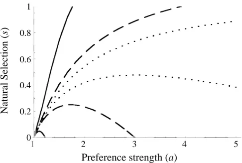
we find that the polymorphic equilibrium is stable under a broad range of conditions (Fig.

1). The values of preference and selection that result in a stable polymorphism are most

restricted when the habitats are highly skewed, but are more permissive as habitats

become more symmetrical. When habitats are exactly symmetrical (hb = hy = .5) in

regardless of the values of selection and preference. Again, however, even highly skewed

habitats can lead to a stable polymorphism with strong female preferences.

To illustrate the results when natural selection, sexual selection, and habitat

frequency deviated from symmetry, we found the eigenvalue at each of the three

equilibria (0, 1, and the polymorphic equilibrium; for the latter see (5) and (6)), solved for

ay, and then substituted specific values of sb, sy, hb, hy and ab into the resulting expression.

This allowed us to see what range of asymmetry in sexual selection strengths is

permissible to maintain the polymorphic equilibrium, given a set of parameter values. In

doing these tests, we evaluated a wide range of values for natural selection, sexual

selection, and habitat frequencies (s: 0.01-0.99; ab: 0-infinity; h: 0.01-0.99) for 60 unique

combinations of parameters. Representative examples of the outcomes of different

selection scenarios are presented in Table 2. We found that the polymorphic equilibrium

was generally stable over a range of parameter values (Table 2), however, when the

starting parameters were highly asymmetric, the range of parameter space leading to a

stable polymorphism could be quite restricted.

Finally, we evaluated a scenario where the morph favored by females also

suffered lower predation than the less favored morph (sb and sy < 0). This could result if

females favored more cryptic morphs. In this case, a stable polymorphism was again

possible, although the conditions resulting in a stable polymorphism show slight

numerical differences from cases with comparable selection strengths where female

preferences and natural selection favored different morphs (Table 2).

It is also illustrative to examine the effects of natural and sexual selection alone in

In this case, predators act indiscriminately, while females still preferentially choose

conspicuous males. Our polymorphic equilibrium for this scenario is shown in equation

(3), and the conditions for stability can be seen by setting sb = sy = 0 in the eigenvalues

(5) and (6) above, which yields a stable polymorphic equilibrium when

1 1

2 1

1 

      

 _{y y}

b b

p a h

a h

 and 1 1

2 1

0 

         y y b b p a h a h  .

Again, we can see that a stable polymorphism will be likely when a balance is struck

between the strengths of sexual selection and the habitat frequencies.

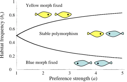
Under these conditions, female preference is often sufficient to maintain a

polymorphism. When preferences are symmetrical between habitats (ab = ay), even slight

female preference (i.e. a = 1.01) will maintain a polymorphism, although this requires

that habitat frequencies are also close to symmetrical (hb ≈ hy). As the strength of a

symmetrical female preference increases, a polymorphism will be maintained under

increasingly wide degrees of habitat asymmetry (Fig. 2a). The specific frequency of the

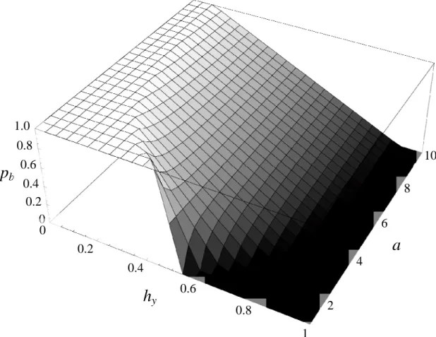
blue morph under different conditions of habitat frequency and strength of preference is

seen in Figure 2b. When we do not assume symmetry between female preference in each

habitat (abay), we find that a stable polymorphism is maintained under the widest range

of frequencies when habitats are close to symmetrical, with increasing strength of

preferences needed to maintain a polymorphism as habitat becomes increasingly skewed

(Fig. 2c). Additionally, when habitat frequencies are symmetrical, a polymorphism is

frequencies increases, a corresponding skew in preference strength (with stronger

preferences for the morph favored in the rarer habitat) is required to maintain a

polymorphism. Even under highly skewed conditions, however, a polymorphism will

occur if the strength of preference for the conspicuous morph in the rarer habitat is strong

enough.

We next looked at the outcome of natural selection alone (modeled here as

occurring across habitats, as described above) by removing the effects of sexual selection

(sb, sy > 0; ab = ay = 1). In this scenario, predators preferentially prey upon conspicuous

morphs, while females mate randomly. In this case, a polymorphism resulted only when

there were exactly symmetrical parameters between habitats (sb = sy, hb = hy) or when

selection and habitat area are exactly balanced. Any deviation from these conditions leads

to the fixation of either the blue or the yellow morph. These conditions of complete

symmetry are highly unrealistic and unlikely to occur in nature. This result is

unsurprising because several authors have demonstrated the difficulty of maintaining a

polymorphism when selection occurs across habitats, as we have modeled natural

selection here (eg. Dempster 1955; Christiansen 1975; Karlin and Campbell 1981; de

Meeûs et al. 1993).

ALTERNATIVE ASSUMPTIONS

In the model above, we consider the maintenance of a color polymorphism when

natural selection is assumed to occur across habitats (males of both morphs move

between habitats), whereas sexual selection occurs within habitats (females choose

when she is ready to mate). To confirm the effects of these assumptions on the outcome

of the model, we also examined the outcome of selection when we considered alternative

assumptions. That is, we modeled natural selection as occurring within one habitat (males

remain in one microhabitat throughout the period of natural selection and potentially

subsequent reproduction and predators stay within a habitat at least for each prey

selection event) and we modeled sexual selection occurring across habitats (females

examine males in both habitats before they choose a mate). In the discussion below, we

describe when these alternative assumptions may be appropriate.

To look at natural selection occurring within habitats, we use the notation ,

where i is b or y, to denote fitness of the blue and yellow morphs. Here, in habitat Hb, the

fitness of the blue morph is and the fitness of the yellow morph is .

In habitat Hy, where the yellow morph is conspicuous, the fitness of the blue morph is

and the fitness of the yellow morph is . After natural selection, the

frequency of the blue morph in microhabitat i is now

ns i w , ns Hb y b ns Hb b s

w_, 1 w 1

1

,  ns

Hy b

w w_yns_,Hy 1s_y

ns Hi y y ns Hi b b ns Hi b b Hi b w p w p w p p , , , * , 

 (8)

where i is b or y depending on the microhabitat. When combining the frequencies across

habitats, we must take into account the proportion of each microhabitat, so the total

frequency of the blue morph is . This combination of the

frequencies multiplied by the proportion of each habitat is valid in two cases: 1) if there is

y Hy b b Hb b

b p h p h

if the population density of our focal species between each habitat remains equivalent

because of equivalent densities of a species of predator. Solving for the equilibrium

condition for natural selection alone with these assumptions yields three equilibria (0, 1,

and a polymorphic equilibrium). This polymorphic equilibrium is

















1 1 ˆ , , , ,        Hy b Hb b Hy b y Hb b b b g g g h g h

p , (9)

where _ns

Hb y ns Hb b Hb b w w g , ,

,  and ns

Hy y ns Hy b Hy b w w g , ,

,  . Note that the structure of equation (9) is exactly

parallel to that of equation (3) above, and can be explained by the same logic. The

stability conditions for these equilibria are also parallel to the results of the full model

above (equation 4 and see Gliddon and Strobeck 1975). Under these conditions,

polymorphism maintenance by natural selection alone is therefore quite possible.

However, if microhabitat variation is truly on a small scale, the assumption that males

will remain in any given microhabitat throughout the time that prey is likely to be under

selection (or that the effects of predation on population density in each habitat would be

exactly equivalent) is probably unreasonable except for certain organisms with very

specific patterns of dispersive and non-dispersive life history stages, and predators with

appropriate foraging behavior.

We next considered sexual selection occurring across habitats. In this situation,

females view all males across both habitats before selecting a mate. Therefore, the mating

The mating table is shown in Table 3. The frequency of the blue color morph in the

following generation (p_b(t1)) is shown by equation 10:

p_b(t1)F₁₁1

2F12

1

2F21. (10)

The final recursion can be obtained by substituting the appropriate values of the cells of

Table 3 into equation (10). When sexual selection is modeled with these assumptions, the

only equilibria that result are loss (pb = 0) and fixation (pb = 1) of the blue color morph.

Here, we can think of the loss of polymorphism occurring because sexual selection is

unidirectional. Specifically, since females sample both habitats before mating, there is

only one set of conditions that all females experience. Therefore, one particular male

morph will generally be more attractive to females than the other and will receive a

higher proportion of matings. This contrasts with within microhabitat selection because

when females only view males from one microhabitat before mating, some females will

prefer blue males and some will prefer yellow males, depending on the habitat that they

are in when they make their choice. In this scenario, sexual selection will be divergent

between habitats and thus more likely to lead to a polymorphism.

DISCUSSION

It has long been known that a heterogeneous environment can be important in

maintaining phenotypic and genetic variation. Previous models, however, have generally

each habitat (e.g. Levene 1953). The model we present above differs in two important

ways – 1) we include habitat dependent sexual selection and 2) the scale at which

selection occurs is quite small, so that each individual may experience several habitats,

even within the course of the day. We find that including sexual selection in a model of

microhabitat variation, either as the sole selective force or in conjunction with natural

selection, can often lead to a stable polymorphism.

In our initial model of natural selection occurring across habitats and sexual

selection occurring within habitats, we find that natural selection alone cannot maintain a

polymorphism, but sexual selection can, either alone or in conjunction with natural

selection. This is because in our initial model, natural selection can be thought of as being

subsumed by sexual selection. For example, from the males’ perspective, increasing the

probability of survival is mathematically equivalent to increasing the mating success of

that male in both habitats; changes in natural selection thus have effects that can be

described within the context of the sexual selection model. Although natural selection

alters the relative fitness of each type of male, as long as some males of each color

survive, polymorphism maintenance will ultimately be determined by the fact that

reproductive fitness is essentially regulated separately by female choice in each habitat

(see equations 3 and 4).

Our findings stem from the assumptions that we make regarding whether natural

selection and sexual selection are occurring within or across habitats. By selection within

habitats, we refer to the case where females or predators select males only from within

the habitat that they (the agents of selection) are currently in, while selection across

finally selecting a male. With natural selection, in the former case we also assume that

males stay within habitats throughout the entire period of selection, whereas in the latter

case, we assume that males are moving in between habitats between individual predation

events as well. Here, we can think of selection occurring within habitats as being roughly

analogous to soft selection, as the processes regulating the population are occurring

separately in each habitat. In contrast, selection occurring across habitats is roughly

analogous to hard selection, because the processes regulating the population occur on a

larger scale that spans both habitats. Under hard selection, the contribution of organisms

to the next generation is absolute regardless of habitat, whereas under soft selection,

organisms from each habitat contribute to the next generation in proportion to the

carrying capacity of that habitat (Karlin and Campbell 1981). Previous models of hard

selection find that the conditions for polymorphism maintenance are quite restrictive,

while models of soft selection find that polymorphisms can be maintained under a much

broader range of conditions (Christiansen 1975; Karlin and Campbell 1981; de Meeûs et

al. 1993). We see a similar outcome in our model, where selection occurring within

habitats is more conducive to polymorphism maintenance than selection occurring across

habitats.

When we model sexual selection as occurring within habitats in our primary

model, we find broad conditions for polymorphism maintenance. Because the mating

success of females is not dependent upon the habitat in which they choose mates, females

will contribute offspring to the next generation in ratios proportional to the habitat ratios

themselves. Sexual selection under these assumptions thus provides a form of

across habitat sexual selection model cannot maintain a polymorphism. The conditions

under which female choice occurs will determine whether modeling sexual selection as

occurring within or across habitats is more appropriate. If a female chooses from among

the males that are present in the habitat that the female happens to be in when she decides

to mate, then modeling selection as occurring within each habitat is most appropriate.

This could occur if the patch size is large or if the habitat type is temporal (perhaps with

daylight changes over the course of the day). Alternatively, if females move between

habitats as they evaluate potential mates, modeling sexual selection as occurring across

habitats may then be the more appropriate assumption. If costs associated with searching

for a mate are high, the latter situation may be less common because it requires females

to view males from both habitats before making a mating decision.

Our results highlight the potential importance of sexual selection, in this case for

conspicuous male traits, in maintaining a stable polymorphism. The conditions for

polymorphism maintenance under sexual selection can often be broad. We found

symmetry of parameter values between habitats to be very important in determining the

range of parameter space that will lead to a stable polymorphism. When sexual selection,

natural selection and habitat frequency are completely symmetrical between habitats,

polymorphism is the only possible outcome. As symmetry decreases, the parameter space

that leads to a polymorphism decreases as well, although not particularly rapidly. When

parameters are highly skewed between habitats, a stable polymorphism is still possible,

although the range of female preferences that will yield a polymorphism may be quite

restricted (see Table 2). Thus polymorphism maintenance does not require symmetry, but

stochastic forces acting in natural populations may be expected to lead to the loss of the

less common allele.

The stable polymorphism maintained under sexual selection results because under

certain sets of parameter values, the rare morph in the population will increase in

frequency. We can think of the habitat under these conditions as essentially having

“protected areas” that result from a combination of microhabitat area and female

preference. In some areas (or microhabitats), one morph is favored, while in different

areas, the other morph is favored. Under conditions where the polymorphism is stable,

the increase in frequency that a rare morph will exhibit in the areas where it is favored

will more than compensate for the decrease in frequency that it will experience in areas

where it is not favored. For example, when habitat frequency and preference strengths are

symmetrical and only sexual selection is acting, half the females in a population will

prefer blue males and half will prefer yellow males at any given time. Therefore, if a

morph frequency falls below 50%, the rarer morph will have a mating advantage. By

analogy with models of feeding polymorphisms, the rare male morph can be thought of

as having more of its favored resource, the habitat in which it is more conspicuous and

preferred by females, available to it. This mechanism, which is usually defined as a form

of spatially varying selection (e.g. Futuyma 1997), behaves very similarly to frequency

dependence in terms of the advantages gained by a rare morph. Frequency dependence is

not, however, explicitly included in our equations (our selection coefficients s and a are

constants and do not depend upon the frequency of the color morphs in the population).

expect the qualitative results to be robust to changes in many of our specific assumptions

such as ploidy levels or the absence of sexual dimorphism.

In our primary model, we treat natural selection as occurring across habitats, and

conclude that, as expected, a polymorphism cannot be maintained under these conditions

when natural selection acts alone. We additionally assess the result of modeling natural

selection as occurring within habitats, as in soft selection, in one of our alternative

models; we find that a stable polymorphism can indeed be maintained, even when

parameters are not symmetrical (e.g. Levene 1953; Christiansen 1975; de Meeûs et al.

1993; see Dempster 1955). Which of these assumptions is more appropriate depends to

some degree on the biology of a particular situation. It is generally assumed that when

organisms can move freely between habitats, as would be the case with the microhabitats

modeled here, treating selection as occurring across habitats is more realistic (e.g.

Dempster 1955). This could occur if predators move between habitats during a prey

selection event and view males against different backgrounds before choosing a prey

item. This may be especially likely if predators have a large body size relative to that of

the prey species. More importantly, we assume that males are freely moving between

selection events when selection is occurring across habitats. Thus, as predators remove

selected males, the frequency of each morph changes in both habitats, regardless of

where the predation took place.

If our alternative, within habitat, model of natural selection is to be appropriate,

we need to assume that predators stay within a habitat during each specific predation

event, at a minimum, and males remain in a specific microhabitat during the entire set of

predators would be assumed to disperse randomly to microhabitats, rather than spending

more time in one than the other. In other words, the prey capture success of predators

would have to be equalized within each habitat; strongly density-dependent reproduction

within each habitat may be another way to equilibrate the number of offspring produced

by each habitat (e.g Levene 1953). Because we are considering a microhabitat scale of

variation without barriers to movement by males and predators, there is unlikely to be

separate population regulation in each habitat and selection across habitats will be the

more appropriate way of modeling natural selection for most organisms.

In developing the model, we made two simplifying assumptions that should

nevertheless be biologically realistic. The first is that the visual systems of predators and

females are assumed to be similar; that is, the background effects are similar whether

viewed by females or by predators so that one male color is always most conspicuous in a

particular habitat and vice versa. Conspicuousness to females is often related to

conspicuousness to predators (Anderson 1994; Zuk and Kolluru 1998). We also evaluated

the hypothesis that the environment did not affect natural selection but did influence

sexual selection by having predators select prey at random while females choose mates in

a habitat dependent manner. In removing natural selection but keeping female

preferences habitat specific, we are essentially following the assumptions of a private

communication channel that allows males to transmit signals to females in a way that

cannot be perceived by predators (Cummings et al. 2003). In this scenario, we found a

stable polymorphism could be maintained over a range of parameter space. Finally, we

briefly considered the extreme case of predators and females preferring different morphs

preferentially prey on yellow males in the same habitat). In this situation, we still found

that a stable polymorphism could result, although the conditions are slightly numerically

different than when females and predators find the same males to be conspicuous. As

most empirical studies show that females prefer conspicuous males that are also most

prone to predation (Anderson 1994; Zuk and Kolluru 1998), it is unlikely that the reverse

case is commonly seen in nature.

We further assume that neither males nor females choose their habitat but instead

move between microhabitats at random. If there were habitat choice, this could change

the outcome of the model, as it has been found that habitat matching will broaden the

conditions leading to a stable polymorphism (e.g. Maynard Smith 1966; Ravigné et al.

2004). Some empirical evidence suggests that males can select microhabitats.

Specifically, males can maximize their conspicuousness while courting females and

minimize their conspicuousness at all other times by choosing the appropriate light

environments within their habitat (Endler 1991; Endler and Thery 1996). The

effectiveness with which males and females choose habitats, however, is unclear. Future

research on habitat choice may yield important insights on conditions that will lead to

polymorphism maintenance or sympatric speciation.

The basic environmental conditions assumed by our model are common in nature.

Fine-scale variation in the sensory environment can be seen in both aquatic and terrestrial

environments. In aquatic environments, microhabitats with different visual properties

could result from different water depths (Johnsen 2002; Maan et al. 2006), substrate types

(Endler 1980), amount and type of overhanging vegetation, or even time of day (Gamble

way in which habitats can be partitioned, as the properties of visual light change rapidly

with changing depth. In fact, the visual systems of many fish species are tuned to the

specific light environment of their habitat (Loew and Lythgoe 1978). This match between

the sensory system and the environment can even be seen at the microhabitat scale among

closely related species with different foraging habitats (Cummings and Partridge 2001).

In terrestrial environments, microhabitats with variation in visual properties could occur

in places such as forest edges where there are differences in light profiles and substrate

(Endler 1993).

Although we have framed our discussion of this model in terms of visual signals

that result in selection on body color, the model we present is very general in nature and

should be equally applicable to habitat heterogeneity that affects the reception of multiple

kinds of signals potentially including sound, chemical, electrical and even tactile. Future

empirical studies may add to our understanding of microhabitat variation and its effects

by looking carefully at the scale of environmental variation, the frequency distribution of

habitat types, and the degree of symmetry in selection between microhabitats. Also,

experiments that manipulate microhabitat type, scale, and frequency in replicate

populations and then track MCP evolution (similar to Endler’s classic work on the

evolution of guppy color patterns under different selection regimes, Endler 1980) are

necessary to determine the exact role of the environment in MCP maintenance.

The role of the sensory environment in maintaining polymorphism is becoming

recognized as increasingly important in part because male color polymorphisms may be a

precursor to sympatric speciation (Seehausen et al. 1999; Allender et al. 2003). For

been proposed as a mechanism for the rapid diversification of cichlid fishes (Seehausen

et al. 1997; Allender et al. 2003; Maan et al. 2006). If different sensory environments

allow the maintenance of variation in male color, it is possible that divergence could

occur if female preferences were also allowed to evolve. Sympatric speciation could

result if genes for increasingly strong female preferences spread in the population; this

will be explored in future models.

In addition to its theoretical importance, understanding the maintenance of MCPs

also has practical relevance because anthropogenic change is rapidly altering the

signaling environment of many organisms. If changes in the environment negatively

affect discrimination of visual signals, the conditions for the maintenance of male color

polymorphisms will be greatly reduced and male color polymorphisms may even

collapse. For example, cichlid fish diversity may be threatened because of increasing

turbidity, caused by human environmental changes, that obscures male color (Seehausen

et al. 1997; Seehausen 2006). Similarly, in terrestrial environments any disturbance to

forest structure can have a profound impact on the light regime in the forest, which may

once again affect visual displays and thereby disturb mating behavior and reproduction

(Endler and Thery 1996).

Sexual selection is increasingly being recognized as an important factor in

maintaining genetic and phenotypic diversity, and our model reinforces that idea. Also,

many sexually selected traits exhibit an extreme degree of continuous variation. This

variation is often attributed to the condition dependence of the traits. Although we model

discrete traits here, this work opens up the possibility that the variation in some

heterogeneous environments. More empirical data on preference strengths, selection from

predation, and the effects of microhabitat variation on these processes will lead to a

greater ability to predict the environmental and biological conditions that allow

polymorphism maintenance and perhaps those that ultimately make sympatric speciation

possible.

ACKNOWLEDGEMENTS

The authors would like to thank H. Olofsson, S. Diamond, C. Ledon-Rettig, G.

Ragland, J. Knies, A. Rice, M. Ferris, T. Hansen, and two anonymous reviewers for

comments on the manuscript, and S. Gray, N. Hamele, N. Frey, M. Whitlock, and J.

Greene for helpful discussions. M. Whitlock proposed biological situations under which

hard vs. soft selection is appropriate for sexual selection. This work was supported by the

National Science Foundation Award DEB-0234849 and DEB-0614166 to MRS, and a

National Science Foundation REU grant to UW-Whitewater. The concept for this paper

was proposed by JSM, model development and analyses were carried out by AJC and

LITERATURE CITED

Allender, C. J., O. Seehausen, M. E. Knight, G. F. Turner, and N. Maclean. 2003. Divergent selection during speciation of Lake Malawi cichlid fishes inferred from parallel radiations in nuptial coloration. Proc. Natl. Acad. Sci. USA 100:14074-14079.

Anderson, M. 1994. Sexual selection. Princeton University Press, Princeton.

Baer, C. F., M. Dantzker, and M. J. Ryan. 1995. A test for preference of association in color polymorphic poeciliid fish: laboratory study. Enviro. Biol. Fishes 43: 207-212.

Barlow, G. W. 1973. Competition between color morphs of the polychromatic midas cichlid Cichlosoma citrinellum. Science 179:806-807.

Boughman, J. W. 2002. How sensory drive can promote speciation. Trends Ecol. Evol. 17:571-577.

Bradbury, J. W. and S. L. Vehrencamp. 1998. Principles of Animal Communication. Sinauer, Sunderland, MA.

Chiao, C.-C., M. Vorobyev, T. W. Cronin, and D. Osorio. 2000. Spectral tuning of dichromats to natural scenes. Vision Res. 40: 3257-2371.

Christiansen, F. B. 1975. Sufficient conditions for protected polymorphism in a subdivided population. Am. Nat. 109:11-16.

Cummings, M. E. and J. C. Partridge. 2001. Visual pigments and optical habitats of surfperch (Embiotocidae) in the California kelp forest. J. Comp. Physiol. A 187: 875-889.

Cummings, M. E., G. Rosenthal, and M. J. Ryan. 2003. A private ultraviolet channel in visual communication. Proc. R. Soc. Lond. B. 270:897-904

de Meeûs, T., Y. Michalakis, F. Renaud, and I. Olivieri. 1993. Polymorphism in

heterogeneous environments, evolution of habitat selection and sympatric speciation: soft and hard selection models. Evol. Ecol. 7:175-198.

Dempster, E. R. 1955. Maintenance of heterogeneity. Cold Spring Harb. Symp. Quant. Biol. Sci. 20:25-32.

Endler, J. A. 1980. Natural selection on color patter in poeciliid fishes. Evolution 34:76-91.

---. 1991. Variation in the appearance of guppy patterns to guppies and their predators under different visual conditions. Vision Res. 31:587-608.

---. 1993. The color of light in forests and its implications. Ecol. Monogr. 63:1-27.

Endler J. A. and P. Mielke. 2005. Comparing entire colour patterns as birds see them. Biol. J. Linn. Soc. 86:405-431.

Endler, J. A., and M. Thery. 1996. Interacting effects of lek placement, display behavior, ambient light, and color patterns in three Neotropical forest dwelling birds. Am. Nat. 148:421-452.

Ford, E. B., 1965. Genetic Polymorphism. M.I.T. Press, Cambridge, MA.

Fuller, R. C. and J. Travis. 2004. Genetics, lighting environment, and heritable responses to lighting environment affect male color morph expression in bluefin killifish,

Lucania goodei. Evolution 58: 1086-1098.

Fuller, R. C., K. L. Carleton, J. M. Fadool, T. C. Spady, and J. Travis. 2005. Genetic and environmental variation in the visual properties of bluefin killifish Lucania goodei. J.

Evol. Biol. 18:516-523.

Futuyma, D. 1997. Evolutionary Biology 3rd Ed. Sinauer Associates. Sunderland, MA.

Gamble, S., A. K. Lindholm, J. A. Endler, and R. Brooks. 2003. Environmental variation and the maintenance of polymorphism: the effect of ambient light spectrum on mating behaviour and sexual selection in guppies. Ecol. Lett. 6:463-472.

Gliddon, C. and C. Strobeck. 1975. Necessary and sufficient conditions for multiple-niche polymorphisms in haploids. Am. Nat. 109:233-235.

Gray, S. M. and J. S. McKinnon 2006. A comparative description of mating behaviour in the endemic telmatherinid fishes of Sulawesi's Malili Lakes. Enviro. Biol. Fishes 75:471-482.

Gray, S. M. and J. S. McKinnon. 2007. Linking color polymorphism maintenance and speciation. Trends Ecol. Evol. 22: 71-79