ISSN 2348 – 7968
PERFORMANCE ANALYSIS OF SENSOR NETWORK BY ANALYTICAL
AND SIMULATION METHOD USING M/G/1 QUEUING MODEL
Dipeeka P. Radke1, Charan R. Pote2 and Punesh U. Tembhare3
1
Department of Computer Technology, Priyadarshini college of Engineering Nagpur, Maharashtra 440007, India
21
Department of Computer Technology, Priyadarshini college of Engineering Nagpur, Maharashtra 440007, India
31
Department of Computer Technology, Priyadarshini college of Engineering Nagpur, Maharashtra 440007, India
Abstract
A wireless sensor network (WSN) is cluster of tiny power constrained devices with functions of sensing and communications. Sensors closer to a base station have a larger forwarding traffic burden and consume more energy than nodes further away from the base station. An important issue in wireless sensor networks is the limited energy for a node and hence reducing energy is very important. In sensor node, most of the energy is consumed during transmission of packet. We developed a new scheme to reduce the energy consumption of nodes during packet transmission. We develop an analytical model of a cluster based sensor network using M/G/1 queuing model and evaluate the performance of the proposed scheme in terms of performance parameters such as average energy consumption and mean delay. For that develop an analytical model of a cluster based sensor network using M/G/1 queuing model. An analytical model that specifically represents the cluster head’s behaviour in IDLE state and BUSY state during it’s period of active time. M/G/1 queuing model is developed to investigate network performance in term of mean delay and average energy consumption. M/G/1 queuing model is applied to Heterogeneous cluster based wireless sensor network. Analytical and simulation result will be shown through MG1 Model.
Keywords: WSN, Queuing theory, Heterogeneous wireless sensor network, Queuing model.
1.
INTRODUCTION
A wireless sensor network (WSN) of spatially distributed autonomous sensors to monitor physical or
environmental conditions, such as temperature, sound, pressure, etc. and to cooperatively pass
their data through the network to a main location. The more modern networks are bi-directional, also enabling control of sensor activity. The development of wireless sensor networks was motivated by military applications such as battlefield surveillance; today such networks are used in many industrial and consumer applications, such as industrial process monitoring and control, machine health monitoring, and so on. The WSN is built of "nodes" – from a few to several hundreds or even thousands, where each node is connected to one (or sometimes several) sensors. Each such sensor network node has typically several parts: a radio transceiver with an internal antenna or connection to an external antenna, a microcontroller, an electronic circuit for interfacing with the
sensors and an energy source, usually a battery or an embedded form of energy harvesting. A sensor node might vary in size from that of a shoebox down to the size of a grain of dust, although functioning "motes" of genuine microscopic dimensions have yet to be created. The cost of sensor nodes is similarly variable, ranging from a few to hundreds of dollars, depending on the complexity of the individual sensor nodes. Size and cost constraints on sensor nodes result in corresponding constraints on resources such as energy, memory, computational speed and communications bandwidth. The topology of the WSNs can vary from a simple star network to an advanced multi-hop wireless mesh network.
1.1 Queuing Theory
Delays and queuing problems are most common features not only in our daily-life situations such as at a bank or postal office, in public transportation or in a traffic jam but also in more technical environments, such as in computer networking and telecommunications.“Queuing Theory provide the evaluator with a powerful tool for designing and evaluating the performance of queuing systems.” Whenever customers are came at a service facility, some of them have to wait before they receive the desired service. The customer has to wait for his/her turn, may be in a line.[3] Customers comes at a service facility with single queues, with one server. Queuing theory is the study of waiting in all these various situations. It uses queuing models to represent the various types of queuing systems that arise in practice. The models enable finding an appropriate balance between the cost of service and the amount of waiting. The term queuing system is used to indicate a collection of one or more waiting lines along with a server or collection of servers that provide service to these waiting lines. Queuing theory is the mathematical study of waiting line, using models to show results, and show opportunities, within arrival, service and departure process. In queuing theory, a queuing model is used to approximate a real queuing situation or system, so the queuing behavior can be analysed mathematically.
2.
LITERATURE REVIEW
ISSN 2348 – 7968
availability of energy within the network and hence optimizing energy is very important.
Zhi Quan et al. explained [4] the two major techniques for maximizing the sensor network lifetime: the use of energy efficient routing and the introduction of sleep/active modes for sensors. One simple method proposed to prolong the lifetime of sensor networks is the introduction of active and sleep modes for sensor nodes.
J. Carle et al. presented [5] a good survey on energy efficient area Performance Analysis of Cluster Based Sensor Networks using N-Policy M/G/1 Queueing Model 178 monitoring for sensor networks. The authors have observed that the best method for conserving energy is to turn off as many sensors as possible, while still keeping the system functioning.
C.F. Chiasserini and M. Garetto presented [2] an analytical model to analyze the system performance in terms of network capacity, energy consumption and mean delay, against the sensor dynamics in on/off modes and found there exists trade-offs between energy consumption and mean delay.
Heterogeneous Sensor Networks (HSNs) consists of two physically different types of sensor nodes and several recent papers have studied about HSNs and these literatures showed that HSNs can significantly improve sensor network performance.
3.
HETEROGENEOUS NETWORKS
In this paper, we propose to improve network performance by deploying heterogeneous sensor nodes. We consider a HSN model that consists of two physically different types of sensor nodes. A small number of powerful high-end sensors (H-sensors) and a large number of low-end sensors (L-(H-sensors) uniformly distributed in the field. After deployment, clusters are formed and H-sensor in each cluster serves as cluster head (CH). The basic idea of routing in HSNs is to let each L-sensor sends data to its CH.[7,8] A CH collects data from multiple L-sensors and send data to the BS. The two major operational states of an H-sensor node are sleep state and active state. The sleep state corresponds to the lowest value of the node energy consumption; while being asleep, a node cannot interact with the external world. During active state, an H-sensor node may be in idle mode or it may generate data or it may transmit and/or receive data packets. In the idle mode, an H-sensor node typically listens to the wireless channel without actively receiving. In this mode, energy consumption is mainly due to processing activity, since the voltage controlled oscillator is functioning and all circuits are maintained ready to operate. While data is generated, energy is consumed by the sensing and processing subsystem only. In the transmitting mode, energy is consumed in the front-end amplifier that supplies the energy for the actual RF transmission, in the transceiver electronics and in the node processor implementing signal generation and processing functions. In the receiving mode, energy is consumed entirely by the transceiver electronics and by processing functions, such as demodulation and decoding.
4.
SYSTEM MODEL
Fig.1. Queuing system structure and parameters for single-server Queue
In these models, three various sub-processes may be distinguished arrival process, waiting process, server process.
Queuing model can be represented using Kendall’s notation.
The notation is X/ Y/ N where
X – Inter-arrival time distribution Y – Service time distribution N – Number of servers
Some standard notation for distributions (X and Y) are :
M – Markovian (Possion, exponential) distribution D – Degenerate (Deterministic) distribution (Constant) G – General Distribution (Arbitrary)
PH – A phase type distribution
The fundamental task of Queuing Model is as follows:
Given the following information as a input,
Arrival Rate Service time Number of Server
Provide as output information concerning:
Item Waiting Waiting Time Items Queued Residence Time
4.1
M/G/1 Queuing Model M/G/1 (X/Y/N)
Arrival distribution: Poisson rate (l)
M tells the use of exponential probability
Service distribution:
G signifies general distribution time
ISSN 2348 – 7968
M/G/1 queuing model is applied to Heterogeneous cluster based sensor network.
Two major states of HSN are: Active state
Sleep state
In this project we define two sub-operational states during Active state namely:
1. IDLE state 2. Busy State
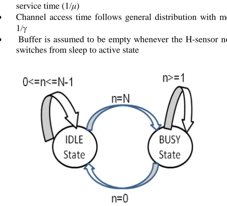
Fig. 2. Sub-operational states of H-sensor node during active state • Packets are delivered from H-sensor node to BS with mean
service time (1/μ)
• Channel access time follows general distribution with mean 1/γ
• Buffer is assumed to be empty whenever the H-sensor node switches from sleep to active state
Fig. 3. Two-state transition diagram of an L-sensor in idle state and busy state
All the H-sensors in all clusters during its period of active time will be in IDLE state or BUSY state. Here, an H-sensor node in a cluster, during its period of active time, remains in IDLE state, switches to BUSY state when the node’s buffer is filled at least with threshold number of packets (N)i.e., queue threshold and the node switches back from BUSY state to IDLE state when there are no packets in the buffer. The
two-and BUSY state is shown in figure 3. During BUSY state, the H-sensors deliver the packets to the BS. Such switching actions between IDLE state to BUSY state and BUSY state to IDLE state are referred to as transitions.The average energy consumption of an H-sensor node or CH depends on the queue threshold since most of the energy is consumed during transmission i.e., during BUSY state.
5.
PERFORMANCE ANALYSIS
In this section, we analyze the behavior of a single H-sensor node. As mentioned in section II, the arrival of data packets to H-sensors follows a Poisson process with mean arrival rate per
node (λ) and an H-sensor in a cluster during its period of active time, remains in IDLE state and switches to BUSY state when the H-sensor node’s buffer is filled at least with threshold number of packets (N) and switches back from BUSY state to IDLE state when there are no packets in the node’s buffer. We analyze the performance of the system in terms of the following parameters.
(a) Mean Delay:
Mean delay experienced by the packets in an H-sensor node is defined as the average waiting time of the packets in the queue. Based on M/G/1 queuing model, the mean number of packets in the queue (L) is determined as,
2 2 2 2
[
]
(
1)
2
[
]
2(1
)
2(
)
E S
N N
N
E D
L
N
λ
σ λ
ρ
ρ
σ
− +
+
= +
+
−
+
Where,
λ
ρ
µ
=
and
λ
σ
γ
=
Average Energy Consumption of an H-Sensor Node : During active time, the H-sensor node remains in IDLE state when the number of packets is less than the queue threshold. When the threshold value is reached due to the arrival of packets, the H-sensor node waits for the free channel for a mean channel access time 1/γ [13]. Once the channel is available, the node switches from IDLE state to BUSY state and transmits a preamble packet (271 bytes). Preamble packet is used for synchronization of an H-sensor node with the BS for the packet transmission [14]. After synchronization with the BS, the H-sensor node transmits all packets to BS from its buffer and switches back from BUSY state to IDLE state when the buffer gets empty. Hence a cycle during the active time of an H-sensor node constitutes,
• Arrival of data packets
• Duration of time spent for channel access Transition from IDLE state to BUSY state • Synchronization with the BS
• Transmission of packets to BS
• Transition from BUSY state to IDLE state
ISSN 2348 – 7968
CT Energy consumption due to transitions and synchronization in joules
E(N) Average energy consumption of an H-sensor node as a function of N in joules
E[I] Average duration of time the H-sensor node is in IDLE state
E[C] Average duration of cycle Ncy Number of cycles per unit time.
The value of queue threshold has significant effect on the average number of cycles or number of cycles per unit time (Ncy). The Ncy includes arrival of data packets, time spent on channel access, transitions, synchronization and transmission of packets. Since the focus of this paper is to reduce the average energy consumption during transmission based on queue threshold, the parameters that consumes energy during BUSY state are alone considered i.e., CT energy consumed due to transitions and synchronization and CH energy consumed during transmission. The energy consumed during sleep state, the energy consumed during idle mode and receive mode, the energy consumed during data generation and channel access time in active state are not considered. The average energy consumption of an H-sensor node E(N) is obtained and it is given by :
[ ]
[ ]
IE I
P
E C
=
Where
E I
[ ]
can be expressed as,1
[ ]
N
E I
λ γ
=
+
Using
P
I= −
1
ρ
and above equation we get[ ]
(1
)
N
E C
σ
λ
ρ
+
=
−
The number of cycles per unit time
( )
N
cy is given by1
[ ]
cyN
E C
=
Using the value
E C
[ ]
inN
cy, we get(1
)
cy
N
N
λ
ρ
σ
−
=
+
Now the average energy consumption of an H-sensor node
( )
E N
can be expressed as,
( )
H T cyE N
=
C L C N
+
This leads to the average energy consumption of an H-sensor node E(N) is obtained and it is given by :
(
1)
(2
)
(1
)
( )
2(
)
2(1
)
H T
N N
E N
C
C
N
N
ρ
ρ
σ
λ
ρ
σ
ρ
σ
−
−
−
=
+
+
+
+
−
+
6. EXPERIMENTAL RESULT USING
QUEUING MODEL
6.1 Average energy consumption:
Following are the parameter consider for calculating the average energy consumption
Table -1: Input Parameter for Average Energy Consumption
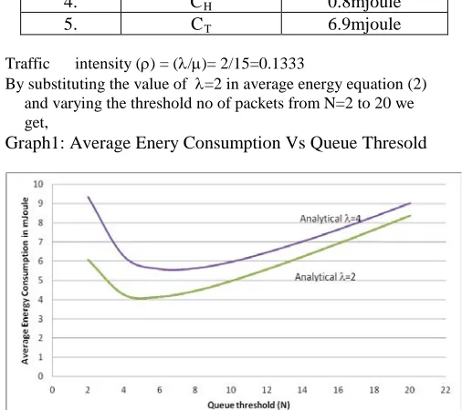
Traffic intensity (ρ) = (λ/µ)= 2/15=0.1333
By substituting the value of λ=2 in average energy equation (2) and varying the threshold no of packets from N=2 to 20 we get,
Graph1: Average Enery Consumption Vs Queue Thresold
Fig 6.1 Profile of Average Energy Consumption in m Joule and Queue Threshold (N) generated using M/G/1 model.
6.2
Mean Delay
For calculating the mean delay experienced by the packet in an H-sensor node is define as average waiting time of the packet in the queue. Following are the parameter consider for calculating the mean delay
Table -2: Input Parameter for Mean Delay
SR No. Notation/S ymbol
Meaning
1. λ 2 packet per CH per
Second
2. µ 15 msec per packet
3. N 2 to 20
4. CH 0.8mjoule
5. CT 6.9mjoule
SR No. Notation/Symbol Meaning
1. λ 2 packet per CH
per Second
2. µ 15 msec
3. N 2 to 20
4. CH 0.8mjoule
ISSN 2348 – 7968
Traffic intensity(ρ) = (λ/µ)= 2/15=0.1333
By substituting the value of λ=2 in mean delay equation (2)and varying the threshold no of packets from N=2 to 20 we get,
Graph2 : Mean Delay Vs Queue Threshold
Fig 6.2 Profile of Average Energy Consumption in m Joule and Queue Threshold (N) generated using M/G/1 model.
7. COMPARATIVE RESULT OF
ANALYTICAL AND SIMULATION
METHOD.
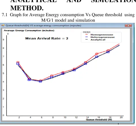
7.1 Graph for Average Energy consumption Vs Queue threshold using M/G/1 model and simulation
Fig. 7.1 Average energy Vs Queue threshold.
7.2 Graph for Queue Threshold Vs Mean Delay using M/G/1 model and simulation
Fig 7.2 Mean Delay Vs Queue Threshold(N)
The average energy consumption of a CH is determined for various values of N by assuming the mean arrival rate per CH as 2 and 4 by considering mean channel access time as 100 msec and it is shown in above Fig. From Fig.6.1 it is inferred that, as N increases, the average energy consumption per CH decreases and increases and minimum energy is consumed for the optimal threshold. The average energy consumption per CH decreases as N increases because, as N increases, the number of cycles per second decreases resulting in less energy consumption.
7.3 Comparative Result For Average Energy Consumption and Mean Delay When λ=2
Sr. No.
Value of Queue Threshold
Average Energy Consumption in
mjoule
Mean Delay in msec
By M/G/1 Queuing
Model
By Simulation
Model
By M/G/1 Queuing
Model
By Simulation
Model
1 N=2 6.0750 6.23 610 624 2 N=4 4.25 4.51 711 730 3 N=6 4.139 4.22 812 820 4 N=8 4.45 4.35 913 926 5 N=10 4.97 5.02 1014 1035 6 N=12 5.58 5.60 1115 1126 7 N=14 6.24 5.90 1137 1159 8 N=16 6.93 6.78 1237 1240 9 N=18 7.65 7.90 1337 1342 10 N=20 8.32 8.57 1519 1550
8. CONCLUSIONS
ISSN 2348 – 7968
network by taking channel contention into account using M/G/1 queuing model and the system performance in terms of average energy consumption and mean delay have been determined. We also compare the result of analytical method and simulation method by using queuing model. Hence it can be conclude that the analytical and simulation methods are produce same result. By using Queuing theory we can solve the real world problems.
REFERENCES
[1] Fuu-Cheng Jiang, Der-Chen Huang, Chao-Tung Yang, Fang-Yi Leu, “Lifetime Elongation for Wireless Sensor Network Using Queue-Based Approaches”, J Supercomput, Springer Science+Business Media, LLC, 2011. DOI 10.1007/s11227-010-0537-5.
[2] Tie Qiu, Lin Feng, Feng Xia, Guowei Wu, and Yu Zhou, “A Packet Buffer Evaluation Method Exploiting Queueing Theory for Wireless Sensor Networks”, ComSIS Vol. 8, No. 4, Special Issue, October2011, pp. 1027-1049. [3] Azmat Nafees, “Queuing theory and its application:
Analysis of the sales checkout Operation in ica supermarket” M.Sc. Thesis, Hogskolan Dalarna, University of Dalarna, June 2007.
[4] Zhi Quan, Ananth Subramanian and Ali H. Sayed, “REACA: An Efficient Protocol architecture for Large Scale Sensor Networks,” IEEE Transactions on Wireless Communications, vol. 6, no.10, October 2007, pp. 3846-3855. [5] J. Carle and D. Simplot-Ryl, “Energy-efficient area
monitoring for sensor networks,” IEEE Computer, vol. 37, no. 2, Feb. 2004, pp. 40–46.
[6] C. F. Chiasserini and M. Garetto, “An analytical model for wireless sensor networks with sleeping nodes,” IEEE Trans. Mobile Computing, vol. 5, no. 12, Dec. 2006, pp. 1706–1718.
[7] Vivek Mhatre, Catherine Rosenberg, “Homogeneous Vs. Heterogeneous Clustered Sensor Networks: A Comparative Study”, School of Electrical and Computer Eng., Purdue University, West Lafayette.
[8] E. Duarte-Melo and M. Liu, “Analysis of energy consumption and lifetime of heterogeneous wireless sensor networks,” in Proc. IEEE Globecom, Nov. 2002, pp.21-25. [9] V. Mhatre, C.P. Rosenberg, D. Kofman, “A minimum
cost heterogeneous sensor network with a lifetime constraint,” IEEE Trans. Mobile Computing, vol. 1, no.1, Jan. 2005, pp. 4-15.
[10] X. Du and Y. Xiao, “Energy efficient chessboard clustering and routing in heterogeneous sensor networks,” Int. Journal on Wireless Mobile Computing (IJWMC), vol.1, no. 2, Jan. 2006, pp. 121-130.
[11] X. Du and F. Lin, “Maintaining differentiated coverage in heterogeneous sensor networks,” EURASIP Journal on Wireless Comm. Networking, Oct. 2005, pp. 565-572. [12] M. Yarvis, N. kushalnagar, H. Singh,et al., “Exploiting