Protein Quantitation www.clinical.proteomics-journal.com
ExSTA: External Standard Addition Method for Accurate
High-Throughput Quantitation in Targeted Proteomics
Experiments
Yassene Mohammed, Jingxi Pan, Suping Zhang, Jun Han, and Christoph H. Borchers*
Purpose: Targeted proteomics using MRM with stable-isotope-labeled internal-standard (SIS) peptides is the current method of choice for protein quantitation in complex biological matrices. Better quantitation can be achieved with the internal standard-addition method, where successive increments of synthesized natural form (NAT) of the endogenous analyte are added to each sample, a response curve is generated, and the endogenous concentration is determined at thex-intercept. Internal NAT-addition, however, requires multiple analyses of each sample, resulting in increased sample consumption and analysis time.
Experimental design: To compare the following three methods, an MRM assay for 34 high-to-moderate abundance human plasma proteins is used: classical internal SIS-addition, internal NAT-addition, and external
NAT-addition—generated in buffer using NAT and SIS peptides. Using endogenous-free chicken plasma, the accuracy is also evaluated.
Results: The internal NAT-addition outperforms the other two in precision and accuracy. However, the curves derived by internal vs. external
NAT-addition differ by onlyࣈ3.8% in slope, providing comparable accuracies and precision with good CV values.
Conclusions and clinical relevance: While the internal NAT-addition method may be “ideal”, this new external NAT-addition can be used to determine the concentration of high-to-moderate abundance endogenous plasma proteins, providing a robust and cost-effective alternative for clinical analyses or other high-throughput applications.
Dr. Y. Mohammed, Dr. J. Pan, Dr. J. Han, Dr. C. H. Borchers University of Victoria - Genome British Columbia Proteomics Centre Victoria, Canada
E-mail: [email protected] Dr. Y. Mohammed
Center for Proteomics and Metabolomics Leiden University Medical Center Leiden, the Netherlands
The ORCID identification number(s) for the author(s) of this article can be found under https://doi.org/10.1002/prca.201600180 C
2017 The Authors.Proteomics–Clinical Application
Published by WILEY-VCH Verlag GmbH & Co. KGaA, Weinheim. This is an open access article under the terms of the Creative Commons Attribution-NonCommercial-NoDerivs License, which permits use and distribution in any medium, provided the original work is properly cited, the use is non-commercial and no modifications or adaptations are made.
DOI: 10.1002/prca.201600180
1. Introduction
During the past 25 years, proteomics has moved from a qualitative science to a quantitative one. Initially used for protein identification and modification site determination, it is now being advocated as an alternative to ELISA for clinical use.[1–5] Although relative
quantitation techniques are still in use and are still valuable for biomarker discovery, for biomarker verification, and clinical analysis, what is required are techniques that allow determination of the absolute amount of material present, so that the amount of protein in a patient sample analyzed in various clinical laboratories can be compared with normal levels. Although these quantitation techniques are sometimes called “absolute”, the concentrations in the biological sample are, in fact, determined by comparison to known amounts of standard materials.[6–9]
Ex-actly how this comparison is performed is the subject of this current paper.
MRM-based targeted proteomics is now widely accepted as a flexible, precise, and sensitive method for
Dr. S. Zhang MRM Proteomics Inc.
Victoria, British Columbia, Canada Dr. C. H. Borchers
University of Victoria
Department of Biochemistry and Microbiology Victoria, BC, Canada
Gerald Bronfman Department of Oncology Jewish General Hospital
Clinical Relevance
Many clinical cohort studies require rapid, deep, and multi-plexed analytical methods to match the extreme complexity of the collected samples and to allow high-throughput biomarker monitoring at low sample consumption. Targeted proteomics has been widely used to address these challenges when quanti-fying protein abundances in complex biological matrices. The “gold standard” quantitation method is the internal standard-addition method, where increasing amounts of synthesized natural form (NAT) of the proteotypic END peptides are added to each sample along with isotopically labeled internal stan-dard (SIS) at a fixed concentration for normalization, response curves are generated, and the END concentrations are deter-mined by extrapolation. This approach, however, requires mul-tiple analyses of each sample, resulting in increased sample consumption and analysis time. Our study of 34 plasma pro-teins showed that an “external” standard-addition—generated in buffer using NAT and SIS—can be used to determine the concentration of high-to-moderate abundance plasma pro-teins. While the internal standard-addition is the still best method, the standard curves derived with our external NAT-addition method differed by onlyࣈ3.8% in slope, resulting in comparable accuracy and precision values with good CVs, and provided a robust, precise, cost effective, and low sample-consuming alternative suitable for clinical applications.
absolute protein quantitation in complex biological samples,[10–16]
particularly when performed as part of a bottom-up approach using stable-isotope labeled analogues (SIS peptides) of the tar-get peptides as internal standards.[17,18]When SIS peptides are
used in conjunction with standard operating procedures (SOPs), reproducible results can be generated within and between lab-oratories, as the use of SIS peptides helps to compensate for instrumental drift and/or differences in matrix effects between samples,[19–21] as well as facilitating interference testing.[10,22,23]
Ideally, for the highest quantitative precision, the SIS peptide concentrations should be balanced to reflect the expected con-centrations in the particular matrix being studied (plasma, urine, cerebrospinal fluid (CSF), etc.).[24–27]The analyte intensities are
used in the downstream data analysis to determine the concen-trations of the surrogate peptides and thus the proteins of in-terest. Quantitation is typically done through linear regression analysis of the relative ratios of the internal standard (SIS) pep-tides to the endogenous (END) peppep-tides, i.e. SIS/END, using for a dilution series of the SIS peptide in a standard sample digest, prepared from a control or pooled sample.[23,25,28]The actual
con-centrations of the target analytes are determined by comparison with a calibration curve, where the relative responses of the END analyte and the spiked-in internal isotopically labeled standard (Figure 1A) are plotted as a function of concentration. These calibration curves also provide information on the linear dy-namic range of the assay and the uncertainties (CVs) in the measurements.
A less rigorous variant of this absolute quantitation method is where a single known concentration of SIS peptide is spiked into the sample, and the concentration in the sample is determined
from the ratio of the area of the END peak to the area of the la-beled peak. This approximation is possible because of the wide linear dynamic range of a triple quadrupole instrument—up to 5–6 orders of magnitude. This “single point” method makes the assumption that the calibration curve is linear within the region spanned by the SIS and the END peaks. Thus, the single-point method should be used with extreme caution and only over a dy-namic range of few orders of magnitude in concentration, where the instrument response is known to be linear from previous ex-periments.
In addition, while isotopically-labeled internal standards are considered to be chemically identical to the target analyte, and have identical retention times and fragmentation patterns, there have been occasions where SIS peptides do not entirely compen-sate for differences in matrix effects. These appear as “outliers” in previous studies,[23,29]and may be caused by a particular
sam-ple having a slightly different matrix composition (and potential interferences) than the reference sample used to generate the cal-ibration curve.
An alternative to quantification using calibration curves based on SIS peptides is to use the standard addition approach. In the standard addition method (a well-established technique in classi-cal analyticlassi-cal chemistry), a standard curve is generated by adding a series of different concentrations of the (unlabeled) target an-alyte to each sample. Thus, the standard curve is created in ex-actly the same matrix in which the analysis is performed. Specifi-cally, successive additions of the target analyte are made into each sample, followed by measuring the increasing responses result-ing from the increased amount of the analyte in the sample. A straight line fitting the data points is determined by linear re-gression, and the END concentration can be determined by the extrapolation of the regression line to thex-intercept. They-axis corresponds to the response, and thex-axis corresponds to the amount of analyte added (Figure 1B).
Although the term “standard addition” is sometimes used in-correctly in the literature, the key feature of the standard addition method (which differentiates it from other methods involving the addition of standards to a sample) is that varying concentrations of the target analyte—in its unlabeled form—are added to each sample. One of its obvious drawbacks of the internal standard ad-dition method (called the internal NAT-adad-dition method in this paper) is that it requires multiple analyses of each sample, which makes it impractical for LC/MS-based analyses of large numbers of research or clinical samples due to time and/or sample limita-tions. Thus, while standard addition is used in many branches of analytical chemistry (including colorimetry), and it is used fairly routinely in MS-based toxicology, it is not normally used in phar-macology or in clinical chemistry. It does, however, have clear advantages when matrices are complex or variable, or in the pres-ence of strong matrix effect.
The internal NAT-addition method has been used more of-ten for MALDI-based analyses—both of drugs and peptides— because of the speed and low sample requirements of this technique,[30–33]sometimes in combination with a labeled
inter-nal standard to compensate for instrument drift, as we did in our iMALDI study on angiotensin I.[34] Internal NAT addition
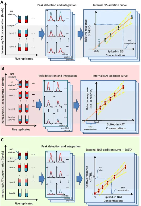
Figure 1. The three methods for generating standard curves. The method shown in panel A—the internal SIS-addition method—illustrates the common method for generating the standard curve in sample, which uses a SIS peptide mixture spiked in at several concentration levels. The calibration curve is generated by plotting the SIS/END peak area ratios as a function of SIS peptide concentration. The method shown in panel B shows the internal NAT-addition method where a concentration-balanced SIS peptide mixture (SISc) is spiked into the sample at a single concentration level and the NAT
is added at several concentration levels. The standard curve is generated by plotting the relative response (i.e., R(NAT+END)/RSISc), as a function of
the spiked-in NAT peptide concentration. The concentration of the END peptide is estimated by extrapolating the standard curve and determining the
x-intercept, of which the END concentration is the absolute value. Panel C shows the external NAT-addition method—ExSTA. In this method, the SISc
peptide mixture is spiked into buffer at a single concentration level, and varying levels of NAT are spiked into the mixture. The peak areas of the NAT and SIScpeptides are used (the END peptide is not present). After generating the calibration curve in buffer, the END peptide concentration in a sample is
estimated from a single point measurement of a sample, to which only a single concentration level of SIScpeptide has been added. The yellow lines in
effects in Stable Isotope Standards and Capture by AntiPeptide Antibodies (SISCAPA)-MALDI.[35]
Because the internal NAT-addition method requires multi-ple analyses of the same sammulti-ple, there have been relatively few applications of this method with LC/ESI–MS, even though this method has the advantage of compensating for matrix effects. Not surprisingly, most of these applications have been for cases where the biological matrix is particularly challenging (such as the analysis of tissues) or extremely variable (such as in postmortem or decomposed samples).[36,37]The internal
NAT-addition method has, however, been used occasionally to provide reference values for LC–MRM-based proteomic assays.[38]
Inter-nal NAT addition has also been used for LC/MS-based quanti-tation of small molecules in various tissues[39–42] and in
post-mortem blood.[37] A recent multiplexed MRM study used
stan-dard addition,[43] for the quantitative analysis of 115 veterinary
drugs in a variety of food matrices.
Here we compare the conventional method of adding a concentration-balanced SIS peptide mixture to each sample at multiple concentration levels (Figure 1A), with the internal stan-dard addition method (Figure 1B). Specifically, quantitation in the internal NAT-addition method is done by linear regression using a dilution series of the synthesized natural unlabeled form of the surrogate peptide (NAT) which is added to a sample where the END peptide is already present. The responses are normal-ized to the signal from the constant amount of SIS peptide which has been added to the sample.
In addition to these two methods, a third method is also evalu-ated. This new method, which we call the external NAT-addition method—external standard addition (ExSTA), is based on a stan-dard curve derived from unlabeled stanstan-dards spiked into buffer (Table 1and Figure 1C), again using a constant concentration of SIS peptide for normalization. Although using the same back-ground matrix as the sample is preferable, in real applications it is sometimes impractical, not affordable, or even impossible to obtain sufficient material to generate an internal SIS or NAT cal-ibration curve, as this would require a minimum of 18 injections (3 repeats of 6 levels). The question in such situations is whether an external NAT-addition method could be considered as an alternative.
2. Experimental Section
The three methods compared here are shown in Figure 1. For the internal SIS-addition method (Figure 1A), we spiked varying amounts of a mixture of 34 SIS peptides into a standard plasma sample to give a>100-fold range of concentrations (as in[44,45])
and measured the SIS/END response ratios for the END and heavy-labeled peptides.
For the internal NAT addition method (Figure 1B), we spiked 34 synthetic heavy-labeled SIS peptides representing the target proteins into a human plasma sample. The fixed concentra-tion of each SIS peptide was concentraconcentra-tion-balanced to be close to the END concentration of that peptide. We added the syn-thetic natural (unlabeled) forms (NAT) of these 34 peptides at 5 concentration levels, spanning a 100-fold concentration range, with level 3 being close to the END peptide concentrations. The (NAT+END)/SIS response ratios for the synthetic (NAT) plus
END peptide were calculated as:
Response(NAT+END)/ResponseSIS=R(NAT+END)/RSIS
For the external NAT-addition experiments (Figure 1C), we spiked a mixture of 34 SIS peptides into 0.1% FA in water at the same concentrations as would be expected in a plasma sample. We then spiked-in varying amounts of a concentration-balanced mixture of the 34 synthetic NAT peptides, to span a 100-fold con-centration range. The response ratios for the synthetic unlabeled peptide; i.e. NAT, and the corresponding SIS peptide were mea-sured as:
ResponseNAT/ResponseSIS=RNAT/RSIS
Standard curves were generated for all three methods and the concentrations were determined using Qualis-SIS, as described previously.[46]
For all calibration curves and standard curves, we used a weighted least-squares fitting approach to determine the slope andy-intercept of a straight line. The best-fit curves were ob-tained in an iterative four-step procedure (see Figure S1, Sup-porting Information). First, the best least-squares linear fit was calculated without weighting, followed by three similar fittings using weighting. The weights were generated for each step by using the standard curve from the previous iteration to calculate the reciprocal of the squared estimated value, i.e.(1/yi’)2 where
yi’ is the estimated value foryat concentration level i. Using this
strategy, we reached a stable standard curve after a total of four iterations, after which there were no further changes in the slope andy-intercept of the curve.
2.1. Internal SIS Addition (Varying Amounts of SIS and no NAT, in Plasma)
In the conventional internal SIS-addition method, we used our previously described approach[44,45]to determine the
concentra-tion of the END peptide. Briefly, we spiked in a series of increas-ing SIS concentrations across six levels coverincreas-ing a 1000-fold con-centration range. These data are used to generate a calibration curve based on a linear regression analysis of the peak area ratios in the sample. The ratio of SIS peak area to the END peak area is considered as the independent variable and the SIS concentra-tion at each level as the dependent variable. We used the curve to evaluate the dynamic range and to determine the concentration of the END peptide (Figure 1A).
2.2. Internal NAT Addition Method (Constant SIS and Varying Amounts of NAT, in Plasma)
Table 1.Characteristics of the three quantification methods described: internal SIS addition, internal NAT addition, and external NAT addition..
Internal SIS addition Internal NAT addition External NAT addition—ExSTA
Principle Standard curve based on SIS peptides added to each sample
Standard curve based on NAT and SIS peptides added to each sample
Standard curve based on NAT and SIS peptides added to buffer
Uses synthetic heavy labeled peptide (SIS)
Yes—for calibration curve Yes—for normalization only Yes—for normalization only
Uses synthetic light peptide (NAT) No Yes—for calibration curve Yes—for calibration curve
SIS dilution series is required Yes.
A series of SIS solutions are required with one concentration level in the middle of the curve (level D) being balanced to be as close as possible to the END concentration
No.
A single SIS solution is used, and its concentration is constant across all levels of the calibration curve. The concentration of each SIS peptide within the solution is balanced to be as close as possible to the END concentration in a representative sample.
No.
A single SIS solution is used, and its concentration is fixed across all levels. The concentration of each SIS peptide is balanced to be as close as possible to the expected END concentration in a representative sample.
Standard solutions NAT: not present
SIS: dilution series, 1:2:5:2:5:10 labeled F to A
NAT: dilution series, 1:2:5:2:5 labeled F to B
SIS: a single concentration-balanced solution
NAT: 1:2:5:2:5 labeled F to B SIS: a single concentration-balanced
solution
Generate curve in actual sample matrix
Yes
The standard curve is generated in the actual sample or a representative matrix.
Yes
The standard curve is generated in the actual sample (so matrix is identical to that of the sample)
No
The standard curve is generated in buffer
Suitable for small amount of sample No.
Multiple aliquots of the sample are required to generate a standard curve for each sample. (Typically 6 aliquots per sample, or 18 aliquots for replicate analyses)
No.
Multiple aliquots of the sample are required to generate a standard curve for each sample. (Typically 6 aliquots per sample, or 18 aliquots for replicate analyses)
Yes.
Number of analysis required per sample (for a 6 levels curve with 3 repeats/injections)
18 measurements per sample 18 measurements per sample Standard curve: 18 measurements in buffer
Analyses per sample: three replicates
Requires concentration-balancing of SIS to END in the reference sample
Recommended Not required Not required
of the SIS peptide. The END peptide concentration is then deter-mined by thex-intercept of the regression line (see Figure 1B).[47]
This approach uses a single fixed SIS concentration and series of increasing NAT concentrations across five levels covering a 100-fold concentration range. The SIS mixture is balanced to the ex-pected END concentrations in the sample.
2.3. External NAT-Addition Method–ExSTA (Constant SIS and Varying Amounts of NAT, in Buffer)
For this method (Figure 1C), we generated a standard addition curve in buffer using the same concentration-balanced SIS mix-ture and NAT amounts as in the internal NAT-addition method, i.e., a fixed SIS concentration and series of increasing NAT con-centrations across five levels covering a 100-fold concentration range. Using linear regression, we established the relationship between the peak area ratios, i.e., the RR at the different concen-trations as the dependent variable and the NAT concentration as the independent variable. We used the regression equation from this standard curve to calculate the concentration of the END
pep-tide in the sample by determining the RR of the peak area ratio when only the SIS peptide is spiked-in the sample (i.e., the RR for level A where there is no added NAT and where the peak signal in the light channel represents only the END peptide).
2.4. Chemicals and Reagents
For the internal standard experiments, we used human plasma obtained from BioreclamationIVT (catalogue number HM-PLEDTA2, lot number BRH796723). This plasma contained K2EDTA as an anticoagulant, and was obtained from healthy
race-and gender-matched consenting donors, aged 18–50. The tar-get panel used was composed of 34 peptides corresponding to high-to-moderate abundance plasma proteins, i.e. 20 fmol/μL to 200 pmol/μL (seeTable 2). All of these proteins are part of the PeptiQuant Workflow Performance Kit (MRM Proteomics, cat-alogue number WFPK-A6495-1) used to monitor LC/MRM–MS performance.[48]For each protein, one proteotypic surrogate
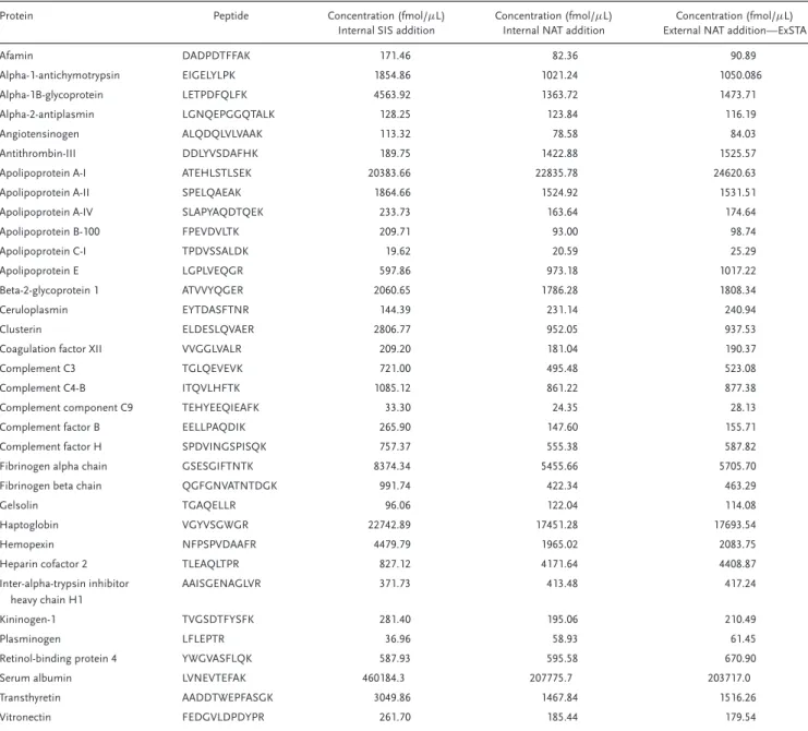
crite-Table 2.Proteotypic peptides used and their calculated concentrations with the three methods..
Protein Peptide Concentration (fmol/μL) Internal SIS addition
Concentration (fmol/μL) Internal NAT addition
Concentration (fmol/μL) External NAT addition—ExSTA
Afamin DADPDTFFAK 171.46 82.36 90.89
Alpha-1-antichymotrypsin EIGELYLPK 1854.86 1021.24 1050.086
Alpha-1B-glycoprotein LETPDFQLFK 4563.92 1363.72 1473.71
Alpha-2-antiplasmin LGNQEPGGQTALK 128.25 123.84 116.19
Angiotensinogen ALQDQLVLVAAK 113.32 78.58 84.03
Antithrombin-III DDLYVSDAFHK 189.75 1422.88 1525.57
Apolipoprotein A-I ATEHLSTLSEK 20383.66 22835.78 24620.63
Apolipoprotein A-II SPELQAEAK 1864.66 1524.92 1531.51
Apolipoprotein A-IV SLAPYAQDTQEK 233.73 163.64 174.64
Apolipoprotein B-100 FPEVDVLTK 209.71 93.00 98.74
Apolipoprotein C-I TPDVSSALDK 19.62 20.59 25.29
Apolipoprotein E LGPLVEQGR 597.86 973.18 1017.22
Beta-2-glycoprotein 1 ATVVYQGER 2060.65 1786.28 1808.34
Ceruloplasmin EYTDASFTNR 144.39 231.14 240.94
Clusterin ELDESLQVAER 2806.77 952.05 937.53
Coagulation factor XII VVGGLVALR 209.20 181.04 190.37
Complement C3 TGLQEVEVK 721.00 495.48 523.08
Complement C4-B ITQVLHFTK 1085.12 861.22 877.38
Complement component C9 TEHYEEQIEAFK 33.30 24.35 28.13
Complement factor B EELLPAQDIK 265.90 147.60 155.71
Complement factor H SPDVINGSPISQK 757.37 555.38 587.82
Fibrinogen alpha chain GSESGIFTNTK 8374.34 5455.66 5705.70
Fibrinogen beta chain QGFGNVATNTDGK 991.74 422.34 463.29
Gelsolin TGAQELLR 96.06 122.04 114.08
Haptoglobin VGYVSGWGR 22742.89 17451.28 17693.54
Hemopexin NFPSPVDAAFR 4479.79 1965.02 2083.75
Heparin cofactor 2 TLEAQLTPR 827.12 4171.64 4408.87
Inter-alpha-trypsin inhibitor heavy chain H1
AAISGENAGLVR 371.73 413.48 417.24
Kininogen-1 TVGSDTFYSFK 281.40 195.06 210.49
Plasminogen LFLEPTR 36.96 58.93 61.45
Retinol-binding protein 4 YWGVASFLQK 587.93 595.58 670.90
Serum albumin LVNEVTEFAK 460184.3 207775.7 203717.0
Transthyretin AADDTWEPFASGK 3049.86 1467.84 1516.26
Vitronectin FEDGVLDPDYPR 261.70 185.44 179.54
ria discussed previously,[49]and had been empirically optimized
and used in various previous studies and projects.[16,45,50]
The internal standard peptides are C-terminal isotopically la-beled tryptic peptides. These were synthesized in-house using a standard Fmoc procedure on an Overture peptide synthe-sizer (Protein Technologies; Woburn, MA, USA). Purification was performed by HPLC and confirmed by matrix-assisted laser desorption/ionization time of flight mass spectrometry (MALDI– TOF-MS) analysis, while characterization was performed by CZE and amino acid analysis (AAA). The AAA and CZE analyses en-abled us to determine the SIS peptide concentrations.
The corresponding natural forms of the 34 peptides were pur-chased from SynPeptide Co. Ltd. with purity higher than 90% for all peptides. Characterization of these 34 peptides was done by
CZE and AAA, which enabled us to accurately determine the NAT peptide concentrations. Other chemicals (e.g., ammonium bicar-bonate, and dithiothreitol) and solvents (e.g., acetonitrile and wa-ter) were LC–MS grade and were purchased from Sigma–Aldrich (St. Louis, MO, USA).
2.5. Sample Preparation
We followed a slightly modified version of the standard sample preparation of the PeptiQuant Workflow Performance Kit.[45]For
bonds were reduced with a 52.4 μL addition of 50 mM tris(2-carboxyethyl)phosphine for a final concentration of 5 mM. The sample was incubated in dry air at 60°C for 30 min, followed by alkylation of free sulfhydryl groups by adding 58μL of 100 mM iodoacetamide to give a final concentration of 10 mM, and incu-bating at 37°C for 30 min in the dark in a dry air incubator. To pre-vent alkylation of other residues, the remaining iodoacetamide was quenched by adding 58μL of 100 mM DTT and incubated at 37°C in a dry air incubator for 30 min. Proteolytic digestion was then initiated by adding an aliquot of TPCK (l-(tosylamido-2-phenyl) ethyl chloromethyl ketone)-treated bovine trypsin (Wor-thington; Lakewood, NJ, USA) at a 10:1 substrate/enzyme ra-tio. Digestion was allowed to proceed over night for 16 h at 37
°C. Upon digestion completion, acidified concentration-balanced SIS or SIS-NAT peptide mixture was added for the standard curve method (Figure 1A) and the standard addition method (Figure 1B) respectively. The six SIS mixtures were prepared in 0.1% FA solution to have six concentration levels of the SIS peptides spanning a 1000-fold concentration range, with a dilution series from the highest concentration of 1:2:5:2:5:10 (labeled F to A, from the highest to the lowest concentration), with level D be-ing balanced to be as close as possible to the END concentration. This dilution series was designed to cover a relatively wide con-centration range (1000), with the highest concon-centration designed to be 10 times as high as the average END peptide concentra-tion, and the lowest concentration to be 100 times lower than the average END peptide concentration. For the standard addition method, the SIS-NAT mixtures were prepared in 0.1% FA solu-tion to have six concentrasolu-tion levels of the NAT peptides, with a dilution series from the highest concentration of 1:2:5:2:5 for els F to B, and fixed concentrations of SIS peptides across all lev-els. The Level A sample was prepared in the same way but without adding any NAT and Level D contained equal amounts of SIS and NAT.
The six standard samples were prepared by combining aliquots of the plasma tryptic digest (200μL, containing 1.8μL of original undiluted plasma) with the SIS peptide mixture or the SIS-NAT mixture (98μL) and then the adding 202μL of 1% FA to each standard. After centrifugation at 12 000×gfor 10 min, 300μL of the supernatant was removed from the acid insoluble sodium deoxycholate, and then desalted and concentrated by SPE with an Oasis HLB cartridge using traditional vacuum manifold processing. The extractions were performed with vacuum bleed valve set to –25 kPa and a<1 mL/min flow rate. The eluted sam-ples (one per concentration level) were then frozen, lyophilized to dryness overnight, and rehydrated in 0.1% FA to give a final concentration of 1μg/μL (assuming an initial plasma protein concentration of 70 mg/mL) prior to injection. For the prepara-tion of the buffer samples, exactly the same SIS-NAT mixture was used, except that the standards are added to 0.1% FA instead of to the plasma digest.
2.6. LC/MRM–MS Analysis
LC/MRM-MS experiments were performed in quintuplicate, by reversed-phase UHPLC on a 1260 Infinity LC system using a Zorbax Eclipse Plus C18 Rapid Resolution HD column (150×
2.1 mm, 1.8μM particles; Agilent Technologies; Palo Alto, CA, USA). The column was maintained at 50°C and the autosam-pler was kept at 4°C. Mobile phase compositions of 0.1% FA in water for solution A and 100% ACN in 0.1% FA for B at a flow rate of 0.4 mL/min were used. The gradient was 0:2.7, 2:9.9, 15:17.1, 22:26.1, 25:40.5, 27:81, 29:81, and 30:2.7 (time, %B). The LC system was interfaced to a 6495 triple quadrupole mass spec-trometer (both from Agilent Technologies) via a standard-flow ESI source—see Table S1, Supporting Information for the list of the general acquisition parameters. Specific peptide parameters, such as collision energy and retention time, had been previously optimized and were not changed.[45]
2.7. Precision, Repeatability, and Correlation
The precision was evaluated as recommended by the FDA guidelines[51,52]at each concentration level by determining the CV
of quintuplicate measurements using the following equation:
CV=Standard deviation
Mean
The coefficients of determination (R2) for each standard curve
were used to evaluate the intra-batch repeatability and was deter-mined using the residual and total sum of squares as in following equation:
R2=1−Residual sum of squares
Total sum of squares =1−
i(yi− fi)2
i(yi−¯y)2
whereyiare the measured values, fiis the estimated values by
the standard curve, and ¯yis the mean of all measurements. To evaluate the closeness or discrepancy between the pro-tein concentrations determined using two different methods (method 1 and method 2), we determined both the Pearson and Spearman’s rank correlation coefficients using the following equations:
rperson=
i
x1i−x1
·x2i−x2
i
x1i−x1
2
·i
x2i−x2
2
where x1i and x2i the concentration values determined by
method 1 and method 2, andx1 andx2 are the mean concentra-tion values determined by method 1 and method 2 respectively. Spearman correlation coefficient was determined by the follow-ing equation:
rSpearman=
cov (rankx1,rankx2) σrankx1·σrankx2
=1−6
idi2
n3−n
Where cov is the covariance matrix, rankx1 is the rank vector
of the concentration values determined by method 1, similarly
r ankx2is the rank vector of the concentration values determined
by method 2,σrankx1andσrankx2are the standard deviations of the
rank vector of method 1 and 2. respectively,diis the difference
observations, i.e. the number determined protein concentrations by both methods.
2.8. Accuracy
In order to evaluate the accuracies of the three methods, the same experiment was repeated using chicken plasma instead of human plasma as the matrix. Chicken plasma was selected be-cause, with the exception of one peptide—YWGVASFLQK from retinol-binding protein 4 (a highly conserved protein between human and chicken)—all of the peptides used in our method were not present in the chicken proteome. We, nonetheless, kept the method unchanged and included retinol-binding pro-tein 4 in the LC–MRM/MS quantification, but it was excluded in the evaluation of the accuracy. The accuracies of the three types of calibration were determined based on the other 33 pep-tides, keeping the MRM method unchanged. For this test, we spiked a known amount of the natural form of each peptide into a chicken plasma sample. After digestion, the standards (SIS only for internal SIS-addition method, both SIS and NAT for inter-nal and exterinter-nal NAT-addition methods) were added to gener-ate the standard curves, as was done for the human samples. The accuracies of each method were calculated based on the known spiked-in amounts and the concentrations determined using each method’s calibration curve.
3. Results and Discussion
The three methods were compared on the basis of precision (as determined by the CVs of quintuplicate measurements), repeata-bility (as determined by the coefficients of determination), and the correlation between the determined concentrations.
3.1. Precision
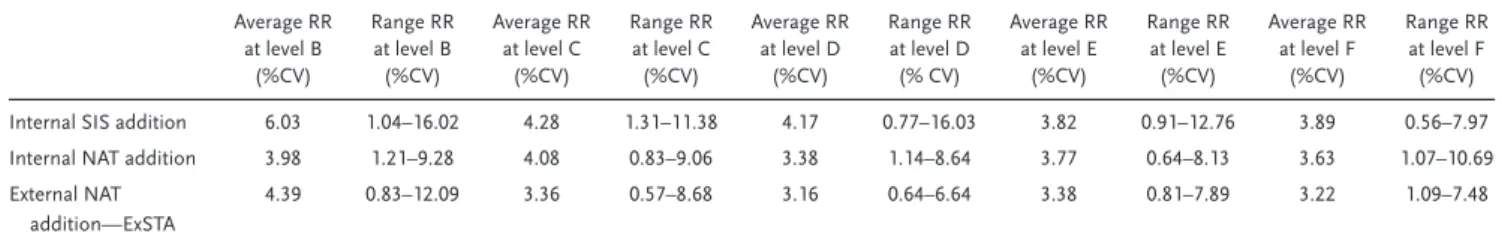
Table 3shows the average CVs of the relative response at each concentration level of all peptides. The average CV was 4.44% for the replicates in the internal SIS-addition method, 3.77% for the replicates in the internal NAT standard addition method, and 3.50% for the replicates in the external NAT-addition method. The values were calculated considering concentration levels F to B, which range from 10×the expected END concentration
to 0.01×the expected END concentration levels. One extreme outlier (DDLYVSDAFHK from antithrombin-III) in the external NAT-addition method was removed after it showed a difference of>5 SD at the lower concentration levels and 4 SD at levels F and E. The three methods, therefore, have similar precisions, but both the internal and external NAT-addition methods led to more precise measurements than the internal SIS-addition method. Comparing the maximum CVs across all concentration levels, the internal SIS-addition method had maximum CVs of 16.02 and 16.03% at concentration levels B and D, respectively, while the internal NAT addition method had a maximum CV of 10.69% for level F and maintained CVs of<10% for all other concentration levels. Similarly, the external NAT-addition method had its max-imum CV in level B (12.09%) and maintained<10% maximum CVs across all other concentration levels. The FDA guideline for the validation of bioanalytical chromatographic methods[51,52]sets
the acceptable precision limits at 15% of the nominal value. This shows that, even at their worst, the two standard addition meth-ods still met the FDA precision requirements for plasma proteins with high-to-moderate abundance.
3.2. Repeatability
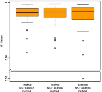
Three curves were generated for each peptide: one curve us-ing the internal SIS-addition method, one internal NAT addi-tion curve, and one external NAT-addiaddi-tion curve (Figure 1). For the internal SIS-addition method (Figure 1A), the coefficient of determination (R2) of the standard curve was between 0.9638
and 0.9987, with a mean of 0.9910 (Figure 2). The coefficients of determination for the external NAT-addition curves were be-tween 0.9623 and 0.9985, with a mean of 0.9912. For the internal NAT-addition curves, the coefficients of determination were be-tween 0.9671 and 0.9990, with a mean of 0.9902 (Figure 2). Only one peptide (DDLYVSDAFHK, from antithrombin-III) had anR2
value below 0.90 in buffer (i.e., with the external NAT-addition method).
The calculatedR2 values for the internal and external
NAT-addition methods included all of the measured points–i.e., we did not apply any level-removal strategy or impose any accu-racy and precision requirements (see 46 for details). This eval-uates the methods for accuracy and precision, and shows any possible deviation from acceptable ranges. In the internal SIS-addition method, generated by using only the balanced SIS pep-tide mixture, correspondingly highR2values were only observed
after applying precision and accuracy filters of 20% each, which
Table 3.A comparison of the CVs and the ranges of the measured relative responses (RRs) at each concentration level in the three methods used..
Average RR at level B
(%CV)
Range RR at level B (%CV)
Average RR at level C
(%CV)
Range RR at level C (%CV)
Average RR at level D
(%CV)
Range RR at level D (% CV)
Average RR at level E
(%CV)
Range RR at level E (%CV)
Average RR at level F
(%CV)
Range RR at level F (%CV)
Internal SIS addition 6.03 1.04–16.02 4.28 1.31–11.38 4.17 0.77–16.03 3.82 0.91–12.76 3.89 0.56–7.97
Internal NAT addition 3.98 1.21–9.28 4.08 0.83–9.06 3.38 1.14–8.64 3.77 0.64–8.13 3.63 1.07–10.69
External NAT addition—ExSTA
4.39 0.83–12.09 3.36 0.57–8.68 3.16 0.64–6.64 3.38 0.81–7.89 3.22 1.09–7.48
Figure 2. A box-and-whisker plot of theR2 values for the three
meth-ods used to generate the standard curves. One outlier in the external NAT-addition method—ExSTA, originated from antithrombin-III peptide DDLYVSDAFHK, had anR2value of 0.53. The spread of the boxplot
corre-sponds to the variability in the method.
removed any lower concentration levels that did not pass our ac-ceptance criteria (see 46 for details). Because all measurements were performed in quintuplicate at each concentration level, the mentionedR2values demonstrate the high intra-laboratory
tech-nical repeatability of all three methods.
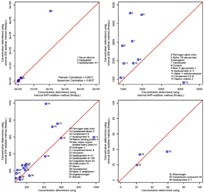
3.3. Concentration Correlation
The protein concentrations determined by the three methods are shown in Table 2.Figure 3shows the correlation between the internal SIS addition and the internal NAT-addition methods. The determined concentrations had a Pearson correlation coeffi-cient of 0.9972 and a Spearman correlation coefficoeffi-cient of 0.9037. The internal SIS-addition method and the internal NAT-addition method show an acceptable level of correlation. The concentra-tions values determined using the internal SIS-addition method were on average 1.44 times as high as those determined from the internal NAT-addition method, ranging from a minimum of 0.63 to a maximum of 2.35, with 26 out of the 34 peptides having concentrations higher in the internal SIS-addition method. This can also be seen in the slope of the regression equation: after re-moving five outliers—alpha-1B-glycoprotein, apolipoprotein A-I, clusterin, antithrombin-III, and heparin cofactor 2—the regres-sion equation between the two methods has a slope of 2.22 with ay-intercept of –284. While this is a good correlation, the high number of outliers is troublesome. Further investigations on the peptide levels of these five proteins will be necessary in order to find the source of the deviation between the two methods. For example, measuring these proteins with alternative peptides and comparing the results with those from the current peptides could help to identify interferences in any of the methods used. It is also important to keep in mind that an error could also originate
from incorrect AAA values—any error in the characterization of the SIS peptides would affect both methods similarly, but errors in the characterization of the NAT peptides would affect only the NAT addition method. However, we did not observe any indica-tion of a systematic error in the AAA values of the SIS and NAT peptides used.
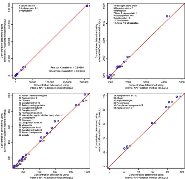
Figure 4shows the excellent correlation between the concen-trations determined from the internal and external NAT-addition methods with a Pearson correlation coefficient of 0.99994 and a Spearman correlation coefficient of 0.99939. It is evident that these two methods show very similar results, with only the two peptides at the lowest determined concentrations showing a rel-ative difference of>15%, and all differences being<23%. This shows that the external method can be used instead of the inter-nal NAT-addition method for quantitating peptides with concen-trations ofࣙ60 fmol/μL, with expected deviations of<15% from the concentrations that would have been obtained if the internal NAT addition approach had been used.
3.4. Matrix Effect and Slope Difference in Standard Curves
The slopes of the external NAT-addition curves in buffer were compared with those of the internal NAT-addition curves gener-ated in plasma (Figure S2, Supporting Information). There can be no direct comparison with the slope of the calibration curve in the internal SIS-addition method, because this method is based on addition of increasing SIS concentrations, while the internal and external standard additions involve addition of increasing NAT concentration, while keeping the SIS concentration for each pep-tide fixed.
The average difference in slope between the internal NAT-addition method and the external NAT-NAT-addition method was 3.8%, with a range of 0.14–12.45% (Report S1, Supporting In-formation). This means that the curves generated by both meth-ods using iterative linear regression are very similar. Thus, if the amount of a plasma sample is too small for an internal NAT-addition curve to be generated, a single-point measurement might be a method for determining the content of the sample. However, a single-point measurement approach can also be com-bined with an external standard curve in case of high-to-moderate abundance proteins to obtain information about the figures of merit for measuring a specific peptide from the external NAT-addition curve. This would add more confidence to the deter-mined concentration value of the protein. In addition, because the sensitivity of an MRM assay for a specific protein is character-ized by the slope of the standard curve,[53,54]the small difference
in slope between the internal and external NAT-addition meth-ods indicates that these two methmeth-ods have very similar nominal sensitivities.
3.5. Accuracy
Figure 3. Scatter plots showing the correlation between the concentrations determined by the internal SIS-addition method and the internal NAT-addition method. The four plots show four different plotting ranges and the corresponding measured peptide concentration in these ranges, these are 0 to 5e5 fmol/μL for the full range, 1000 to 5000 fmol/μL, 100 to 1000 fmol/μL, and 0 to 100 fmol/μL.
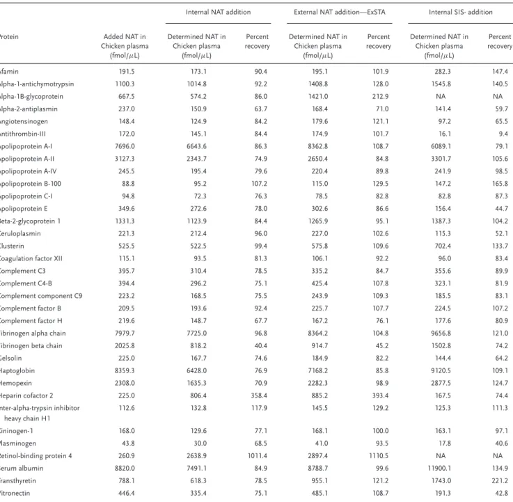
the concentrations, we generated one standard curve per pep-tide per method in chicken plasma (see Report 2, Supporting In-formation).Table 4 shows the amount of each unlabeled NAT peptide used for this experiment, along with the determined concentrations and the percent recoveries. The spiked-in pep-tide amounts varied from 44 fmol/μL to nearly 9000 fmol/μL, simulating the concentration ranges of authentic human plasma (i.e., 20 to ࣈ5000 fmol/μL) excluding three very high abun-dant proteins, i.e. serum albumin, apolipoprotein A-I, and hap-toglobin with concentration levels of above 17 (pmol/μL). With exception of two outliers, very good recoveries in all of the three methods were observed, with lower CVs in both of the internal and external NAT-addition methods compared to the
internal SIS-addition method. The two outliers were heparin co-factor 2 peptide (TLEAQLTPR), which we found to have strong in-terferences from chicken plasma, as well as retinol-binding pro-tein 4 peptide (YWGVASFLQK), which is also found in the con-served domain between the human and chicken retinol-binding protein 4.
Figure 4. Scatter plots showing the correlation between the concentrations determined by the internal and external NAT-addition methods, both using the same concentration-balanced SIS and NAT peptides. The four plots show four different plotting ranges and the corresponding measured peptide concentration in these ranges, these are 0 to 2e5 fmol/μL for the full range, 1000 to 5000 fmol/μL, 100 to 1000 fmol/μL, and 0 to 100 fmol/μL.
compared to the internal NAT-addition method. Table 4 and
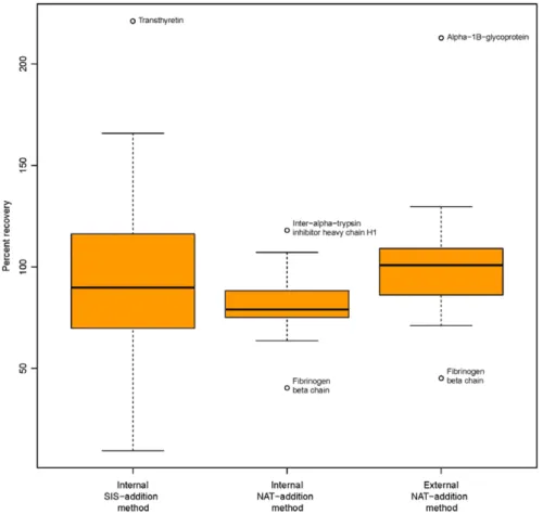
Figure 5 show that, while there is a fairly good mean per-cent accuracy obtained when using the SIS-addition method, the percent accuracy values have higher variability due to the wider spread of determined concentrations around the true pep-tide concentrations. Similarly, while the external NAT-addition shows a better mean accuracy value than the internal NAT-addition, the percent accuracy values have higher variability in the external NAT-addition method. In general, however, having tighter accuracy values with lower percent CVs is preferable, as it means that the error is less random and more system-atic, which can be corrected for when determining the actual concentration.
These accuracy values were obtained after removing the two outliers described above, and are based on all of the other values, including the extreme values appearing above and be-low the whiskers as shown in Figure 5. When removing these extreme values from all three methods (i.e., transthyretin, inter-alpha-trypsin inhibitor heavy chain H1, fibrinogen beta chain, and alpha-1B-glycoprotein), we observed mean per-cent recoveries of 81.9, 98.7, and 91.2% with CVs of 12.6, 14.6, and 40.1%, with the internal NAT addition, external NAT addition—ExSTA, and the internal SIS-addition methods, respectively.
Table 4.Determined accuracies for each of the three methods (internal NAT addition method, external NAT-addition method, and internal SIS-addition method) based on using known amount of unlabeled peptides (NAT) spiked into chicken plasma..
Internal NAT addition External NAT addition—ExSTA Internal SIS- addition
Protein Added NAT in
Chicken plasma (fmol/μL)
Determined NAT in Chicken plasma
(fmol/μL)
Percent recovery
Determined NAT in Chicken plasma
(fmol/μL)
Percent recovery
Determined NAT in Chicken plasma
(fmol/μL)
Percent recovery
Afamin 191.5 173.1 90.4 195.1 101.9 282.3 147.4
Alpha-1-antichymotrypsin 1100.3 1014.8 92.2 1408.8 128.0 1545.8 140.5
Alpha-1B-glycoprotein 667.5 574.2 86.0 1421.0 212.9 NA NA
Alpha-2-antiplasmin 237.0 150.9 63.7 168.4 71.0 141.4 59.7
Angiotensinogen 148.4 124.9 84.2 179.6 121.1 97.2 65.5
Antithrombin-III 172.0 145.1 84.4 174.9 101.7 16.1 9.4
Apolipoprotein A-I 7696.0 6643.6 86.3 8362.8 108.7 6089.1 79.1
Apolipoprotein A-II 3127.3 2343.7 74.9 2650.4 84.8 3301.7 105.6
Apolipoprotein A-IV 245.5 195.4 79.6 220.4 89.8 241.9 98.5
Apolipoprotein B-100 88.8 95.2 107.2 115.0 129.5 147.2 165.8
Apolipoprotein C-I 94.8 72.3 76.3 78.5 82.8 82.8 87.3
Apolipoprotein E 349.6 272.6 78.0 302.6 86.6 156.4 44.7
Beta-2-glycoprotein 1 1331.3 1123.9 84.4 1265.9 95.1 1387.3 104.2
Ceruloplasmin 221.3 212.4 96.0 227.0 102.6 115.3 52.1
Clusterin 525.5 522.5 99.4 575.8 109.6 702.4 133.7
Coagulation factor XII 115.1 93.5 81.3 106.1 92.2 96.0 83.4
Complement C3 395.7 310.4 78.5 335.2 84.7 355.6 89.9
Complement C4-B 394.4 296.2 75.1 425.4 107.8 323.1 81.9
Complement component C9 223.2 168.5 75.5 243.9 109.3 185.5 83.1
Complement factor B 209.5 193.6 92.4 225.7 107.7 224.5 107.2
Complement factor H 219.6 148.7 67.7 167.2 76.1 177.6 80.9
Fibrinogen alpha chain 7979.7 7725.0 96.8 8364.2 104.8 9656.8 121.0
Fibrinogen beta chain 2025.8 818.2 40.4 914.7 45.2 1502.8 74.2
Gelsolin 225.0 167.7 74.6 184.9 82.2 144.4 64.2
Haptoglobin 8359.3 6428.0 76.9 7168.2 85.8 9120.5 109.1
Hemopexin 2308.0 1635.3 70.9 2282.3 98.9 2877.5 124.7
Heparin cofactor 2 225.0 806.4 358.4 885.2 393.4 167.5 74.4
Inter-alpha-trypsin inhibitor heavy chain H1
112.6 132.8 117.9 145.5 129.2 125.3 111.3
Kininogen-1 168.0 129.6 77.1 168.1 100.0 163.1 97.1
Plasminogen 43.8 30.0 68.5 41.0 93.5 17.8 40.6
Retinol-binding protein 4 260.9 2638.9 1011.4 2897.4 1110.5 NA NA
Serum albumin 8820.0 7491.1 84.9 8788.7 99.6 11900.1 134.9
Transthyretin 788.1 618.3 78.5 955.1 121.2 1743.0 221.2
Vitronectin 446.4 335.4 75.1 485.1 108.7 191.3 42.8
within 15% of the nominal value (except at the LLOQ, where values with<20% accuracy are acceptable). Using the external standard addition method, we obtained a mean difference in concentration of 16.8% when using all peptides, except for the two peptides which showed interferences in chicken plasma. When removing the two extreme values in external standard addition method (i.e., alpha-1B-glycoprotein and fibrinogen beta chain, Figure 5), the mean difference dropped to 12.3% with a range between 0.04 and 29.6%. This indicates that accurate concentrations of END peptide surrogates for high-to-medium
abundance proteins in plasma samples can be obtained by per-forming single point measurements (i.e., where a single known amount of SIS mixture is spiked into the sample), in conjunction with external standard-addition curves generated in buffer, using a SIS-NAT mixture.
4. Conclusions
Figure 5. Boxplot of the percent recovery in each of the three methods, internal NAT addition, external NAT addition—ExSTA, and internal SIS-addition methods. Extreme values appearing as outliers are marked with the name of the corresponding protein.
standards is usually added to the tryptic sample digest and the responses from both the END and the heavy-labeled peptides are measured. This is the conventional internal SIS-addition method. Here we compared this conventional method with two standard-addition methods, in sample and in buffer. Both stan-dard addition methods showed less variability than the internal SIS-addition method. Although the quantitated targets in this current study are high-to-moderate abundance plasma proteins, we believe that this improvement is due to increases in the S/N ratios, should also improve the quantitation of low-abundance proteins.
Although the classical internal NAT-addition method is the best approach for generating a standard curve, it is impractical for routine analysis when the sample volume is limited. It also has a higher cost due to the use of SIS and NAT peptides for each sample at multiple concentration levels. Data acquisition times are also increased, because multiple analyses are required for each sample. The external NAT-addition technique—ExSTA described in this paper is a robust, fast, and cost-effective alter-native, resulting in an average difference from the slope of the internal NAT-addition curve of only 3.8%. It needs to be kept in mind that our results were not obtained on random peptides and transitions. In our opinion, the key to the success of the external NAT-addition method is that the peptides and transitions used have previously been carefully tested and were found to be inter-ference free in a pooled sample of target matrix.
An alternative to generating the external NAT-addition curve in buffer, external NAT-addition curves could also be generated in representative matrices, such as BSA in buffer, urine or CSF, or in pooled control samples, if available. In the absence of rep-resentative matrix, for instance in cases where pooled control is not available due to limited sample volume (as in tissue biopsies whereࣘ20μg of total protein is available for proteomics analy-sis), external standard addition technique in buffer offers a robust alternative.
Abbreviations
AAA,amino acid analysis;END,endogenous;ExSTA,external standard addition;NAT,synthesized natural form of the endogenous analyte;RR,
relative response;SIS,stable-isotope-labeled internal-standard
Supporting Information
Acknowledgments
Y. M. and J. P. contributed equally to this work. We are grateful to Genome Canada and Genome British Columbia for Science and Technology Inno-vation Centre support and for Genomics InnoInno-vation Network support to the University of Victoria - Genome British Columbia Proteomics Cen-tre through the Genome Innovations Network (204PRO for operations; 214PRO for technology development). MRM Proteomics Inc. thanks NRC-IRAP for project support. CHB is also grateful for support from the Leading Edge Endowment Fund. CHB is also grateful for support from the Segal McGill Family Chair in Molecular Oncology at the Jewish General Hospi-tal (Montreal, Quebec, Canada), and for support from both the Warren Y. Soper Foundation and the Alvin Segal Family Foundation to the Jewish General Hospital (Montreal, Quebec, Canada).
Conflict of Interest
Dr. Borchers is the Chief Scientific Officer of MRM Proteomics, Inc.
Keywords
ExSTA, external standard addition, Multiple Reaction Monitoring (MRM), quantitative proteomics, standard addition, standard curve
Received: April 25, 2017 Revised: August 9, 2017 Published online: October 25, 2017
[1] E. S. Boja, H. Rodriguez,Korean J. Lab. Med.2011,31, 61.
[2] C. E. Parker, T. W. Pearson, N. L. Anderson, C. H. Borchers,Analyst
2010,135, 1830.
[3] M. Palmblad, A. Tiss, R. Cramer,Proteomics Clin. Appl.2009,3, 6. [4] R. Apweiler, C. Aslanidis, T. Deufel, A. Gerstner, J. Hansen, D.
Hochstrasser, R. Kellner, M. Kubicek, F. Lottspeich, E. Maser, H. W. Mewes, H. E. Meyer, S. M¨ullner, W. Mutter, M. Neumaier, P. Nollau, H. G. Nothwang, F. Ponten, A. Radbruch, K. Reinert, G. Rothe, H. Stockinger, A. Tarnok, M. J. Taussig, A. Thiel, J. Thiery, M. Ueffing, G. Valet, J. Vandekerckhove, W. Verhuven, C. Wagener, O. Wagner, G. Schmitz,Clin. Chem. Lab. Med.2009,47, 724.
[5] A. J. Percy, A. G. Chambers, J. Yang, D. B. Hardie, C. H. Borchers,
Biochim. Biophys. Acta2014,1844, 917.
[6] M. A. Gillette, S. A. Carr,Nature Methods2013,10, 28.
[7] G. Di Conza, S. Trusso Cafarello, S. Loroch, D. Mennerich, S. De-schoemaeker, M. Di Matteo, M. Ehling, K. Gevaert, H. Prenen, R. P. Zahedi, A. Sickmann, T. Kietzmann, F. Moretti, M. Mazzone,Cell Rep. 2017,18, 1699.
[8] A. C. Uzozie, N. Selevsek, A. Wahlander, P. Nanni, J. Grossmann, A. Weber, F. Buffoli, G. Marra,Mol. Cell. Proteomics2017,16, 407. [9] J. Faktor, R. Sucha, V. Paralova, Y. Liu, P. Bouchal,Proteomics2017,
17, 1600323.
[10] P. Picotti, R. Aebersold,Nature Methods2012,9, 555.
[11] H. Keshishian, T. Addona, M. Burgess, D. R. Mani, X. Shi, E. Kuhn, M. S. Sabatine, R. E. Gerszten, S. A. Carr,Mol. Cell. Proteomics2009,
8, 2339.
[12] N. Selevsek, M. Matondo, M. S. Carbayo, R. Aebersold, B. Domon,
Proteomics2011,11, 1135.
[13] R. Schiess, B. Wollscheid, R. Aebersold,Mol. Oncol.2009,3, 33. [14] T. Fortin, A. Salvador, J. P. Charrier, C. Lenz, X. Lacoux, A. Morla, G.
Choquet-Kastylevsky, J. Lemoine,Mol. Cell. Proteomics2009,8, 1006. [15] D. Domanski, A. J. Percy, J. Yang, A. G. Chambers, J. S. Hill, G. V.
Cohen Freue, C. H. Borchers,Proteomics2012,12, 1222.
[16] A. J. Percy, A. G. Chambers, J. Yang, C. H. Borchers,Proteomics2013,
13, 2202.
[17] A. F. Altelaar, C. K. Frese, C. Preisinger, M. L. Hennrich, A. W. Schram, H. T. Timmers, A. J. Heck, S. Mohammed,J. Proteomics2013,88, 14. [18] E. Rodr´ıguez-Su´arez, A. D. Whetton,Mass Spectrom. Rev.2013,32, 1. [19] T. A. Addona, S. E. Abbatiello, B. Schilling, S. J. Skates, D. R. Mani, D. M. Bunk, C. H. Spiegelman, L. J. Zimmerman, A.-J. L. Ham, H. Keshishian, S. C. Hall, S. Allen, R. K. Blackman, C. H. Borchers, C. Buck, H. L. Cardasis, M. P. Cusack, N. G. Dodder, B. W. Gibson, J. M. Held, T. Hiltke, A. Jackson, E. B. Johansen, C. R. Kinsinger, J. Li, M. Mesri, T. A. Neubert, R. K. Niles, T. C. Pulsipher, D. Ransohoff, H. Ro-driguez, P. A. Rudnick, D. Smith, D. L. Tabb, T. J. Tegeler, A. M. Variy-ath, L. J. Vega-Montoto, A. Wahlander, S. Waldemarson, M. Wang, J. R. Whiteaker, L. Zhao, N. L. Anderson, S. J. Fisher, D. C. Liebler, A. G. Paulovich, F. E. Regnier, P. Tempst, S. A. Carr,Nat. Biotechnol.2009,
27, 633.
[20] S. E. Abbatiello, D. R. Mani, B. Schilling, B. Maclean, L. J. Zimmer-man, X. Feng, M. P. Cusack, N. Sedransk, S. C. Hall, T. Addona, S. Allen, N. G. Dodder, M. Ghosh, J. M. Held, H. V., H. D. Inerowicz, A. Jackson, H. Keshishian, J. W. Kim, J. S. Lyssand, C. P. Riley, P. Rud-nick, P. Sadowski, K. Shaddox, D. Smith, D. Tomazela, A. Wahlander, S. Waldemarson, C. A. Whitwell, J. You, S. Zhang, C. R. Kinsinger, M. Mesri, H. Rodriguez, C. H. Borchers, C. Buck, S. J. Fisher, B. W. Gib-son, D. Liebler, M. Maccoss, T. A. Neubert, A. Paulovich, F. Regnier, S. J. Skates, P. Tempst, M. Wang, S. A. Carr,Mol. Cell. Proteomics2013,
12, 2623.
[21] S. E. Abbatiello, B. Schilling, D. R. Mani, L. J. Zimmerman, S. C. Hall, B. MacLean, M. Albertolle, S. Allen, M. W. Burgess, M. P. Cusack, M. Ghosh, V. Hedrick, J. M. Held, H. D. Inerowicz, A. Jackson, H. Keshishian, C. R. Kinsinger, J. Lyssand, L. Makowski, M. Mesri, H. Rodriguez, P. Rudnick, P. Sadowski, N. Sedransk, K. Shaddox, S. J. Skates, E. Kuhn, D. Smith, J. R. Whiteaker, C. Whitwell, S. Zhang, C. H. Borchers, S. J. Fisher, B. W. Gibson, D. C. Liebler, M. J. MacCoss, T. A. Neubert, A. G. Paulovich, F. E. Regnier, P. Tempst, S. A. Carr,
Mol. Cell. Proteomics2015,14, 2357.
[22] S. A. Carr, S. E. Abbatiello, B. L. Ackermann, C. Borchers, B. Domon, E. W. Deutsch, R. P. Grant, A. N. Hoofnagle, R. H Uumlttenhain, J. M. Koomen, D. C. Liebler, T. Liu, B. Maclean, D. R. Mani, E. Mans-field, H. Neubert, A. G. Paulovich, L. Reiter, O. Vitek, R. Aebersold, L. Anderson, R. Bethem, J. Blonder, E. Boja, J. Botelho, M. Boyne, R. A. Bradshaw, A. L. Burlingame, D. Chan, H. Keshishian, E. Kuhn, C. Kinsinger, J. Lee, S. W. Lee, R. Moritz, J. Oses-Prieto, N. Rifai, J. Ritchie, H. Rodriguez, P. R. Srinivas, R. R. Townsend, J. Van Eyk, G. Whiteley, A. Wiita, S. Weintraub,Mol. Cell. Proteomics2014,13, 907. [23] H. Keshishian, T. Addona, M. Burgess, E. Kuhn, S. A. Carr,Mol. Cell.
Proteomics2007,6, 2212.
[24] M. A. Kuzyk, D. Smith, J. Yang, T. J. Cross, A. M. Jackson, D. B. Hardie, N. L. Anderson, C. H. Borchers,Mol. Cell. Proteomics2009,8, 1860.
[25] A. J. Percy, A. G. Chambers, C. E. Parker, C. H. Borchers,Met. Mol. Biol.2013,1000, 167.
[26] A. J. Percy, J. Yang, A. G. Chambers, R. Simon, D. B. Hardie, C. H. Borchers,J. Proteome Res.2014,13, 3733.
[27] A. J. Percy, J. Yang, D. B. Hardie, A. G. Chambers, J. Tamura-Wells, C. H. Borchers,Methods2015,81, 24.
[28] A. J. Percy, Y. Mohammed, J. Yang, C. H. Borchers,Bioanalysis2015,
7, 2991.
[29] A. J. Percy, A. G. Chambers, J. Yang, D. Domanski, C. H. Borchers,
Anal. Bioanal. Chem.2012,404, 1089.
[30] R. Szyszka, S. D. Hanton, D. Henning, K. G. Owens,J. Am. Soc. Mass Spectrom.2011,22, 633.
[31] S. Toghi Eshghi, X. Li, H. Zhang,Anal. Chem.2012,84, 7626. [32] S. Notari, C. Mancone, T. Alonzi, M. Tripodi, P. Narciso, P. Ascenzi,J.
Chromatogr. B2008,863, 249.
[34] D. R. Mason, J. D. Reid, A. G. Camenzind, D. T. Holmes, C. H. Borchers,Methods2012,56, 213.
[35] N. L. Anderson, M. Razavi, T. W. Pearson, G. Kruppa, R. Paape, D. Suckau,J. Proteome Res.2012,11, 1868.
[36] F. T. Peters, D. Remane,Anal. Bioanal. Chem.2012,403, 2155. [37] M. Gergov, T. Nenonen, I. Ojanper¨a, R. A. Ketola,J. Anal. Toxicol.2015,
39, 359.
[38] J.-S. Kim, T. L. Fillmore, T. Liu, E. Robinson, M. Hossain, B. L. Cham-pion, R. J. Moore, D. G. Camp, R. D. Smith, W.-J. Qian,Mol. Cell. Proteomics2011,10, M110.007302.
[39] U. Kuepper, F. Musshoff, B. Madea,Forensic Sci. Int.2011,207, 84. [40] E. J. Ahn, H. Kim, B. C. Chung, M. H. Moon,J. Sep. Sci.2007,30,
2598.
[41] I. Jim´enez-D´ıaz, F. Vela-Soria, A. Zafra-G´omez, A. Naval´on, O. Balles-teros, N. Navea, M. F. Fern´andez, N. Olea, J. L. V´ılchez,Talanta2011,
84, 702.
[42] F. Vela-Soria, I. Jim´enez-D´ıaz, R. Rodr´ıguez-G´omez, A. Zafra-G´omez, O. Ballesteros, A. Naval´on, J. L. V´ılchez, M. F. Fern´andez, N. Olea,
Talanta2011,85, 1848.
[43] M. E. Dasenaki, N. S. Thomaidis,Anal. Chim. Acta2015,880, 103. [44] A. J. Percy, A. G. Chambers, J. Yang, A. M. Jackson, D. Domanski, J.
Burkhart, A. Sickmann, C. H. Borchers,J. Proteomics2013,95, 66. [45] A. J. Percy, A. G. Chambers, D. S. Smith, C. H. Borchers,J. Proteome
Res.2013,12, 222.
[46] Y. Mohammed, A. J. Percy, A. G. Chambers, C. H. Borchers,J. Pro-teome Res.2015,14, 1137.
[47] W. R. Kelly, K. Pratt, W. F. Guthrie, K. R. Martin,Anal. Bioanal. Chem.
2011,400, 1805.
[48] A. J. Percy, J. Tamura-Wells, J. P. Albar, K. Aloria, A. Amirkhani, G. D. T. Araujo, J. M. Arizmendi, F. J. Blanco, F. Canals, J.-Y. Cho, N. Colom´ e-Calls, F. J. Corrales, G. Domont, G. Espadas, P. Fernandez-Puente, C. Gil, P. A. Haynes, M. L. Hern´aez, J. Y. Kim, A. Kopylov, M. Marcilla, M. J. McKay, M. Mirzaei, M. P. Molloy, L. B. Ohlund, Y.-K. Paik, A. Paradela, M. Raftery, E. Sabid´o, L. Sleno, D. Wilffert, J. C. Wolters, J. S. Yoo, V. Zgoda, C. E. Parker, C. H. Borchers,EuPA Open Proteomics
2015,8, 6.
[49] Y. Mohammed, D. Doma´nski, A. M. Jackson, D. S. Smith, A. M. Deelder, M. Palmblad, C. H. Borchers,J. Proteomics2014,106, 151. [50] M. A. Kuzyk, C. E. Parker, D. Domanski, C. H. Borchers,Methods Mol.
Biol.2013,1023, 53.
[51] U.S. Food and_Drug_Administration, US Department of Health and Human Services, Food and Drug Administration. Guidance for Industry Bioanalytical Method Validation. http://www.fda.gov/ downloads/Drugs/GuidanceComplianceRegulatoryInformation/ Guidances/ucm070107.pdf2001.
[52] U.S. Food and Drug Administration, Guidance for Industry Bioanalytical Method Validation - September 2013 Biopharmaceu-ticals http://www.fda.gov/downloads/drugs/guidancecompliance-regulatoryinformation/guidances/ucm368107.pdf 2013, July 26, 2015.