Algebra
A Computational Introduction
John Scherk
Copyright c
⃝
2009 by John Scherk
Some Rights Reserved
This work is licensed under the terms of the Creative Commons Attribution
--Noncommercial -- Share Alike 2.5 Canadalicense. The license is available athttp: //creativecommons.org/licenses/by-nc-sa/2.5/ca/
Attribution -- Noncommercial -- Share Alike
You are free:
To Share-- to copy, distribute and transmit the work
To Remix-- to adapt the work
Under the following conditions:
Attribution-- You must attribute the work in the manner spec-ified by the author or licensor (but not in any way that suggests that they endorse you or your use of the work).
Noncommercial-- You may not use this work for commercial purposes.
Share Alike-- If you alter, transform, or build upon this work, you may , distribute the resulting work only under the same or similar licence to this one.
With the understanding that:
Waiver-- Any of the above conditions can be waived if you get permission from
the copyright holder.
Other Rights-- In no way are any of the following rights affected by the license:
• Rights other persons may have either in the work itself or in how the work is used, such as publicity or privacy rights.
Notice-- For any reuse or distribution, you must make clear to others the license
Contents
Contents v
Preface xi
I Introduction to Groups
1
1 Congruences 3
1.1 Basic Properties . . . 3
1.2 Divisibility Tests . . . 5
1.3 Common Divisors . . . 9
1.4 Solving Congruences . . . 13
1.5 The Integers Modulon . . . 15
1.6 Introduction to Software . . . 18
1.7 Exercises . . . 21
2 Permutations 25 2.1 Permutations as Mappings . . . 25
2.2 Cycles . . . 27
2.3 Sign of a Permutation. . . 30
2.4 Exercises . . . 32
3 Permutation Groups 35
3.1 Definition . . . 35
3.2 Cyclic Groups . . . 37
3.3 Generators . . . 39
3.4 Software and Calculations . . . 42
3.5 Exercises . . . 47
4 Linear Groups 51 4.1 Definitions and Examples . . . 51
4.2 Generators . . . 54
4.3 Software and Calculations . . . 58
4.4 Exercises . . . 62
5 Groups 65 5.1 Basic Properties and More Examples . . . 65
5.2 Homomorphisms . . . 72
5.3 Exercises . . . 77
6 Subgroups 81 6.1 Definition . . . 81
6.2 Orthogonal Groups . . . 82
6.3 Cyclic Subgroups and Generators . . . 84
6.4 Kernel and Image of a Homomorphism . . . 90
6.5 Exercises . . . 92
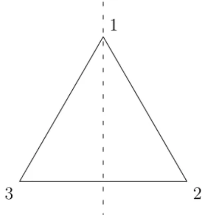
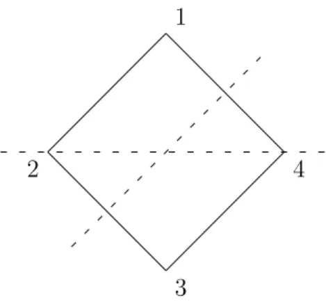
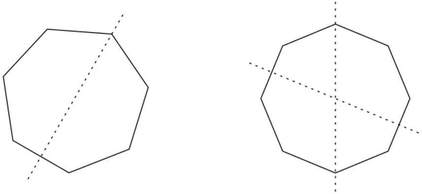
7 Symmetry Groups 97 7.1 Symmetries of Regular Polygons . . . 98
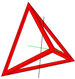
7.2 Symmetries of Platonic Solids . . . 101
7.3 Improper Symmetries. . . 106
7.4 Symmetries of Equations . . . 107
7.5 Exercises . . . 110
CONTENTS vii
8.1 Examples . . . 113
8.2 Orbits and Stabilizers . . . 115
8.3 Fractional Linear Transformations . . . 119
8.4 Cayley's Theorem . . . 123
8.5 Software and Calculations . . . 124
8.6 Exercises . . . 129
9 Counting Formulas 133 9.1 The Class Equation . . . 133
9.2 A First Application . . . 139
9.3 Burnside's Counting Lemma . . . 140
9.4 Finite Subgroups ofSO(3) . . . 142
9.5 Exercises . . . 148
10 Cosets 151 10.1 Lagrange's Theorem . . . 151
10.2 Normal Subgroups . . . 156
10.3 Quotient Groups . . . 159
10.4 The Canonical Isomorphism . . . 160
10.5 Software and Calculations . . . 164
10.6 Exercises . . . 171
11 Sylow Subgroups 175 11.1 The Sylow Theorems . . . 175
11.2 Groups of Small Order . . . 180
11.3 A List . . . 185
11.4 A Calculation . . . 186
11.5 Exercises . . . 188
12 Simple Groups 191 12.1 Composition Series . . . 191
12.3 Simplicity ofP SL(2,Fp). . . 196
12.4 Exercises . . . 200
13 Abelian Groups 203 13.1 Free Abelian Groups . . . 203
13.2 Row and Column Reduction of Integer Matrices . . . 207
13.3 Classification Theorems . . . 211
13.4 Invariance of Elementary Divisors . . . 215
13.5 The Multiplicative Group of the Integers Modn . . . 218
13.6 Exercises . . . 222
II Solving Equations
225
14 Polynomial Rings 227 14.1 Basic Properties of Polynomials . . . 22714.2 Unique Factorization into Irreducibles . . . 234
14.3 Finding Irreducible Polynomials . . . 236
14.4 Commutative Rings . . . 241
14.5 Congruences . . . 245
14.6 Factoring Polynomials over a Finite Field . . . 252
14.7 Calculations . . . 257
14.8 Exercises . . . 261
15 Symmetric Polynomials 267 15.1 Polynomials in Several Variables . . . 267
15.2 Symmetric Polynomials and Functions . . . 268
15.3 Sums of Powers . . . 274
15.4 Discriminants . . . 275
15.5 Software. . . 276
15.6 Exercises . . . 277
CONTENTS ix
16.1 Introduction . . . 281
16.2 Extension Fields . . . 283
16.3 Degree of an Extension . . . 286
16.4 Splitting Fields . . . 290
16.5 Cubics . . . 294
16.6 Cyclotomic Polynomials . . . 296
16.7 Finite Fields . . . 300
16.8 Plots and Calculations . . . 302
16.9 Exercises . . . 306
17 Galois Groups 311 17.1 Introduction . . . 311
17.2 Definition . . . 315
17.3 How Large is the Galois Group? . . . 318
17.4 The Galois Correspondence . . . 323
17.5 Discriminants . . . 337
17.6 Exercises . . . 339
18 Quartics 343 18.1 Galois Groups of Quartics . . . 343
18.2 The Geometry of the Cubic Resolvent . . . 347
18.3 Software. . . 351
18.4 Exercises . . . 352
19 The General Equation of thenth Degree 355 19.1 Examples . . . 355
19.2 Symmetric Functions . . . 357
19.3 The Fundamental Theorem of Algebra . . . 359
19.4 Exercises . . . 361
20.2 Cyclic Extensions . . . 367
20.3 Solution by Radicals in Higher Degrees . . . 370
20.4 Calculations . . . 375
20.5 Exercises . . . 376
21 Ruler-and-Compass Constructions 379 21.1 Introduction . . . 379
21.2 Algebraic Interpretation . . . 380
21.3 Construction of Regular Polygons . . . 385
21.4 Periods . . . 387
21.5 Exercises . . . 391
A Mathematica Commands 393
Bibliography 397
Preface
First Edition
This text is an introduction to algebra for undergraduates who are interested in
careers which require a strong background in mathematics. It will benefit
stu-dents studying computer science and physical sciences, who plan to teach
math-ematics in schools, or to work in industry or finance. The book assumes that
the reader has a solid background in linear algebra. For the first 12 chapters
el-ementary operations, elel-ementary matrices, linear independence and rank are
im-portant. In the second half of the book abstract vector spaces are used. Students
will need to have experience proving results. Some acquaintance with Euclidean
geometry is also desirable. In fact I have found that a course in Euclidean
geom-etry fits together very well with the algebra in the first 12 chapters. But one can avoid the geometry in the book by simply omitting chapter 7 and the geometric
parts of chapters 9 and 18.
The material in the book is organized linearly. There are few excursions away
from the main path. The only significant parts which can be omitted are those
just mentioned, the section in chapter 12 onP SL(2,Fp), chapter 13 on abelian
groups and the section in chapter 14 on Berlekamp's algorithm.
The first chapter is meant as an introduction. It discusses congruences and
the integers modulon. Chapters 3 and 4 introduce permutation groups and linear
groups, preparing for the definition of abstract groups in chapter 5. Chapters 8
and 9 are devoted to group actions. Lagrange's theorem comes in chapter 10 as
an application. The Sylow theorems in chapter 11 are proved following Wielandt
via group actions as well. In chapter 13, row and column reduction of integer
matrices is used to prove the classification theorem for finitely generated abelian
groups. Chapter 14 collects all the results about polynomial rings in one variable
over a field that are needed for Galois theory. I have followed the standard Artin
- van der Waerden approach to Galois theory. But I have tried to show where
it comes from by introducing the Galois group of a polynomial as its symmetry
group, that is the group of permutations of its roots which preserves algebraic relations among them. Chapters 18, 19, 20 and 21 are applications of Galois
theory. In chapter 20 I have chosen to prove only that the general equation
of degree5 or greater cannot be solved by taking roots. The correspondence
between radical extensions and solvable Galois groups I have found is often too
sophisticated for undergraduates.
This book also tries to show students how software can be used intelligently in
algebra. I feel that this is particularly important for the intended audience. There
is a delicate philosophical point. Does a software calculation prove anything?
This is not a simple question, and there does not seem to be a consensus among
mathematicians about it. There are a few places in the text where a calculation does rely on software, for example, in calculating the Sylow2-subgroups ofS8.
TheMathematica notebooks corresponding to the software sections are available
at the book's web site, as are the equivalentMapleworksheets.
Some of the exercises are referred to later in the text. These have been marked
with a bullet•. There are exercises where the software is useful but not essential,
and some where it is essential. However, I have deliberately not tried to indicate
which ones these are. Learning to decide when software is useful and when not,
seems to me to be an important part of learning to use it.
I am grateful to many people for help with this book at various stages, in
particular to Edward Bierstone, Imtiaz Manji, David Milne, Kumar Murty, Joe Repka and Paul Selick. In discussions over the years, Ragnar Buchweitz has made
many suggestions about teaching undergraduate algebra, for which I am most
xiii
several topics in the book suggested by him. The software was originally written
with the help of George Beck, Keldon Drudge and Petra Menz. The present
version is due to David Milne. The software which produced the pictures of the
Platonic solids in chapter 7 was also written by George Beck.
John Scherk
Toronto
2000
Second Edition
The first edition was published with CRC Press. This edition is published
on-line under the Creative Commons Copyright. The intention is to make the book
freely accessible to as many students and other readers as possible. The changes
in this edition are small. Many mistakes have been corrected. Some exercises
have been added and there are minor additions and refinements to the text.
John Scherk Toronto
Part I
Introduction to Groups
Introduction
The first part of this book is an introduction to group theory. It begins with a
study of permutation groups in chapter 3. Historically this was one of the starting
points of group theory. In fact it was in the context of permutations of the roots
of a polynomial that they first appeared (see 7.4). A second starting point was
the study of linear groups, i.e. groups of matrices, introduced in chapter 4. These appeared as groups of transformations which preserve different geometries, such
as Euclidean spaces, the hyperbolic plane (see8.8) or projective spaces. They also
arose as symmetry groups of objects like regular polygons or platonic solids in
in Euclidean space, discussed in chapter 7, or of tessellations of the Euclidean
or hyperbolic plane. The algebra underlying these special types of groups can be
1
Congruences
This is an introductory chapter. The main topic is the arithmetic of congruences,
sometimes called 'clock arithmetic'. It leads to the construction of the integers
modulo n. These are among the simplest examples of groups, as we shall see
in chapter 5. If nis a prime number, then the integers modulon form a field.
In chapter 4, we will be looking at matrices with entries in these fields. As an
application of congruences we also discuss divisibility tests. In order to be able to
solve linear congruences we review greatest common divisors and the Euclidean algorithm.
1.1
Basic Properties
Definition 1.1. Fix a natural number n. The integers a and b are congruent
modulonor modn, written
a≡b (mod n),
ifa−bis divisible byn.
For example,
23≡1 (mod 11)
23≡2 (mod 7)
23≡ −2 (mod 25)
If you measure time with a 12-hour clock, then you are calculating the hour
mod-ulo12. For example,5hours after9o'clock is not14o'clock but2o'clock. We
keep track of the days by reckoning modulo7. If today is a Wednesday, then10
days from today will be a Saturday. January 19 was a Wednesday in the year 2000.
To determine what day of the week it was in 1998, we can calculate
2·365 = 730≡2 (mod 7).
Therefore January 19 was a Friday in 1998. Calculating modulonis very similar
to calculating in the integers. First we note that congruence modulo n is an
equivalence relation.
Theorem 1.2. (i) a ≡a (mod n);
(ii) ifa≡b (mod n)thenb ≡a (mod n);
(iii) ifa≡b (mod n)andb≡c (mod n), thena≡c (modn).
It is easy to see why this is true. Clearlya−a= 0is divisible byn. Ifa−b
is divisible byn then so isb−a=−(a−b). And lastly, ifa−b andb−care
divisible by n, then so isa−c= (a−b) + (b−c).
Any integera is congruent to a unique integerr ,0 ≤ r ≤ n−1. Simply
divideabyn:
a=qn+r, for someqandr , 0≤r < n.
Thena ≡ r (mod n). From this you see thata is also congruent to a unique
integer between1andn, or between−57andn−58. Addition and multiplication
make sense modulon:
Theorem 1.3. (i) ifa≡b (mod n), andc≡d (mod n)thena+c≡b+d
(mod n);
(ii) ifa≡b (mod n), andc≡d (mod n)thenac≡bd (mod n);
1.2. DIVISIBILITY TESTS 5
1.2
Divisibility Tests
With these simple properties we can establish some divisibility tests for natural
numbers. Let's begin by deducing the obvious tests for divisibility by 2 and 5
using congruences. Suppose a is a natural number given in decimal form by
a=ak· · ·a1a0, in other words
a=ak10k+· · ·+a110 +a0
with0≤aj <10for allj. Then since10j ≡0 (mod 2)for anyj,
a≡a0 (mod 2).
Soais even if and only if its last digita0is even. Similarly10j ≡0 (mod 5)so
that
a≡a0 (mod 5).
Thusais divisible by5if and only ifa0 is, which is the case precisely whena0is
0or5. Next let's look at divisibility by3and9.
Test 1.4. Divisibility by3or9
(i) A natural numberais divisible by3if and only if the sum of its digits is divisible
by3.
(ii) A natural numberais divisible by9if and only if the sum of its digits is divisible
by9.
Proof. We have fork >0,
xk−1 = (x−1)(xk−1+· · ·+x+ 1).
Takingx= 10, we see that10k−1is divisible by9and in particular by3. So
10k≡1 (mod 9) and 10k ≡1 (mod 3).
Therefore if
then
a≡ak+· · ·+a1+a0 (mod 9) and a≡ak+· · ·+a1+a0 (mod 3).
Soais divisible by9, respectively3, if and only if the sum of its digits is divisible
by9, respectively3.
There is a test for divisibility by11which is similar. It is discussed in exercise
5. The tests for divisibility by7and13are more subtle. Here is the test for 7.
The test for13is in exercise6.
Test 1.5. Divisibility by7
Letabe a natural number. Writea = 10b+a0, where0 ≤ a0 < 10. Then ais
divisible by7if and only ifb−2a0 is divisible by7.
Proof. We have
10b+a0 ≡0 (mod 7)
if and only if
10b+a0 ≡21a0 (mod 7)
since 21a0 ≡0 (mod 7). Equivalently,
10b−20a0 ≡0 (mod 7),
i.e. 7divides 10b−20a0 = 10(b−2a0). Since10is not divisible by 7, this
holds if and only if7dividesb−2a0. In other words,
b−2a0 ≡0 (mod7).
For example,
426537183≡39≡0 (mod 3), but 426537183≡39≡3 (mod 9).
So426537183is divisible by3but not by9. And
1.2. DIVISIBILITY TESTS 7
Here is a table summarizing all the tests mentioned for a natural numbera. In
decimal form,ais given by ak10k+· · ·+a110 +a0 = 10b+a0.
n test
2 a0 even
5 a0 = 0or5
3 ak+· · ·+a1+a0divisible by3
7 b−2a0divisible by7
9 ak+· · ·+a1+a0divisible by9
11 ak− · · ·+ (−1)k−1a1+ (−1)ka0divisible by11
13 b+ 4a0divisible by13
There is another divisibility question with a pretty answer. When does a
nat-ural numberndivide10k−1for somek >0? Not surprisingly this is related to
the decimal expansion of1/n. First remember that every rational numberm/n
has a repeating decimal expansion (see [1],§6.1). This expansion is finite if and
only the prime factors of the denominatornare2and5. Otherwise it is infinite.
Ifn divides 10k −1, then the expansion of 1/n is of a special form. Suppose that
na= 10k−1, a ∈N.
Write out the decimal expansion ofa:
a=a110k−1+· · ·+ak−110 +ak.
So
a110k−1 +· · ·+ak−110 +ak =
10k
n −
1
n .
Divide this equation by10k:
0.a1. . . ak−1ak =
1
n −
10−k
Divide again by10k:
0.0| {z }. . .0
k
a1. . . ak=
10−k
n −
10−2k
n .
Continuing in this way, one gets
0.0| {z }. . . .0
ik
a1. . . ak =
10−ik
n −
10−(i+1)k
n ,
for anyi. Now sum overi:
0.a1. . . aka1. . . aka1. . . =
∞ ∑
i=0
(
10−ik
n −
10−(i+1)k
n ) = ( 1 n −
10−k
n
)∑∞
i=0
10−ik .
The sums converge because the series on the right is a geometric series. The sum
in the middle telescopes, leaving1/n, and the left hand side is a repeating decimal
fraction. So
1
n = 0.a1. . . aka1. . . aka1. . . . (1.1)
Conversely, it is easy to show that if1/n has a decimal expansion of this form,
thenn divides 10k−1. The shortest such sequence of numbersa
1, . . . , ak is
called the period of 1/n and k the length of the period. If we have any other expansion for1/n,
1
n = 0.b1. . . blb1. . . blb1. . . ,
for someb1, . . . , bl, then we see that lmust be a multiple of the period. So the
answer to our original question is:
Theorem 1.6.
10k−1≡0 (mod n)
if and only if1/nhas a decimal expansion of the form(1.1)andkis a multiple of the length
1.3. COMMON DIVISORS 9
Takingn= 7, we can calculate that
1
7 = 0.142857142857. . . .
So1,4,2,8,5,7is the period of1/7, which has length6. Then106−1 = 999999
is divisible by7, and for no smallerkis10k−1divisible by7.
1.3
Common Divisors
Recall thatdis acommon divisor of two integersaandb(not both0) ifddividesa
andddividesb. Thegreatest common divisor is the largest one and is written(a, b).
Every common divisor ofaandbdivides the greatest common divisor. We can
compute(a, b)by theEuclidean algorithm. We dividea by bwith a remainderr. Then we dividebbyrwith a remainderr1, and so on until we get a remainder0.
a=qb+r 0≤r < b
b =q1r+r1 0≤r1 < r
..
. ...
ri−1 =qi+1ri+ri+1 0≤ri+1 < ri
..
. ...
rn−2 =qnrn−1+rn 0≤rn< rn−1
rn−1 =qn+1rn
In chapter 14 we shall see the same algorithm for polynomials. The reason that this algorithm computes(a, b)is the following:
Lemma 1.7. Letuandv be integers, not both0. Write
u=qv+r ,
for some integersqandrwith 0≤r <|v|. Then
Proof. Ifd is a common divisor of u and v, thend dividesr = u−qv and is
therefore a common divisor ofv andr. Conversely, ifdis a common divisor of
vandr, thenddividesu =qv+rand is therefore a common divisor ofuand
v. So the greatest common divisor of the two pairs must be the same.
Applying this to the list of divisions above we obtain
(ri−1, ri) = (ri, ri+1)
for eachi < n. Now the last equation says thatrn|rn−1. This means that
(rn−1, rn) =rn.
Therefore arguing by induction,
(ri−1, ri) =rn
for alli, in particular
(a, b) =rn.
The proof of the lemma also shows that any common divisor ofaandbdivides
(a, b).
We can read more out of the list of equations. The first equation tells us thatr
is a linear combination ofaandb. The second one, thatr1is a linear combination
ofbandr, and therefore ofaandb. The third, thatr2is a linear combination of
r1andr, and therefore ofaandb. Continuing like this, we get thatrnis a linear
combination ofaandb. Thus there exist integerssandtsuch that
(a, b) = sa+tb .
Example 1.8. Takea = 57andb = 21. Then
57 = 2·21 + 15
21 = 15 + 6
15 = 2·6 + 3
1.3. COMMON DIVISORS 11
Therefore
3 = (57,21).
Furthermore
15 = 57−2·21
6 = 21−15 =−57 + 3·21
3 = 15−2·6 = 3·57−8·21.
So we can takes= 3andt=−8. △
Another way to look at the Euclidean algorithm is as an algorithm which expresses the rational numbera/bas a continued fraction. We have
a
b =q+
r
b =q+
1 ( b r ). But b
r =q1+ r1
r ,
so
a
b =q+
1
q1+
r1
r
=q+ 1
q1+
1 ( r r1 ) .
Continuing like this, our list of equations gives us the continued fraction
a
b =q+
1
q1+
1
. ..
qn+
1
In our example, we find that
57
21 = 2 + 1
1 + 1
2 + 1 2
For more about the origins of the Euclidean algorithm, and its connection with
the rational approximation of real numbers, see [2]. To read more about
contin-ued fractions in number theory, see [1].
Returning to the greatest common divisor, we say thata and b arerelatively
primeif(a, b) = 1, that is, if they have no common divisors except±1. Thus, if
aandbare relatively prime, there exist integerssandtsuch that
1 = sa+tb .
For example,16and35are relatively prime and
1 =−5·35 + 11·16.
Related to the greatest common divisor of two integers is their least common
multiple. The least common multiple m of a, b ∈ Zis the smallest common
multiple ofaandb, i.e. the smallest natural number which is divisible by botha
andb. We shall write
m=lcm(a, b).
It is not hard to see thatmdivides every common multiple ofaandb, and that
ab
(a, b) =lcm(a, b).
In example1.8above,
1.4. SOLVING CONGRUENCES 13
1.4
Solving Congruences
It is very useful to be able to solve linear congruences, just the way you solve
linear equations.
Theorem 1.9. If(a, n) = 1, then the congruence
ax≡b (mod n)
has a solution which is unique modulon.
Proof. Write1 = as+ntfor some integerssandt. Thenb =bas+bnt. Thus
b ≡abs (mod n)
and x = bsis a solution of the congruence. If we have two solutionsx andy
thenax ≡ ay (mod n)i.e. n dividesax−ay = a(x−y). Sinceaand nare
relatively prime, this means thatndividesx−y. Thusx≡y (mod n).
Example 1.10. Let's solve the congruence
24x≡23 (mod 31).
First we use the Euclidean algorithm to find integerssandtsuch that24s+31t= 1. One such pair iss=−9andt= 7. Then
23 = 24(23s) + 31(23t)
so that
24(23s)≡23 (mod 31).
Thus x = −207 ≡ 10 (mod 31) is a solution of the congruence. We could
also just compute multiples of24modulo31. △
In particular the congruenceax≡1 (mod n)has a solution, unique modulo
n,
Remark1.11. If nis prime, then allawith a ̸≡ 0 (modn)are relatively prime
tonand have 'multiplicative inverses' modn.
Notice however that
9x≡1 (mod 36)
does not have a solution. For if such anxdid exist we could multiply the
con-gruence by4and get
0≡4·9x≡4 (mod 36).
But0−4is not divisible by36. In fact it is true in general, that ifa andn are
not relatively prime, then
ax≡1 (mod n)
does not have a solution. For suppose thata = a′dand n = n′dwith d > 1.
Thenn′a=n′a′d≡0 (mod n)so that
0≡n′ax≡n′ ̸≡0 (mod n).
Therefore no suchxcan exist.
In general we letφ(n)denote the number of integersa,0 < a ≤n, which
are relatively prime ton. For example ifpis prime thenφ(p) = p−1.
Later we will also need to solve simultaneous congruences. The result which
tells us that this is possible is called the Chinese Remainder Theorem.
Theorem 1.12. Ifn1 andn2 are relatively prime, then the two congruences
x≡b1 (mod n1) and x≡b2 (mod n2)
have a common solution which is unique modulon1n2.
Proof. A solution of the first congruence has the formb1+sn1. For this to be a
solution of the second congruence, we must have that
1.5. THE INTEGERS MODULON 15
Since(n1, n2) = 1, the previous theorem assures us that such ansexists. If x
andyare two solutions, thenx≡y (mod n1)andx≡y (mod n2), i.e. x−y
is divisible by n1 and byn2. Asn1 and n2 are relatively prime,x−y must be
divisible byn1n2. Thusx≡y (mod n1n2).
Example 1.13. Solve
x≡14 (mod 24)
x≡6 (mod 31)
.
Solutions of the first congruence are of the form14 + 24s. So we must solve
14 + 24s≡6 (mod 31)
or equivalently
24s≡23 (mod 31).
This is the congruence we solved in example 1.10. We saw that s = 10 is a
solution. Therefore x = 254 as a solution of the two congruences we began
with. △
1.5
The Integers Modulo
n
As pointed out in theorem1.2, congruence modulonis an equivalence relation.
The equivalence classes are called congruence classes. The congruence class of
an integerais
¯
a := a+nZ := {a+sn|s∈Z}
The set of all congruences classes is denoted by Z/nZand called the set ofintegers
modulon. Since every integerais congruent to a uniquersatisfying 0≤r < n,
¯
between Z/nZ and {0,1, . . . , n − 1}. For example, in Z/2Z there are two
congruence classes:
0 + 2Z = {2s|s ∈Z},
the even integers, and
1 + 2Z = {1 + 2s |s∈Z},
the odd integers. We can define addition onZ/nZby
¯
a+ ¯b = a+b .
Because of theorem1.2this makes sense. You can think of this as adding two
natural numbers a and b in {0,1, . . . , n− 1} modulo n, i.e., their sum is the
remainder after division ofa+bbyn. This addition inZ/nZis associative and
commutative:
(¯a+ ¯b) + ¯c = ¯a+ (¯b + ¯c)
¯
a+ ¯b = ¯b+ ¯a .
And
¯
a+ ¯0 = ¯0
¯
a+ (−a) = ¯0.
For example, inZ/10Z,
¯
5 + ¯7 = ¯2, ¯4 + ¯6 = ¯0.
Multiplication can also be defined onZ/nZ:
¯
a·¯b := ab .
As with addition we can think of this as just multiplication modulon for two
numbers from{0,1, . . . , n−1}. It too is associative and commutative, and ¯1
1.5. THE INTEGERS MODULON 17
multiplicative inverse. For example, we checked that inZ/36Zthe multiplicative
inverse of¯7is31. We also saw that because¯4·¯9 = ¯0, ¯9has no multiplicative
inverse.
We have seen thatZ/nZ, at least whennis prime, has many formal properties
in common with the set of real numbersR and complex numbers C. We can
collect these properties in a formal definition.
Definition 1.14. A fieldF is a set with two binary operations, called 'addition'
and 'multiplication', written+and·respectively, with the following properties (a
binary operation onF is just a mapping F ×F →F):
(i) Addition and multiplication are both associative and commutative;
(ii) Fora, b, c∈F,a(b+c) =ab+ac;
(iii) There exist distinct elements 0,1∈F such that for anya∈F,
a+ 0 =a
a·1 = a .
(iv) For anya∈F there exists a unique element, written−a, such that
a+ (−a) = 0,
and for anya∈F, a̸= 0, there exists a unique element, writtena−1, such
that
a·a−1 = 1.
These are the formal properties satisfied by addition and multiplication inR andC, as well as inZ/pZforpprime. We introduce the notationFp forZ/pZ.
As pointed out above, ifnis not prime, then not all non-zero elements inZ/nZ
1.6
Introduction to Software
The main purpose of this section is to give you a chance to practice using
Math-ematica. It has several functions which are relevant to this section. For making
computations in the integers modulonthere is a built-in functionMod. Thus
In[1]:= Mod[25+87,13]
Out[1]= 8
and
In[2]:= Mod[2^12,7]
Out[2]= 1
A more efficient way of computing powers modnis to use the functionPowerMod:
In[3]:= PowerMod[2,12,7]
Out[3]= 1
For any real numberathe functionN[a, m]will compute the firstmdigits ofa. For example,
In[4]:= N[1/7, 20]
Out[4]= 0.14285714285714285714
So we see that the period of 1/7is 1,4,2,8,5,7, as discussed above. Similarly
1.6. INTRODUCTION TO SOFTWARE 19
Out[5]= 0.0526315789473684210526315789473684210526
Thus the period of1/19 is 0,5,2,6,3,1,5,7,8,9,4,7,3,6,8,4,2,1 , which
has length18. And
In[6]:= Mod[10^18 - 1, 19]
Out[6]= 0
but for smallerk,10k−1̸≡ 0 (mod 19). We can do these calculations for all
the primes less than30say, and tabulate the results. They confirm theorem1.6.
prime 3 7 11 13 17 19 23 29
length of period 2 6 2 6 16 18 22 28 smallest k 2 6 2 6 16 18 22 28
Interestingly
1001 = 103+ 1 = 7·11·13,
so that
103+ 1 ≡0 (mod 7).
Similarly,
In[7]:= Mod[10^9+1, 19]
Out[7]= 0
What do you think is going on? Experiment a bit and try to make a conjecture.
Given a pair of integers aand b, the function ExtendedGCDwill compute
In[8]:= ExtendedGCD[57, 21]
Out[8]= {3,{3,-8}}
This means that3 = 3·57−8·21. If we want to find the multiplicative inverse of105inF197, we can enter
In[9]:= ExtendedGCD[105, 197]
Out[9]= {1,{-15,8}}
So 1 =−15·105 + 8·197and−15 = 182is the multiplicative inverse of105.
There is a function called ChineseRemainder which will solve two such congruences simultaneously. In fact it will solve a system:
x≡b1 (mod n1)
.. .
x≡br (mod nr)
Simply enter
In[10]:= ChineseRemainder[{b1, ... , br},{n1, ...
, nr}]
So in our example:
In[11]:= ChineseRemainder[{14, 6},{24, 31}]
1.7. EXERCISES 21
1.7
Exercises
1. On what day of the week will January 19 fall in the year 2003?
2. Solve the following congruences:
a) 5x≡6 (mod 7)
b) 5x≡6 (mod 8)
c) 3x≡2 (mod 24)
d) 14x≡5 (mod 45).
3. Solve the following systems of congruences:
a) 5x≡6 (mod 7)and5x≡6 (mod 8)
b) 14x≡5 (mod 45)and4x≡5 (mod23).
Check whether theMathematicafunctionChineseRemaindergives the same answers as you get by hand.
4. •Forpprime,0< k < p, show that
a) (
p k
)
≡0 (mod p) ;
b)
(x+y)p ≡xp +yp (mod p).
5. Prove that a natural numbera is divisible by11if and only if the alternating
sum of its digits is divisible by11.
6. Show that10m+n,0 ≤n < 10, is divisible by13if and only ifm+ 4nis
7. Prove that a rational numberm/n, wheremandnare integers,n ̸= 0, has a
finite decimal expansion if and only if the prime factors ofnare2and5.
8. Letnbe a natural number. Suppose that1/nhas a decimal expansion of the
form0.a1. . . aka1. . . aka1. . .. Prove thatn|(10k−1).
9. For each primep < 30, find the smallestk ∈Nsuch that
10k+ 1≡0 (mod p),
and compare it with the length of the period of1/p.
10. Letpbe a prime number, and letkbe the length of the period of1/p. Suppose
thatk = 2l is even. Prove that 10l + 1is divisible byp, and that 10m + 1
is not divisible bypfor anym < l. (Suggestion: write 102l−1 = (10l− 1)(10l+ 1).)Does this hold true ifpis a composite number?
11. •Make a table ofφ(n)forn ≤20. Forpprime,r≥1, calculateφ(pr).
12. Suppose that you have a bucket that holds 57cups, and one that holds 21
cups. How could you use them to measure out3cups of water?
13. Given integersaandbwhich are relatively prime, suppose that
sa−tb= 1,
for some integerssandt. Suppose that
s′a−t′b= 1,
as well, for some integerss′ andt′. Prove that there then exists an integerk
such that
s′ =s+kb and t′ =t+ka .
1.7. EXERCISES 23
a) Show that lcm(a, b)divides every common multiple ofaandb.
b) Suppose that(a, b) = 1. Prove that then lcm(a, b) = ab.
c) Prove that in general
lcm(a, b) = ab (a, b) .
15. Write out addition and multiplication tables forZ/6Z. Which elements have
multiplicative inverses?
16. Write out the multiplication table forZ/7Z. Make a list of the multiplicative
inverses of the non-zero elements.
17. How many elements ofZ/7ZandZ/11Zare squares? How many elements
ofZ/pZ, wherepis prime, are squares? Make a conjecture and then try to
prove it.
18. Suppose thatn∈Nis a composite number.
a) Show that there exista, b∈Zwith¯a,¯b̸= 0 ∈Z/nZ, but¯a¯b= 0.
b) Prove thatZ/nZis not a field.
19. •Let
Q(√2) = {a+b√2|a, b∈Q} ⊂R.
Verify thatQ(√2)is a field.
20. Let
C=
{(
a b
−b a
)
a, b∈R
}
Show thatCis a field under the operations of matrix addition and
21. •Let
Fp2 =
{(
a b
br a
)
a, b∈Fp
}
where r ∈ Fp is not a square. Show that under the operations of matrix
addition and matrix multiplication,Fp2 is a field withp2elements. Suggestion:
to prove that a non-zero matrix has a multiplicative inverse, use the fact that
2
Permutations
2.1
Permutations as Mappings
In the next chapter, we will begin looking at groups by studying permutation groups. To do this we must first establish the properties of permutations that we
shall need there. A permutation of a setXis a rearrangement of the elements of
X. More precisely
Definition 2.1. A permutation of a setX is a bijective mapping ofXto itself.
A bijective mapping is a mapping that is one-to-one and onto. We are mainly
interested in permutations of finite sets, in particular of the sets{1,2, . . . , n}
wherenis a natural number. A convenient way of writing such a permutationα
is the following. Write down the numbers 1,2, . . . , n in a row and write down
their images underαin a row beneath: (
1 2 . . . n
α(1) α(2) . . . α(n)
)
.
For example, the permutation α of {1,2,3,4,5} with α(1) = 3, α(2) = 1, α(3) = 5, α(4) = 2, andα(5) = 4is written
α =
(
1 2 3 4 5 3 1 5 2 4
)
.
This notation is usually calledmapping notation.
We denote bySX the set of all permutations of a setX, and bySnthe set of
permutations of{1,2, . . . , n}. It is easy to count the number of permutations
inSn. A permutation can map1to any of1,2, . . . , n. Having chosen the image
of1,2can be mapped to any of the remainingn−1numbers. Having chosen
the images of1and2,3can be mapped to any of the remainingn−2numbers.
And so on, until the images of1, . . . , n−1have been chosen. The remaining
number must be the image of n. So there are n(n −1)(n −2)· · ·1 choices.
ThusSnhasn!elements.
If we are given two permutationsαandβ of a set X then the composition
α◦βis also one-to-one and onto. So it too is a permutation of the elements of
X. For example, ifαis the element ofS5 above, and
β =
(
1 2 3 4 5 2 3 5 1 4
)
,
then
α◦β =
(
1 2 3 4 5 1 5 4 3 2
)
.
The entries in the second row are just(α◦β)(1), . . . ,(α◦β)(5). Notice that
β◦α=
(
1 2 3 4 5 5 2 4 3 1
)
̸
= α◦β .
The order in which you compose permutations matters.
Since a permutation is bijective, it has an inverse which is also a bijective
mapping. The inverse of the elementβ ∈S5 above is
β−1 =
(
1 2 3 4 5 4 1 2 5 3
)
.
To compute the entries in the second row, find the number whichβ maps to1, to2, etc. You can quickly check that
β−1◦β = β◦β−1 =
(
1 2 3 4 5 1 2 3 4 5
)
,
2.2. CYCLES 27
From now on, for convenience, we are going to write the composition of two
permutationsαandβ as a 'product':
αβ := α◦β .
So to calculate(αβ)(i), we first applyβ toiand then applyαto the result. In
other words, we read products 'from right to left'.
2.2
Cycles
Let
α =
(
1 2 3 4 5 3 2 4 1 5
)
∈ S5.
Soα(1) = 3, α(3) = 4, α(4) = 1andαfixes2and5. We say thatαpermutes1,
3, and4cyclically and thatαis a cycle or more precisely, a 3-cycle. In general, an
elementα∈Snis an r-cycle, wherer≤n, if there is a sequencei1, i2, . . . , ir ∈
{1, . . . , n}of distinct numbers, such that
α(i1) = i2, α(i2) = i3, . . . , α(ir−1) = ir, α(ir) =i1,
andαfixes all other elements of{1, . . . , n}.
Cycles are particularly simple. We shall show that any permutation can be
written as a product of cycles, in fact there is even a simple algorithm which does
this. Let's first carry it out in an example. Take
α =
(
1 2 3 4 5 6 7 8 2 4 5 1 3 8 6 7
)
.
We begin by looking atα(1), α2(1), . . .. We have
α(1) = 2, α(2) = 4, α(4) = 1.
As our first cycleα1 then, we take the 3-cycle
α1 =
(
1 2 3 4 5 6 7 8 2 4 3 1 5 6 7 8
)
The smallest number which does not occur in this cycle is3. We see that
α(3) = 5, α(5) = 3.
So take as our second cycle, the 2-cycle
α2 =
(
1 2 3 4 5 6 7 8 1 2 5 4 3 6 7 8
)
.
The smallest number which is left fixed byα1 andα2is6. Now
α(6) = 8, α(8) = 7, α(7) = 6.
So let
α3 =
(
1 2 3 4 5 6 7 8 1 2 3 4 5 8 6 7
)
,
The numbers{1,2, . . . ,8}are all accounted for now, and we see that
α = α3α2α1.
The cycles are even disjoint, that is, no two have a number in common. This
works in general:
Theorem 2.2. Any permutation is a product of disjoint cycles.
To see this, let α ∈ Sn. Considerα(1), α2(1), . . . . At some point this
sequence will begin to repeat itself. Suppose thatαt(1) = αs(1) wheres < t.
Thenαt−s(1) = 1. Pick the smallestr
1 > 0such thatαr1(1) = 1. Letα1 be
ther1-cycle given by the sequence
1, α(1), α2(1), . . . , αr1−1(1)
Now pick the smallest numberi2 ̸=αi(1)for anyi. Considerα(i2), α2(i2), . . ..
Again pick the smallestr2such thatαr2(i2) = i2and letα2be ther2-cycle given
by the sequence
2.2. CYCLES 29
Continuing this way we find cyclesα1, α2, . . . , αksuch that
α = αk· · ·α2α1.
And these cycles are disjoint from one another.
At this point it is convenient to introducecycle notation. Ifα∈Snis anr-cycle
then there existi1, . . . , ir∈ {1, . . . , n}distinct from one another such that
α(ik) = ik+1 , for1≤k < r , α(ir) = i1 , α(j) = j otherwise.
Then we write
α = (i1i2 · · · ir).
So in the example above,
α1 = (1 2 4), α2 = (3 5), α3 = (6 8 7).
And in cycle notation, we write
α = (1 2 4)(3 5)(6 8 7).
We do not write out 1-cycles, except with the identity permutation, which is
writ-ten(1).
The order in which you write the cycles in a product of disjoint cycles does
not matter for the following reason:
Theorem 2.3. Disjoint cycles commute with each other.
To see this, suppose thatα, β,∈Snare disjoint cycles given by
α = (i1 · · · ir), β = (j1 · · · js).
Then
α(β(j)) =j =β(α(j)), forj ∈ {/ i1, . . . , ir, j1, . . . , js},
α(β(ik)) = ik+1 =β(α(ik)), for1≤k ≤r,
It is understood thatir+1 :=i1andjs+1 :=j1.
A 2-cycle is called a transposition. Any cycle can be written as a product of
transpositions. For example,
(1 2 3 4) = (1 4)(1 3)(1 2).
or equally well,
(1 2 3 4) = (1 2)(2 4)(2 3).
In general, if (i1 i2 · · · ir)∈Sn, then
(i1i2 · · · ir) = (i1 ir)· · ·(i1 i3)(i1 i2).
Combining this with the theorem above, we see that
Theorem 2.4. Any permutation can be written as a product of transpositions.
For example (
1 2 3 4 5 6 7 8 2 4 5 1 3 8 6 7
)
= (1 2 4)(3 5)(6 8 7) = (1 4)(1 2)(3 5)(6 7)(6 8).
Actually this theorem is intuitively obvious. If you want to reorder a set of
objects, you naturally do it by switching pairs of them.
2.3
Sign of a Permutation
In writing a permutation as a product of transpositions, the number of transpo-sitions is not well-defined. For example,
(2 3)(1 2 3) = (2 3)(1 3)(1 2)
and
2.3. SIGN OF A PERMUTATION 31
However the parity of this number does turn out to be well-defined: the
permu-tation can be written as the product of an even number or an odd number of
transpositions, but not both.
To see this, letA be a real n×n matrix and α ∈ Sn. Let Aα denote the
matrix obtained fromAby permuting the rows according toα. So the first row
ofAαis theα(1)th row ofA, the second row ofAαis theα(2)th row ofA, and
so on. This is sometimes called a row operation onA. Recall that
Aα = IαA ,
whereI is the identity matrix. In particular, takingA=Iβ,
(Iβ)α= IαIβ .
Now(Iβ)α =Iαβ (because we are reading products from right to left). So
Iαβ = IαIβ ,
and therefore
det(Iαβ) = det(Iα)det(Iβ).
Ifαis a transposition, then
det(Iα) = −1.
(Interchanging two rows of a determinant changes its sign.) So ifαis the product
ofrtranspositions, then
det(Iα) = (−1)r.
The left hand side depends only onα and the right hand side only depends on
the parity ofr.
We define thesignofα, written sgnαby
sgnα := det(Iα).
A permutationαiseven if sgnαis1, i.e. ifαcan be written as a product of an
even number of transpositions, andodd if sgnαis−1. Thus the product of two
2.4
Exercises
1. For the permutation
α =
(
1 2 3 4 5 3 1 5 2 4
)
,
computeα2andα3. What is the smallest power ofαwhich is the identity?
2. •InS3, let
α =
(
1 2 3 2 3 1
)
, β =
(
1 2 3 2 1 3
)
.
Compute α2, α3, β2, αβ, α2β. Check that these together with α and β are the six elements ofS3. Verify that
α2 = α−1 , β = β−1 , α2β = βα.
3. •Suppose thatαandβare permutations. Show that(αβ)−1 =β−1α−1
4. How many 3-cycles are there inS4? Write them out.
5. How many 3-cycles are there inSn for anyn? How manyr-cycles are there
inSnfor an arbitraryr≤n?
6. Prove that ifαis anr-cycle, thenαr is the identity permutation.
7. Two permutations α and β are said to be disjoint if α(i) ̸= i implies that
β(i) = iandβ(j) ̸= j implies thatα(j) =j. Prove that disjoint
permuta-tions commute with one another.
2.4. EXERCISES 33
a) (
1 2 3 4 5 6 7 8 9 4 6 7 1 5 2 8 3 9
)
b) (
1 2 3 4 5 6 7 8 9 6 1 7 5 4 2 8 9 3
)
9. Write the two permutations in the previous exercise as products of
transposi-tions.
10. Show that the inverse of an even permutation is even, of an odd permutation
3
Permutation Groups
3.1
Definition
Suppose you have a square and number its vertices.
.
.
1
.
2
.
3 .4
Each symmetry of the square permutes the vertices, and thus give you an element
of S4. We can make a table showing the 8 symmetries of the square and the
corresponding permutations:
Symmetry Permutation
rotation counterclockwise throughπ/2 (1 2 3 4) rotation counterclockwise throughπ (1 3)(2 4) rotation counterclockwise through3π/2 (1 4 3 2)
identity map (1)
reflection in diagonal through 1 and 3 (2 4) reflection in diagonal through 2 and 4 (1 3) reflection in vertical axis (1 2)(3 4) reflection in horizontal axis (1 4)(2 3)
LetD4 ⊂S4denote the set of permutations in the right-hand column,
D4 ={(1 2 3 4),(1 3)(2 4),(1 4 3 2),(1),(2 4),(1 3),(1 2)(3 4),(1 4)(2 3)}.
Now the set of all symmetries of the square has the following two properties:
(i) the composition of two symmetries is a symmetry;
(ii) the inverse of a symmetry is a symmetry.
And it is easy to see that under the correspondence above, products map to
products. So the setD4 will have the same properties. You can also check this
directly. Sets of permutations with these algebraic properties are called
permuta-tion groups. As we shall see they arise in many contexts.
Definition 3.1. A non-empty set of permutationsG⊂Snis called apermutation
group(of degreen) if for allα, β ∈G
(i) αβ ∈ G
(ii) α−1 ∈ G .
Snitself is a permutation group, called the full permutation group (of degreen)
orsymmetric group(of degreen). Another example is
V′ = {(1 2),(3 4),(1 2)(3 4),(1)} ⊂S4 .
We see that
(1 2)(3 4)·(1 2) = (1 2)·(1 2)(3 4) = (3 4)
(1 2)(3 4)·(3 4) = (3 4)·(1 2)(3 4) = (1 2)
(3 4)·(1 2) = (1 2)·(3 4) = (1 2)(3 4)
(1 2)2 = (3 4)2 = ((1 2)(3 4))2 = (1)
(
3.2. CYCLIC GROUPS 37
SoV′ is a permutation group. With appropriate software it is easy to check
whether a set of permutations is a permutation group. This will be explained
below.
Let An ⊂ Sn denote the set of all even permutations. In chapter 2, it was
pointed out that the product of two even permutations is even and that the inverse
of an even permutation is also even. ThereforeAnis a permutation group, called
thealternating group(of degreen). Of the 6 elements ofS3, 3 are even: the two
3-cycles and the identity. Thus
A3 = {(1),(1 2 3),(1 3 2)}.
The number of elements in a permutation group Gis called theorder ofG,
written|G|. Thus |Sn|=n!,|A3|= 3and|V′|= 4.
3.2
Cyclic Groups
There is a very simple class of permutation groups. You construct them in the
fol-lowing way. Take anyα∈Sn, for somen. Consider the powers ofα: α, α2, . . ..
SinceSnis finite, at some point an element in this list will be repeated. Suppose
that
αt = αs, for somes < t.
Then multiplying both sides byα−s, we see that
αt−s = (1).
Letrbe the smallest natural number such that
αr = (1).
Set
G = {(1), α, . . . , αr−1} ⊂Sn.
Now check thatGis a permutation group: we have
and
αiαj = αi+j = αk, wherei+j ≡k (mod r), 0≤k < r . Gis called the cyclic permutation group generated byαand will be denoted by ⟨α⟩. It has order r. As you can imagine there is a connection between a cyclic permutation group of orderrand the integers modr. This will be made clear in
theorem6.2.
Examples 3.2.
(i) Takeα = (1 2). Since(1 2)2 = (1),{(1),(1 2)}is a cyclic permutation group of order2.
(ii) Takeα= (1 2 3). Since(1 2 3)3 = (1),and(1 2 3)2 = (1 3 2),
{(1),(1 2 3),(1 3 2)}is a cyclic permutation group of order3. In fact this group is the alternating group of degree 3,A3.
These examples suggest that the cyclic permutation group generated by an
r-cycle should have orderr. Indeed, if
α= (i1 i2 · · · ir),
thenαr = (1), but for j < r, αj(i
1) = ij ̸= i1, so thatαj ̸= (1). Therefore
the cyclic permutation group generated byαdoes have orderr.
Definition 3.3. The order of a permutation α, written|α|, is the order of the
cyclic permutation group⟨α⟩generated byα, or equivalently, the smallestr∈N
such thatαr = (1)
Remark3.4. Suppose thatαs = 1, for somes∈N. Letr =|α|. Writes=qr+t,
for someq, t∈Zwhere0≤t < r. Then
(1) =αs=αqr+t =αt.
3.3. GENERATORS 39
Example 3.5. Suppose we writeαas a product of disjoint cycles,
α=α1α2· · ·αk
whereαi is anri-cycle. Supposeαs = 1, for somes. Sinceα1, α2, . . . , αk are
disjoint cycles, this implies that
αis= (1)
for alli,1≤i≤k. (Check this!) But then by the remark above,ridividessfor
alli. Sosis a common multiple of these orders. And therefore the order ofαis
the least common multiple ofr1, r2, . . . , rk. △
3.3
Generators
The groupV′above is not cyclic. Each of its elements has order2except for the
identity. There is no element of order4. However our calculation showed that if
we begin with(1 2)and(3 4)say, we can express the remaining two elements of
V′ in terms of them. Similarly, in exercise 2.2 we saw that every element ofS3
can be written in terms of(1 2)and(1 2 3). We say thatV′orS3is generated by
{(1 2)(3 4),(1 3)(2 4)}, respectively{(1 2),(1 2 3)}. In general a permutation groupGis said to be generated by a subsetg ⊂ Gif every element inGcan be
written as a product of elements ofg.
Theorem 2.4tells us that the set of all transpositions generates Sn. This is
a relatively large set: there are(n2)transpositions inSn. In fact the set ofn−1
transpositions
g = {(1 2),(2 3),· · · ,(n−1n)}
will do. To see this we just need to convince ourselves that any transposition can
be expressed in terms of transpositions ing. Because every permutation can be
written in terms of elements ofg. Well, take a transposition(i j), wherei < j.
We have
(i j) = (j−1j)(j −2j−1)· · ·(i i+ 1)· · ·(j−2j −1)(j−1j).
But we can do even better than that. Just as in the case ofS3, we can generate
Snusing just one transposition and onen-cycle. Let
α = (1 2) , β = (1 2 · · ·n).
Then for1< i < n,
(i i+ 1) = βi−1αβ−i+1 = βi−1αβn−i+1.
So every transposition in g and therefore every permutation can be written in
terms ofαandβand thus{α, β}generatesSn.
In practice, it is very clumsy to describe a permutation group by listing all its elements. In fact for a permutation group of any moderately large size it is
impossible -- try writing out all the elements ofS10! A more convenient way is
to give a set of generators for it. So suppose we begin with a set of permutations
g ⊂ Snfor somen. What do we mean by the permutation group G generated by g ?
In some senseGis the set of all permutations which can be expressed in terms
of elements ofg. The following theorem makes this more precise.
Theorem 3.6. LetGbe the smallest permutation group containingg. Then
G =
∞ ∪
i=0
gi
The setgi is the set of all products ofielements ofg, i.e.
gi = {α1α2· · ·αi |α1, α2, . . . , αi ∈g}.
Proof. LetHdenote the right hand side. IfGis a permutation group containing
3.3. GENERATORS 41
convince ourselves thatHis a permutation group. Well, the product of any two
elements inH lies inH. And if α ∈ g, then as we saw in the previous section,
α−1 ∈gi for somei. But for anyα
1, . . . , αi ∈ g,(α1· · ·αi)−1 =αi−1· · ·α−
1 1
(cf. exercise 2.3). So the inverse of any element inHalso lies inH. ThusHis a
permutation group and thereforeG=H.
Now we can make our definition:
Definition 3.7. The permutation group generated by a set of permutationsg is the smallest permutation group containingg or equivalently, the set of products
G =
∞ ∪
i=0
gi.
For computational purposes this description is very inefficient. A simple
algorithm which allows one to compute the elements of the permutation group
generated byg, provided that the degree ofgis small, is given in the exercises.
Example 3.8. Let's look at more permutation groups of degree 4. First there
are the cyclic permutation groups. In S4 there are five different types of
per-mutations: the identity, 2-cycles, 3-cycles, 4-cycles and products of two disjoint
2-cycles. The last have order 2. Non-cyclic groups that have already been
men-tioned areS4 itself andA4. There are also four copies ofS3: take the full group
of permutations of any three of1,2,3,4. As well there is the permutation group
V′ mentioned at the beginning of the chapter. Another permutation group of
order 4, which looks similar toV′, is
V = {(1),(1 2)(3 4),(1 3)(2 4),(1 4)(2 3)}.
All non-trivial elements have order 2 and any two of them generateV. Notice
thatV ⊂A4. There is also a permutation group of order 8 calledD4, generated
by{(1 2 3 4),(1 2)(3 4)}. This is in fact the permutation group corresponding
to the symmetries of a square, mentioned at the beginning of the chapter. There
are actually several copies of this permutation group, depending on the choice of
3.4
Software and Calculations
The package 'Groups.m' can be used to make useful calculations in permutation
groups. To start, you must load it:
In[1]:= << Groups.m;
Next you have to know how our notation for permutations is implemented. In
this package, a permutation (in mapping notation) is given by the list of its images
with the header,M. For example (
1 2 3 4 5 6 2 4 1 6 3 5
)
is represented by
M[2,4,1,6,3,5]
You can name this permutation:
In[2]:= a = M[2,4,1,6,3,5]
Out[2]=
(
1 2 3 4 5 6 2 4 1 6 3 5
)
If b is another permutation then the product ab is given by
a.b
For example if
In[3]:= b = M[4,2,3,6,1,5]
Out[3]=
(
1 2 3 4 5 6 4 2 3 6 1 5
3.4. SOFTWARE AND CALCULATIONS 43
then entering
In[4]:= a.b
Out[4]=
(
1 2 3 4 5 6 6 4 1 5 2 3
)
To find the inverse of a, enter
In[5]:= Inverse[a]
Out[5]=
(
1 2 3 4 5 6 3 1 5 2 6 4
)
A permutation in cycle notation is written as the list of its cycles, which are in
turn lists, and is preceded by the headerP. For example (1 2)(3 4 5) is represented by
P[{1,2},{3,4,5}]
You can take products and inverses using cycle notation just as with mapping
notation:
In[6]:= P[{1,2},{3,4,5}].P[{1,2,3,4,5}]
Out[6]= (2 4 3 5)
In[7]:= Inverse[ P[{1,2},{3,4,5}] ]