GelCompar. Quick Guide. Version

(1)

www.applied-maths.com

Gel

Compar II

®

Quick Guide

www.applied-maths.com

(2)

(3)

Applied Maths will provide support to research laboratories in developing new and highly specialized ap-plications, as well as to diagnostic laboratories where speed, efficiency and continuity are of primary impor-tance. Our software thanks its current status for a part to the response of many customers worldwide. Please contact us if you have any problems or questions concerning the use of GelCompar IIR, or suggestions for improvement, refinement or extension of the software to your specific applications:

Applied Maths NV Applied Maths, Inc.

Keistraat 120 13809 Research Boulevard, Suite 645

9830 Sint-Martens-Latem Austin, Texas 78750

Belgium U.S.A.

PHONE: +32 9 2222 100 PHONE: +1 512-482-9700

FAX: +32 9 2222 102 FAX: +1 512-482-9708

E-MAIL: [email protected] E-MAIL: [email protected] URL:http://www.applied-maths.com

LIMITATIONS ON USE

The GelCompar IIR software, its plugin tools and their accompanying guides are subject to the terms and conditions outlined in the License Agreement. The support, entitlement to upgrades and the right to use the software automatically terminate if the user fails to comply with any of the statements of the License Agreement. No part of this guide may be reproduced by any means without prior written permission of the authors.

GelCompar IIR and BioNumericsR are registered trademarks of Applied Maths NV. All other product names or trademarks are the property of their respective owners. GelCompar IIR includes the PythonR 2.6.6 release from the Python Software Foundation (http://www.python.org/) and a library for XML input and output from Apache Software Foundation (http://www.apache.org).

(6)

MINIMUM HARDWARE REQUIREMENTS

The minimum hardware requirements for running the GelCompar II application are the cumulative require-ments needed to run the Operating System, the GelCompar II application and optional database client soft-ware and third-party softsoft-ware that will run concurrently (e.g. Microsoft Office).

The typical minimum hardware requirements for a computer running Windows XP, Microsoft Office XP and the GelCompar II application are:

• Processor: 1.30 gigahertz (GHz) processor or higher

• Processor Type: Intel Pentium 4 or higher compatible processor • Memory: 512 MB or higher

• Hard disk: 1 GB of free disk space (application files only)

• Display: XGA (1024 x 768) or higher resolution monitor, True Color (32 bit) • USB port: Depending on the license type a free USB port may be required

A 64-bit processor and Windows version are required for systems with more than 4 GB of RAM installed. The actual hardware requirements will largely depend on the features that will be used in Gel-Compar II, the database platform used to store the GelGel-Compar II data and the size of the data.

(7)

Part 1

(8)

(9)

Chapter 1.1

Getting started

1.1.1 Introduction

This Quick Guide provides a general introduction to GelCompar II. Since GelCompar II is a powerful and complex application, many features are not covered in the Quick Guide. Please refer to the Manual for more detailed information on these features. A PDF version of the manual can be found in the installation directory of GelCompar II.

While it is not necessary to follow the entire Quick Guide, Chapter 1.1 and Chapter1.2 are essential for all new users. In these Chapters, you will learn how to install the software, create a new database, and add new database entries. You will then be prepared to import data in the Chapter covering fingerprints (Chapter

2.1). If you prefer to start with data analysis, you can directly go to theComparisonsandIdentificationParts (Part3and Part4, respectively).

Your ability to use each Chapter will depend on which modules are included with your license. For example, theIdentificationChapters require the Identification module; theDimensioning techniquesChapter requires the Dimensioning and Statistics module, and so on. All modules are included when evaluating the software.

1.1.2 Software installation

If you have not already installed GelCompar II, locate the CD-ROM that came with the package. The latest version of the software can also be downloaded from the Applied Maths website: go to http://www. applied-maths.com, selectDownloadandSoftware.

2.1Launch the Setup executable.

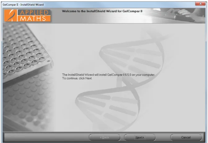
During a first-time installation of GelCompar II, theWelcome dialog boxwill display the version number of GelCompar II that is included with the Setup package (see Figure1.1.1).

2.2Please verify that you are installing the correct version and click<Next>to continue.

If an instance of GelCompar II 6.1 or older is already installed, the update Welcome dialog boxwill be displayed. This dialog box shows the version number of the installed instance of GelCompar II and the new version. The wizard will offer the choice between the installation of a new GelCompar II instance (choose a new installation directory) or to upgrade the existing instance (choose same installation directory as older version).

If an instance of GelCompar II 6.5 is already installed, theExisting Installed Instances Detected dialog box will appear when launching the Setup executable. This dialog box allows you to choose between installing a new GelCompar II instance or changing an existing instance.

(10)

6 1.1. Getting started

Figure 1.1.1:TheWelcome dialog box.

The next dialog will display the Software End User License Agreement (EULA).

2.3Please read the EULA carefully and click the topI accept the terms of the license agreement radio button

and the<Next>button to continue the installation.

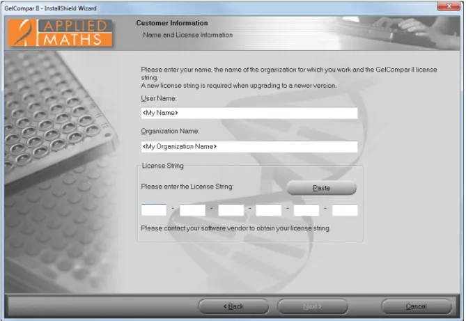
The user name, organization name and GelCompar II license string need to be entered in the Customer Information dialog box(see Figure1.1.2). The license string is provided on the sleeve of the CD–ROM or in case of an upgrade or an internet evaluation license, you may have obtained it electronically.

2.4Specify the user and organization names, enter the license string and press<Next>.

You must enter a valid license string to be able to continue with the installation. In addition the user and organization names cannot be empty.

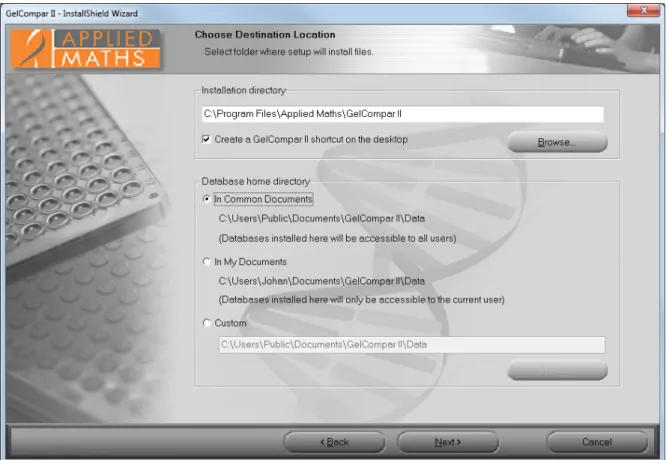
The installation directory for the GelCompar II application and the database home directory can be entered in theChoose Destination Location dialog box(see Figure1.1.3).

2.5Make sure the correct folders are specified and press<Next>once more.

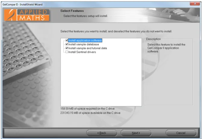
The GelCompar II features that you want to install on the local computer can be selected in the Select Features dialog box(see Figure1.1.4). Clicking on a feature in the left pane will display a short description in the right pane.

Install application software:

• In case of a standalone license, the Application software needs to be installed on each computer that you want to use to run the software. Please note that only on the computer where the dongle is attached to, you will be able to work with the software.

(11)

1.1.2. Software installation 7

Figure 1.1.2:TheCustomer Information dialog box.

you want to use to run the software. Please note that a permanent and stable internet connection is required to run the internet license.

• In case of anetwork license, theApplication software needs to be installed on the computers in the network that you want to use to run the software.

Install sample database and Install sample and tutorial data:

• TheSample databaseandSample and tutorial datathat are contained in the Setup package are used in the Quick Guide and in the Manual to illustrate the features of the software. Selecting these features will install the Sample database andSample and tutorial data in the GelCompar II home directory that is specified in theChoose Destination Location dialog box(see Figure1.1.3).

Install Sentinel drivers:

• In case of astandalone license, theSentinel drivers need to be installed on each computer that you want to use to run the software.

• In case of an internet license, you only need an internet connection to run the software. Since no USB dongle is needed to run an internet license, theInstall Sentinel drivers option does not need to be checked.

• In case of a network license, the Sentinel drivers only need to be installed on the NetKey+ server computer in the network where the hardware security key will be connected to.

(12)

Figure 1.1.3:TheChoose Destination Location dialog box.

• TheNetKey+ server program feature will only be visible and available for installation if a network li-cense string has been entered in theCustomer Information dialog box(see Figure1.1.2). TheNetKey+ server programfeature must only be installed on the computer in the network where the hardware se-curity key will be connected to.

2.6Tick the appropriate check boxes for the features you want to install and press<Next>.

If a network license string was entered in the Customer Information dialog box (see Figure

1.1.2), and if the GelCompar II application feature was selected for installation (see Figure

1.1.4), theNetKey+ connection settings dialog boxwill pop up where theNetKey+ Server name

andServer port numberconnection parameters can be entered. 2.7Click<Install>to start the installation.

TheSetup Status dialog boxis displayed.

If a network license string has been entered in theCustomer Information dialog box(see Figure

1.1.2), and theNetKey+ server program feature was selected for installation (see Figure1.1.4), the Setup will ask if you want to run the NetKey+ Configuration tool. This tool allows you to install and subsequently start the NetKey+ service.

2.8Press<Finish>to close theInstallShield Wizard.

2.9Double-click on the shortcut on your desktop to open GelCompar II. Alternatively, open the start menu

and select GelCompar II underAll programs.

(13)

1.1.2. Software installation 9

Figure 1.1.4:TheSelect Features dialog box.

(14)

1.1.3 Quick Guide tutorial data

The data used in the first two Parts of the Quick Guide (DatabaseandExperiments) can be installed with the software (checkInstall sample and tutorial datain theSelect Features dialog box, see Figure1.1.4). Alterna-tively, the data can be downloaded from the Applied Maths website: go tohttp://www.applied-maths. com, selectDownload,Sample data, andGelCompar II Tutorial Data.

The ComparisonsandIdentification Parts use theDemoBase Connecteddatabase. This database can be installed with the application software (checkInstall sample databasein theSelect Features dialog box, see Figure1.1.4).

(15)

Chapter 1.2

Creating and setting up a new database

1.2.1 Creating a new database

A GelCompar II database is a collection of samples which are potentially comparable to each other. Al-though a single database can be organized into subsets, very large databases can be unwieldy, so it is prefer-able to maintain unrelated samples in separate databases. As an example, we will create a new database containing closely relatedE. colisamples.

1.1In the GelCompar II Startup screen (see Figure1.1.5), press the button to enter theNew database

wizard.

1.2SpecifyE. colias the new database name and press<Next>twice.

1.3Press<Finish>and press<Proceed>to set up the new database as a connected Access database.

1.4Press<Proceed>in thePlugin installation toolbox. Plugins will be installed later.

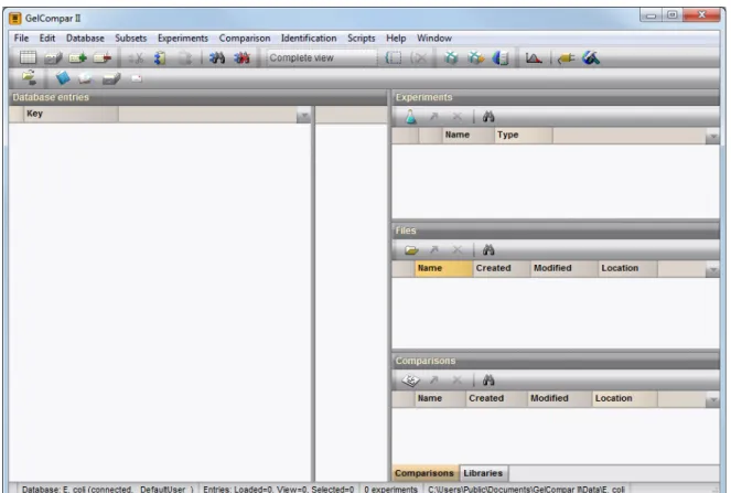
A new, empty database opens (see Figure1.2.1).

1.2.2 Setting up a new database

As an exercise, we will import data from the text file Ecoli-info.txt (see Figure 1.2.2) into our E. colidatabase. If theInstall sample and tutorial data feature was checked in theInstall wizard(see Figure

1.1.4), this text file can be found in theSample and Tutorial datafolder in the database home directory. Alternatively, this text file can be downloaded from our website: go tohttp://www.applied-maths.com, selectDownload,Sample data, andGelCompar II Tutorial Data.

2.1SelectFile>Importor press to call the Import tree.

2.2In the Import tree, expandEntry information data, highlightImport fields (text file)and press<Import>.

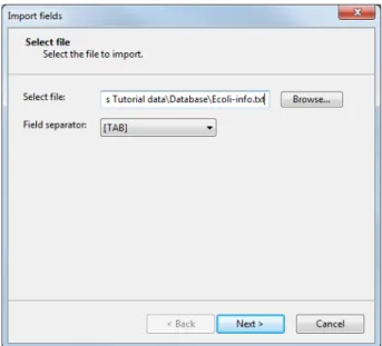
2.3In theSelect file step, browse for the Ecoli-info.txtfile in the GelCompar II Tutorial data

\Database folder. Select the file, select theTAB separator from the Field separator list and press

<Next>(see Figure1.2.3).

The way the entry information should be imported from the selected file into the database needs to be specified with an import template.

(16)

12 1.2. Creating and setting up a new database

Figure 1.2.1:TheGelCompar II main window.

Figure 1.2.2:Import entries from a text file.

This brings up a new dialog box (see Figure1.2.4). Each column in the selected file corresponds to a row in the grid (column 1 in the file corresponds to row 1 in the grid, column 2 corresponds to row 2, etc.). The text

File field is specified in theSource type column and the column names are displayed in theSourcecolumn. The last row in the grid holds the name of the file.

2.5Select the second row in the grid, press the<Edit destination>button and select the GelCompar IIKey

field from the list. Press<OK>. The grid is updated (see Figure1.2.4).

2.6Highlight the five other external fields in the grid panel using the Shift-key (make sure the last row in the

grid is not selected). Press the<Edit destination>button and select theEntry info field option from the

list. Press<OK>.

2.7Press<OK>once more to accept the default suggested names and press<Yes>.

(17)

1.2.2. Setting up a new database 13

Figure 1.2.3:Select the file to import and the separator.

Figure 1.2.4:Define a new import template.

2.8Optionally, change the default suggested templateNameand press<OK>.

The import template is added to the list and is automatically selected. 2.9Press<Next>twice.

(18)

(see Figure1.2.5).

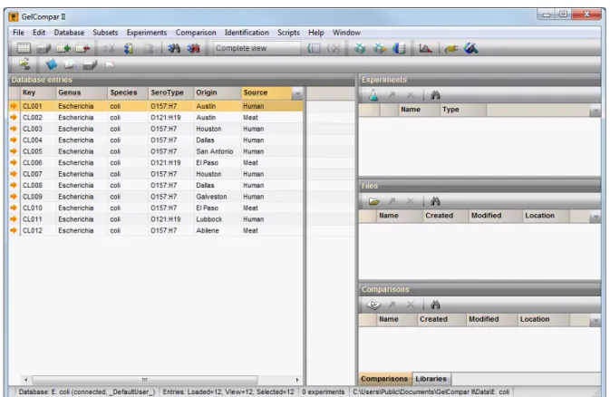
Figure 1.2.5:TheGelCompar II main windowafter import.

2.10Double-click on database entryCL001to open theEntry edit window.

Information can be edited in theEntry edit windowand saved (see Figure1.2.6).

Figure 1.2.6:TheEntry edit window.

2.11Close theEntry edit window.

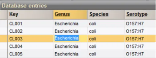
Alternative to using the Entry edit window, information in the information fields can be edited directly by clicking twice (not double-click) on an information field in the database. The information will appear highlighted and can be edited.

2.12Click twice on one of the information fields (not aKeyinformation field) or selectCtrl+Enter.

The information appears selected blue against a bright colored background and can be modified (see Figure

(19)

1.2.3. Selections of entries 15

Figure 1.2.7:Clicking twice on an information field enables direct editing.

2.13Use theArrowUpandArrowDown–keys on the keyboard to jump to the previous/next row.

2.14To jump to the next column, use theTab–key.

2.15To jump to the previous column, selectShift+Tabon the keyboard.

1.2.3 Selections of entries

1.2.3.1 Manual selections

3.1To select an entry in the database, hold theCtrl–key and click on the entry in theDatabase entries panel.

Alternatively, use the space bar to select entries.

The selected entry is marked by a colored arrow (see Figure1.2.8).

Figure 1.2.8:A selected entry.

3.2Selected entries are unselected in the same way (Ctrl+click).

3.3In order to select a group of entries, click on an entry, hold theShift–key and click on another entry.

All entries that are listed between these two entries are selected, including the two entries.

3.4To select all entries in the database, useEdit>Select all entries(Ctrl+A).

3.5To clear a selection in the database, useEdit>Unselect all entries( ,F4).

1.2.3.2 Automatic search and select functions

Simple and intuitive search functions can be used to search and select entries.

3.6SelectEdit>Search entries... ( ,F3).

3.7In theEntry search window, enter for example ”Dallas” in theOriginfield (see Figure1.2.9) and press

<Search>.

All entries having the name ”Dallas” in their ’Origin’ field are selected.

(20)

(21)

Part 2

(22)

(23)

Chapter 2.1

Fingerprint data

2.1.1 Introduction

In this Chapter we will:

• Create a fingerprint type experiment • Import a fingerprint gel image file • Process the fingerprint gel file • Link fingerprint data to entries

2.1.2 Sample data

As an exercise, we will import a 8-bit TIFF gel image which was generated by PFGE with the restriction en-zymeXba-Iin ourE. colidatabase. The gel image can be downloaded from the Applied Maths website: go tohttp://www.applied-maths.com, selectDownload,Sample data, andGelCompar II Tutorial Data. If theInstall sample and tutorial data feature was checked in theInstall wizard(see Figure1.1.4), the gel image can be found in theSample and Tutorial datafolder in the database home directory.

2.1.3 Create a fingerprint type experiment

First we need to create a new fingerprint type experiment before we can import a gel image file in ourE. colidatabase.

3.1In the GelCompar II startup screen, double-click on theE. colidatabase – created in1.2.1– to open it.

3.2In theGelCompar II main window, selectExperiments >Create new fingerprint type from the main

menu, or press the button from theExperiments panel toolbarand selectNew fingerprint type.

3.3Enter a name, for examplePFGE-XbaIand press<Next>.

3.4In the next window, selectTwo–dimensional TIFF files and8–bit OD depth (256 gray values). Press

<Next>to proceed.

(24)

20 2.1. Fingerprint data

3.6Press<Next>to proceed.

3.7In the final step, leaveNoselected for applying a background subtraction.

3.8Press<Finish>.

TheExperiments panelnow lists the fingerprint typePFGE–XbaI(see Figure2.1.1).

Figure 2.1.1:TheExperiments panel.

You can still change the resolution, inversion, and background subtraction settings later when processing a gel.

2.1.4 Import a fingerprint gel image file

4.1SelectFile>Add new experiment file...( ) in theGelCompar II main window.

4.2Select the fileec-XbaI-001.tifin theGelCompar II Tutorial data\PFGE TIFFSfolder.

A box appears asking if you want to edit the image. Press<No>if you are sure the file is an uncompressed gray scale TIFF image. For the conversion to an uncompressed gray scale TIFF file press<Yes>.

4.3Since the example file is an uncompressed gray scale TIFF file, press<No>.

The gel image is now available in theFiles panel(see Figure2.1.2). The file is marked with a red ”N” ( ) indicating that the image has not been processed yet.

Figure 2.1.2:TheExperiments panelandFiles panel.

2.1.5 Process the fingerprint gel file

Before linking our fingerprint lanes to entries in our database, we must define and process the lanes in the Fingerprint data window.

(25)

2.1.5. Process the fingerprint gel file 21

5.2In theFingerprint file window, selectFile>Edit fingerprint datato open theFingerprint data window.

5.3In the next dialog box, selectPFGE-XbaIand press<OK>.

TheFingerprint data windowopens and the imported gel image is surrounded by a green rectangle. Since GelCompar II recognizes the darkness as the intensity of a band, make sure the bands appear as dark bands on a white background (see Figure2.1.3).

In case the bands appear as white bands on a black background, invert the values: press to open theFingerprint conversion settings window, check/uncheck theInverted valuescheck box, and press<OK>to apply the changes.

2.1.5.1 Define strips

The first step in processing a gel is to crop the image to remove empty space, and to define the lanes.

5.4Delineate the area of the gel lanes by clicking and dragging the nodes of the rectangle to adjust it. Exclude

the wells from the rectangle (see Figure2.1.3).

Figure 2.1.3:Area of gel lanes.

5.5In the toolbar, press to let the software search for the individual lanes.

5.6Enter ”10” as the approximate number of lanes and press<OK>.

5.7In the toolbar, press to open theFingerprint conversion settings window.

When opened in theStrips paneltheRaw data tabis selected by default.

5.8Adjust theThicknessof the image strips so the splines border the edges of the bands (e.g.33points).

5.9Press<OK>.

5.10Adjust the horizontal position of each spline as necessary by clicking and dragging a blue node. Hold

(26)

5.11Decrease the thickness of the spline in lane10by clicking one of its nodes and repeatedly pressing or

F8. Then move the spline over to the good portion of the lane to the left (see Figure2.1.4).

Figure 2.1.4:Adjusting the thickness and positions of the splines.

Next, we will edit the tone curve to improve the band visibility.

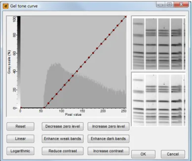
5.12From the pull down menu, selectEdit>Edit tone curve.

5.13Press<Linear>. The visible gray scale interval now ranges between the minimum and maximum values

in the image (see Figure2.1.5).

Figure 2.1.5:TheGel tone curve window.

5.14Press the other editing buttons such as<Enhance weak bands>a few times until you have a clear and

sharp image.

5.15Press<OK>to save changes to the tone curve settings.

The gel tone curve does not change the image’s densitometric values, only the way they appear in theFingerprint data window.

5.16Press to save the work already done.

(27)

2.1.5. Process the fingerprint gel file 23 2.1.5.2 Define curves

Now that the lanes have been defined, the software can generate densitometric curves describing the optical density across the spline along each lane. The left panel shows the strips extracted from the image file, the right panel shows the densitometric curve of the selected pattern (see Figure2.1.6). The area between the blue lines of each lane will be used to calculate the densitometric curve.

5.18Select lane3.

Near the top of the lane in the spline there is a pinpoint spot. As a result, a thin peak appears on the densitometric curve shown on the right side of the window.

5.19It might help to zoom in on the image using the zoom slider.

5.20Open theFingerprint conversion settings windowagain (click on the button).

5.21Change theAveraging thicknessfor curve extraction to15in theDensitometric curves tab.

5.22CheckMedian filterand press<OK>.

In lane 3, the thin peak – resulting from the pinpoint spot – has disappeared in the densitometric curve shown on the right side of the window (see Figure2.1.6).

Figure 2.1.6:Increased splines and median filtering.

GelCompar II can analyze the gel image to determine the optimal settings for removing background noise from the densitometric curves.

5.23SelectCurves>Spectral analysis.

The following settings are shown in theSpectral analysis window:

1. Wiener cutoff scale: Determines the optimal setting for least square filtering. 2. Background scale: Estimation of the disk size for background subtraction.

(28)

5.24Close theSpectral analysis window.

5.25Open theFingerprint conversion settings windowagain (click on the button).

5.26CheckApply least square filteringand specify aLeast square filtering Cut off as indicated by the Wiener

cutoff scale in the Spectral analysis window(use the percentage value, e.g.1). Least square filtering

removes very small peaks from the curves.

5.27Check Apply in theBackground subtraction panel and specify aBackground subtraction disk size as

indicated by the background scale in theSpectral analysis window(use the percentage value, e.g.14).

Background subtraction removes large background trends from the curves. 5.28Press<OK>.

The background noise has been removed from the curves (see Figure2.1.7).

Figure 2.1.7:Curves after filtering.

5.29Press to save the work already done.

5.30Press to proceed to theNormalizationstep or press theNormalization tab.

2.1.5.3 Normalize the gel

Every fingerprint type experiment needs at least one reference system to normalize its gels. Since this is the first Xba-I gel we have imported, we need to create a reference system based on the standard pattern in this gel. We will use the standard’s molecular weights to name the reference positions. Subsequent Xba-I gels, provided they contain the same standard, will be normalized with the same reference system.

5.31Press to enter the normalized view.

For now, the ”normalized view” looks the same as the original view. In a first step we will define the reference lanes and the reference bands.

5.32Select lane1and press to assign it as a reference lane or selectReferences >Use as reference lane.

5.33Repeat this for lane6and lane10.

5.34Choose the most suitable standard lane for creating the reference system. For this exercise select lane6

(29)

5.35Right-click on the top band in lane6and selectReferences>Add external reference positionfrom the

pop-up menu.

5.36Enter582.6and press<OK>.

5.37Repeat the process for each band in lane6as shown in Figure2.1.8.

Figure 2.1.8:Reference system.

The reference system for experiment typePFGE-XbaIis now defined (see Figure2.1.9).

5.38SelectNormalization>Auto assignor press .

5.39Make sureUsing bandsis selected and press<OK>.

5.40Carefully inspect the assignments made (see Figure2.1.9).

5.41If a band assignment is incorrect, select the band and press theDel–key.

5.42To assign a reference band manually, first click on the reference position tag, then hold theCtrl–key and

click on the reference band to assign it to that reference position.

5.43To update the normalization based on the band assignments, selectNormalization>Update

normaliza-tionor press .

5.44Press to proceed to the last step. Alternatively press theBands tab.

2.1.5.4 Define bands

If you want to use the curves to compare the patterns, no bands need to be assigned and this last step can be skipped. If you want to compare the patterns using bands, you will need to assign bands in the sample lanes

(30)

Figure 2.1.9:Reference positions assigned.

in this last step. Usually, assigning bands in the sample lanes is done first with the software’s automatic band search, followed by manual corrections. Some trial and error might be required to find the best settings for the automatic band search.

5.45To automatically search for bands, press or selectBands>Auto search bands.

In theBand search window, the currently selected lane is shown along the bottom (see Figure2.1.10).

(31)

5.46To scroll through other lanes, press the<and>buttons on the left and right sides of the curve.

5.47Enter5forMin. Profiling,2forGray zone, and press<Preview>.

The red lines across the lane at the bottom of the window indicate which peaks will be assigned bands with the current settings. The purple area along the curve indicates the minimum profile above which a band is assigned, while the blue area indicates the gray zone in which bands are considered ”uncertain”.

5.48Press<Search on all lanes>to execute the band search with these settings.

Bands that are found are marked with a green horizontal line, whereas uncertain bands are marked with a small green ellipse (see Figure 2.1.11). If you see any incorrect band assignments you can edit them manually:

• To add a band, hold down theCtrl–key and click on the spot. The cursor automatically jumps to the closest peak; to prevent this, hold down theTab–key while clicking.

• To select a group of bands, hold down the Shift–key and click while dragging the mouse pointer diagonally across the bands.

• To delete one or more selected bands, press theDel–key.

• To mark a band as uncertain, click on the band and selectBands>Mark band(s) as uncertainor press F5. To mark a band as certain, click on the band and selectBands>Mark band(s) as certain or press F6.

5.49After you are satisfied with the band assignments, press to save the file.

Figure 2.1.11:TheBands tab.

5.50The program may prompt with the following question: ”The resolution of this gel differs considerably

from the normalized track resolution. Do you wish to update the normalized track resolution?” If the question appears, answer<Yes>.

(32)

5.51Exit theFingerprint data windowby selectingFile>Exit.

5.52The software asks: ”Settings have been changed. Do you want to use the current settings as new

de-faults?” Select<Yes>so that the settings used for this gel will be saved in the fingerprint type settings.

Congratulations! You have processed your first gel. The reference system and fingerprint settings that are saved with the fingerprint type experiment will make future XbaI gels much faster to process.

2.1.6 Link fingerprint data to entries

Although we have created individual fingerprint lanes from our gel image, the software does not know which lanes correspond to which entries in the database. Our next task is to link the fingerprint lanes to the entries in our database.

6.1In theFiles panel, double–click on the filenameec-XbaI-001to open theFingerprint file window(see

Figure2.1.12).

6.2Select lane2and selectDatabase>Link laneor press .

6.3In the dialog box enterCL004and press<OK>.

You can also link a lane to a database entry by dragging the gray arrow icon to the entry key in the database window. When a lane is linked, the icon becomes purple: .

6.4Drag the arrow icon of lane3to entryCL001.

6.5Continue linking the remaining non–reference lanes fromec-XbaI-001to the appropriate database entries

as shown in Figure2.1.12.

Figure 2.1.12:Fingerprint file with linked lanes.

6.6After linkage, close theFingerprint file windowand open the gel strip for one of the entries in the database

by clicking on a colored dot in theExperiment presence panel.

The card is displayed in raw mode (i.e. not normalized). The band sizes are shown as relative distances from the top (see Figure2.1.13).

(33)

2.1.7. Fingerprint type experiment settings 29

Figure 2.1.13:Fingerprint type experiment card: raw mode.

6.7Close the card by clicking in the small triangle–shaped button in the upper left corner.

2.1.7 Fingerprint type experiment settings

2.1.7.1 Assigning a standard pattern

7.1Open the fingerprint experiment typePFGE-XbaI by double–clicking on the experiment type in the

Experiments panel.

TheFingerprint type windowshows the defined reference positions in relation to the distance on the pattern in percentage. The reference system is calledR01. The panel left from the reference system is still blank: the fingerprint still misses a standard pattern. We will link aStandardpattern (e.g. lane6ofec-XbaI-001, i.e. the one used for defining the reference system) to thePFGE-XbaIfingerprint type as follows:

7.2Close theFingerprint type window.

7.3In theFiles panel, double–click onec-XbaI-001to open theFingerprint file window.

7.4In theFingerprint file window, add lane6to the database by selecting it and pressing .

7.5In the dialog box, enter ”REF” and press<OK>.

7.6Select<Yes>to create the new entry in the database.

A new entryREFis created with the pattern from lane6ofec-XbaI-001linked to it.

7.7Close theFingerprint file window.

7.8Open the fingerprint experiment typePFGE-XbaI by double–clicking on the experiment type in the

Experiments panel.

7.9Press next toStandardin theSettings paneland drag it over to theREFdatabase entry.

The standard pattern is now displayed in the panel next to the reference positions, and the database entry keyREFis indicated as theStandard(see Figure2.1.14).

If a standard pattern is assigned to a fingerprint type, this standard pattern is shown in theNormalization tabof theFingerprint data window(see Figure2.1.9) to make visual assignment of bands to the reference positions easier. The choice of a standard has no influence on the normalization process since it is only used as visual aid.

(34)

Figure 2.1.14:TheFingerprint type window. 2.1.7.2 Calculating a calibration curve

One more step is necessary before we can analyze our fingerprint patterns. Since there are gaps present between the reference system positions, we must tell the software how to convert other band positions into metrics (e.g. molecular weights). We will use the reference system to construct a calibration curve which translates all band positions into metrics.

7.10In theFingerprint type window, selectSettings>Edit reference systemor double-click onR01.

TheReference system windowappears with the message: ”Could not calculate calibration curve. Not enough markers.”

7.11Since the molecular weights were already entered as names for the reference positions, we can copy these

molecular weights by selectingMetrics>Copy markers from reference system. Confirm the action.

7.12Designate a metric unit withMetrics>Assign units, enterkband press<OK>.

7.13Close theReference system window, and close theFingerprint type window.

The fingerprint typePFGE-XbaIis now defined and configured, and one gel has been added to the database.

7.14Open a gel strip for one of the entries in the database by clicking on a colored dot in the Experiment

presence panel.

The cards are now displayed in normalized mode (see Figure2.1.16). Band sizes are shown as molecular sizes based on the regression curve calculated in the previous step.

7.15Increase or decrease the size of the card using the keyboard by pressing the numerical ”+” key (increase)

or the numerical ”-” key (decrease).

(35)

2.1.8. Additional practice 31

Figure 2.1.15:Calibration curve calculated.

Figure 2.1.16:Fingerprint type experiment card: normalized mode.

2.1.8 Additional practice

2.1.8.1 XbaI-002

A second gel file,ec-XbaI-002.tif, which was generated by PFGE with the restriction enzymeXba-Iis present in theGelCompar II Tutorial data\PFGE TIFFSfolder. For this second PFGE-XbaI gel, we will use the same fingerprint type, reference system, and conversion settings used for the first gel.

8.1Add and process gelec-XbaI-002.tif(see Instruction4.1 in chapter 2.1to Instruction5.52 in chapter

2.1). Use lanes1,4,7, and10as the reference lanes. The reference system defined for the first gel is

displayed in theNormalization tab. In theNormalization tab, you will just have to select the reference

lanes, and let the software look for the reference bands based on the reference system (Instruction5.34 in

chapter 2.1to Instruction5.37 in chapter 2.1can be skipped).

8.2After processing the gel, link the lanes to the appropriate database entries (see Figure2.1.17).

8.3When linking lane6to entry with keyCL010, GelCompar II will ask whether or not you want to create

a duplicate key for this entry.

(36)

Figure 2.1.17:Linking the lanes for gel ec-XbaI-002 to the database entries.

2.1.8.2 AvrII-001

A second set of gels is present in theGelCompar II Tutorial data\PFGE TIFFSfolder. These gels are created with the restriction enzymeAvr-II. To import these gels in the database, another fingerprint type experiment is needed.

8.5Create a new fingerprint type experiment calledPFGE-AvrII, using the same settings as PFGE-XbaI (see

Instruction3.2 in chapter 2.1to Instruction3.8 in chapter 2.1).

8.6Process the AvrII gelec-AvrII-001.tif, using lanes1,6, and10as the reference lanes. Be sure to

selectPFGE–AvrIIas the fingerprint type when opening the file for the first time.

The reference system used in the gels XbaI-001 and XbaI-002 is the same as used in gel AvrII-001.

8.7To facilitate the assignment of reference positions in gel AvrII-001, selectReferences >Copy

normal-ization in step 3 of one of the XbaI gels and then selectReferences >Paste normalization in step 3 of the AvrII-001 gel. The reference positions will be transferred from the XbaI gel to the AvrII gel.

8.8SelectNormalization>Auto assignor press .

8.9Make sure thatUsing bandsis selected and press<OK>. Reassign the bands if needed.

After processing the gel, link the lanes to the appropriate database entries as shown in Figure2.1.18.

8.10Open the fingerprint type experiment PFGE-AvrIIby double–clicking on the experiment type in the

Experiments panel.

8.11Press next toStandardin theSettings paneland drag it over to theREFdatabase entry.

8.12In the same window, selectSettings>Edit reference system and selectMetrics >Copy markers from

reference system. Confirm the action.

8.13Designate a metric unit withMetrics>Assign units, and enterkb. Press<OK>.

(37)

Figure 2.1.18:Linking the lanes for gel ec-AvrII-001 to the database entries.

2.1.8.3 AvrII-002

Process the second PFGE-AvrII gel,ec-AvrII-002.tif, using lanes1,4,7, and10as the reference lanes. Link the lanes to the database entries as you did for XbaI-002 (see Figure2.1.17).

(38)

(39)

Part 3

(40)

(41)

Chapter 3.1

General comparison functions

3.1.1 Comparison settings

If the Install sample database feature was checked in theInstall wizard (see Figure 1.1.4), the database DemoBase Connectedshould be listed in the GelCompar II Startup screen.

1.1In the GelCompar II Startup screen, double-click onDemoBase Connectedto open it.

1.2To view the comparison settings for an experiment in the database (e.g.RFLP2) double–click on the

experiment in theExperiments panel.

The comparison settings are shown in theComparison settings panel.

1.3SelectSettings>Comparison settings to open theComparison settings window.

1.4Change the settings if desired and close theComparison settings window.

1.5Close theExperiment type window.

3.1.2 Compare two entries

A pairwise comparison is useful because it shows every detail of the comparison for each experiment. For example, if you want to know exactly how the bands from two fingerprints are aligned, a pairwise comparison will show the alignment.

2.1In the GelCompar II startup screen, double-click onDemoBase Connectedto open it. In case the

De-moBase Connectedwas already open, clear any previous selection by pressingF4.

2.2Select any two entries you want to compare (except STANDARD). Use the Ctrl-button to select the

entries.

2.3SelectComparison>Compare two entriesor pressCtrl+Alt+C.

In thePairwise comparison window, all experiments present in the database are listed in theExperiments panel. The similarity values are shown in theSimilarity column (see Figure3.1.1).

2.4Select an experiment in the left panel to display the comparison details in the right panel.

(42)

38 3.1. General comparison functions

Figure 3.1.1:ThePairwise comparison window.

3.1.3 Create a new comparison

To compare more than two entries, theComparison windowis used.

3.1Clear any previous selection by pressingF4.

3.2SelectEdit>Search entries...( ,F3).

3.3Specify the nameSTANDARDin theGenus text box, selectNegative search and press the<Search>

button (see Figure3.1.2).

Figure 3.1.2:TheEntry search window. All non–STANDARD entries are selected in the database.

3.4SelectComparison >Create new comparison (Alt+C) or press the button from theComparisons

(43)

3.1.4. Comparison window 39 AComparison windowis created with the selected database entries.

3.1.4 Comparison window

4.1Drag the separator lines between the panels in theComparison windowto the left or right to size them

optimally.

4.2Drag the separator lines between the field names in theInformation fields panelto the left or right to size

the columns optimally.

The Comparison windowshows the database entries in theInformation fields paneland the images of the experiments in the Experiment data panel. TheExperiments panellist the experiment types, the Groups panellists the group sizes and names, and theAnalyses paneldisplays the analyses. The other two panels contain the dendrogram (Dendrogram panel) and similarity matrix (Similarities panel), if calculated.

3.1.4.1 Comparison layout

Each experiment type in theExperiments panelcontains two objects: a button and the experiment type name on the right hand side of the button. For a fingerprint type, the button is shown as and for a composite data set as .

4.3Press next toRFLP1. The fingerprints forRFLP1are shown in theExperiment data panel(see Figure

3.1.3).

When the experiments are shown, the icon is displayed with a green check.

4.4Press next toRFLP2. TheRFLP2data are shown to the right ofRFLP1(see Figure3.1.3).

Figure 3.1.3:TheComparison window: Two fingerprint types are shown.

4.5If there is not enough space to show both images at the same time, scroll through the data panel, or use

(44)

40 3.1. General comparison functions

4.6Drag the separator line between the experiments to the left or to the right to adjust the horizontal space

for a particular experiment.

4.7Select experiment typeRFLP1in theComparison windowby selecting its name in theExperiments panel

or click on the RFLP1 image in theExperiment data panel(if shown).

Functions like clustering, PCA, and band matching, as well as layout functions, apply to the currently se-lected experiment type. When performing any of these functions, be sure the correct experiment is sese-lected!

3.1.4.2 Add and remove entries

4.8Unselect all entries by pressing theF4key.

4.9Select a few entries in theInformation fields panelof theComparison window(use theCtrlandShift–

keys to select/unselect entries).

4.10Press and confirm the action. The selected entries are removed from the comparison.

4.11Press . The selected entries are pasted back into the comparison at the position of the selection bar.

4.12SelectFile>Save( ,Ctrl+S) to save the comparison and enter ”All” as the name. Press<OK>.

4.13SelectFile>Exitto close the comparison.

ComparisonAllis now listed in theComparisons panelof theGelCompar II main window.

3.1.4.3 Create groups

An important display function in theComparison windowis the creation of groups. Groups are subsets of comparison entries that can be defined from clusters, from database fields, or from any subdivision the user desires.

As an example we will use theGenusdatabase field to assign groups in our comparison.

4.14In theDemoBase Connecteddatabase, double–click on the comparisonAllin theComparisons panelof

theGelCompar II main windowto open theComparison window. The comparisonAllcontains all non–STANDARD entries (see3.1.3).

4.15Press the F4key to clear any selected entries. Right–click on the database field name Genusin the

Information fields paneland selectCreate groups from database field.

4.16Select the order in which groups are created (i.e. by size, alphabetically, or by position in the comparison)

and press<OK>to create the groups.

Every genus is now assigned to a unique group. They appear in theGroups panelalong with their sizes and names (see Figure3.1.4).

(45)

3.1.4. Comparison window 41

(46)

(47)

Chapter 3.2

Clustering fingerprint data

3.2.1 Comparison window

1.1In theDemoBase Connecteddatabase, double-click on the comparisonAllin theComparisons panelof

theGelCompar II main windowto open theComparison window. The comparisonAllcontains all non-STANDARD entries (see3.1.3).

1.2Press next toRFLP1. The fingerprints forRFLP1are shown in theExperiment data panel(see Figure

3.1.3).

1.3SelectFingerprints>Settings>Show metrics scale( ) to display the metric (e.g. molecular weight)

scale of the selected fingerprint type.

1.4Press to show the band positions in theExperiment data panel.

3.2.2 Cluster fingerprint data

Cluster analysis is a two-step process. First, all pairwise similarity values are calculated with asimilarity coefficient. Then, the resulting similarity matrix is converted into a dendrogram with a clustering algo-rithm. Although in practice these steps are performed together, they each require their own comparison settings.

2.1SelectClustering >Calculate >Cluster analysis (similarity matrix) or press and selectCalculate

cluster analysis.

The Comparison settings wizardallows you to specify the settings related to the similarity coefficient for calculation of the similarity matrix and the clustering method to be applied. The first step deals with the similarity coefficient (see Figure3.2.1).

2.2SelectDicefrom the list.

Additional settings are listed in the right panel.

2.3Enter aOptimizationof 0.50%, and aBand matching Toleranceof 0.50%. Leave all the other settings to

0% (see Figure3.2.1).

TheOptimizationsetting limits the amount of movement for each fingerprint as a whole. TheBand matching Tolerance settinglimits the amount of movement for each band.

(48)

44 3.2. Clustering fingerprint data

Figure 3.2.1:Select similarity coefficient.

In step 2 of the Comparison settings wizard, the options related to the clustering algorithms are grouped (see Figure 3.2.2). Under Method, the clustering algorithm to be applied on the similarity matrix can be selected. ADendrogram name can be entered in the corresponding text box. By default, the name of the experiment type will be used.

2.5SelectUPGMA, checkCalculate error flagsand selectCophenetic correlationfrom theBranch quality

list (see Figure3.2.2).

IfCalculate error flagsis checked, the program will calculate the standard deviations associated with each cluster. TheCophenetic Correlation is another parameter that expresses the consistency of a cluster. This method calculates the correlation between the dendrogram-derived similarities and the matrix similarities. The value is calculated for each cluster thus estimating the faithfulness of each sub-cluster of the dendro-gram.

2.6Press<Next>again in theComparison settings wizardto start the cluster analysis.

During the calculations, the program shows the progress in theComparison window’s caption (as a percent-age), and there is a green progress bar in the bottom of the window.

When finished, the dendrogram and the similarity matrix are displayed in their corresponding panels. The cluster analysis is listed in theAnalyses panelof theComparison window(see Figure3.2.3).

TheCophenetic correlationis shown at each branch, together with a colored dot, of which the color ranges between green-yellow-orange-red according to decreasing cophenetic correlation. This makes it easy to detect reliable and unreliable clusters at a glance.

Blue bars are also shown at each node, corresponding to theStandard deviation of values in that region of the similarity matrix. The average and the standard deviation of similarity values for the selected node are

(49)

3.2.2. Cluster fingerprint data 45

Figure 3.2.2:Select clustering algorithm.

Figure 3.2.3:TheComparison window. shown above the dendrogram.

2.7Left-click on the dendrogram to place the cursor on any node or tip (where a branch ends in an individual

(50)

46 3.2. Clustering fingerprint data

2.8To select entries in a cluster, click on the node of the cluster while holding the Ctrl-button.

2.9Press to remove the selected entries from the cluster analysis. Confirm the action. The dendrogram is

automatically updated.

2.10SelectEdit>Paste selectionor . The cluster analysis is recalculated automatically, and the selected

entries are placed back in the dendrogram.

A branch can be moved up or down to improve the layout of a dendrogram:

2.11Click the branch which you want to move up in the dendrogram and selectClustering>Move branch up

or press the button in theDendrogram panel.

2.12Click the branch which you want to move down in the dendrogram and selectClustering>Move branch

downor press the button in theDendrogram panel.

To simplify the representation of large and complex dendrograms, it is possible to simplify branches by abridging them as a triangle.

2.13Select a cluster of closely related entries and selectClustering>Collapse/expand branch or press the

button in theDendrogram panel. Repeat this action to undo the abridge operation.

2.14If no groups are defined in theComparison window, right-click on the field nameGenusin the

Informa-tion fields panel, selectCreate groups from database fieldand confirm.

2.15SelectClustering>Dendrogram display settingsor press the button in theDendrogram panel.

This pops up theDendrogram display settings dialog box.

2.16UncheckShow error flags, uncheckShow branch quality, and enableShow group colors. Press<OK>.

The dendrogram branches are now colored according to the group colors (see Figure3.2.4).

2.17SelectClustering >Show information or press in theDendrogram panel. This pops up aReport

windowwith the comparison settings. Close theReport window.

2.18Save the comparison with the dendrogram by selectingFile>Saveor pressing .

3.2.3 Matrix display functions

The similarity values in theSimilarities panelare represented by shades of blue.

3.1To show the values in the matrix, select in the toolbar of theSimilarities panel.

3.2To view a pairwise comparison, double-click on the appropriate cell in the matrix.

3.2.4 Print a cluster analysis

GelCompar II can export the cluster analysis as it appears in theComparison window.

4.1SelectFile>Print preview.

4.2To scan through the pages that will be printed out, press and , or use thePageUpandPageDown

keys.

(51)

Figure 3.2.4:Show group colors on dendrogram.

4.4To enlarge or reduce the whole image, press or .

4.5If a similarity matrix is available, it can be included by pressing the button.

4.6On top of the page, there are a number of small yellow slide bars, which can be moved.

4.7To preview and print the image in full color selectLayout >Use colors or press .

4.8Export the image to the clipboard by pressing and selecting an appropriate format.

4.9If a printer is available, press or to print one or all pages.

4.10SelectFile>Exitto close theComparison print preview window.

3.2.5 Additional practice

5.1In theE. colidatabase - created in1.2.1- create a comparison of all the database entries exceptREF.

5.2Create groups from theSourcedatabase field.

(52)

(53)

Chapter 3.3

Band matching tables

3.3.1 Create a band matching table

Fingerprint patterns do not have well-defined characters. Band positions vary continuously, although they do tend to fall into categories, or band classes. GelCompar II allows you to formally define band posi-tion classes, thereby creating a band matching table. This in turn allows you to apply more sophisticated analytical tools, such as polymorphism analysis and principal components analysis.

3.3.1.1 Create a composite data set

As will be described in the next Chapter, a composite data set can be used to combine two or more experi-ments. A composite data set can also be used to convert fingerprint band classes into a band matching table. As an exercise we will define a composite data set containing the fingerprint experimentRFLP1.

1.1In theDemoBase Connected database, press from theExperiments panel toolbarand selectNew

composite data set.

1.2EnterRFLP1-tableand press<OK>.

Figure 3.3.1:TheComposite data set window.

(54)

50 3.3. Band matching tables

TheRFLP1experiment is checked with a green V-sign (see Figure3.3.1).

1.4Close theComposite data set window.

RFLP1-tableis shown in theExperiments panelof theGelCompar II main window(see Figure3.3.2).

Figure 3.3.2:TheExperiments panel. 3.3.1.2 Create band classes

Band classes are position categories to which individual bands are assigned. Just as the position tolerance and optimization settings determine how a pair of fingerprint patterns are aligned, they also determine how band classes are created for a whole comparison. The result is a band table with defined columns corre-sponding to band class positions.

1.6In theComparison window, selectRFLP1in theExperiments paneland press .

1.7SelectFingerprints>Perform band matchingor press the button.

1.8SelectFind classes on all entriesand press<OK>.

The software defines the band classes forRFLP1and assigns each band to a class. The classes are shown as blue lines (see Figure3.3.3).

1.9Use the zoom sliders to obtain the best view of the band classes.

All band classes are labeled with a band class label. If a band class is selected, its label is highlighted. If a regression curve is calculated for the reference system, the metric positions of the band classes are displayed in the label.

3.3.1.3 Display the band matching table

The band classes are shown as blue lines crossing the fingerprints. To analyze them further, the band classes must be displayed as a band table, using a composite data set.

1.10Show the band matching table by pressing next toRFLP1-table.

Each cell in the table represents a band’s presence or absence.

1.11To see the band class labels completely, drag the separator line between the table and the labels

(55)

3.3.2. Band polymorphism analysis 51

Figure 3.3.3:Band classes.

1.12To export a tab-delimited text file containing the binary band matching table, selectComposite>Export

character tableand press<Yes>.

1.13To show the intensity of the bands as colors, chooseComposite>Show quantification (colors)( ) (see

Figure3.3.4).

1.14To display the intensities of the bands as numerical values, selectComposite >Show quantification

(values).

Figure 3.3.4:Left: band classes on the fingerprint type; Right: intensities of the bands shown in color.

3.3.2 Band polymorphism analysis

Band matching tables allow you to identify band classes that discriminate sets of entries. For example, you might want to identify bands that appear only in certain entries. Such discriminating bands can then be analyzed further using other experimental methods.

(56)

52 3.3. Band matching tables

3.3.2.1 Find discriminative band classes

Band classes can be sorted based on how well they discriminate a set of entries from the rest. In this example we will find band classes that separateVercingetorixentries from the others.

2.1Make sure the composite data setRFLP1-tableis shown and selected in theComparison window.

2.2Minimize or reduce theComparison windowso that theInformation fields window(at least the menu and

toolbar) becomes visible.

2.3PressF4to make sure that no entries are selected.

2.4PressF3and enterV*in theGenusfield of theEntry search window. Press<Search>.

2.5To view the selected entries, chooseEdit>Arrange entries>Bring selected entries to topin the

Com-parison window.

2.6SelectComposite>Discriminative characters.

The characters (band classes) are rearranged so that the characters positivefor the selected entries are to theleft, and the charactersnegativefor the selected entries are to theright. Characters in the middle are relatively uninformative with respect to the delineation of Vercingetorix.

3.3.2.2 Sort entries by band intensity

The band matching table also allows you to sort entries by band intensity. This helps to identify entries for which a band of particular interest is present.

2.7SelectComposite>Show quantification (colors)( ) to show the band table as an intensity table.

2.8Select a band class by clicking on its label in the header. The band class is highlighted.

2.9SelectComposite>Sort by characteror press the button.

The entries are now sorted by increasing band intensity for the selected band class.

3.3.3 Additional practice

3.1In the E. colidatabase - created in 1.2.1- create a new composite data set for both fingerprint types

PFGE-XbaIandPFGE-AvrII.

(57)

Chapter 3.4

Composite data sets

3.4.1 Introduction

With a composite data set multiple experiments can be combined into a single analysis. Two options are possible for the calculation of the similarity between entries based on a composite data set:

• Option 1: The individual similarity matrices are calculated for each experiment type that is present in the composite data set, and a combined matrix is then calculated by averaging the values.

• Option 2: All characters from the different experiment types present in the composite data set are merged, and from this set, the similarity matrix is calculated (= ”combined matrix”).

3.4.2 Combine fingerprint experiments

In this example we will combine two fingerprint type experiments.

3.4.2.1 Create a composite data set

2.1In theDemoBase Connected database, press from theExperiments panel toolbarand selectNew

composite data set.

2.2Enter a name (e.g.”RFLP–combined”) and press<OK>.

TheComposite data set windowis shown forRFLP-combined(see Figure3.4.1).

2.3SelectRFLP1and selectExperiment>Use in composite data set.

When an experiment type is selected in the composite data set, it is marked with a green check.

2.4Repeat this forRFLP2.

2.5SelectFile>Exitto close the window.

(58)

54 3.4. Composite data sets

Figure 3.4.1:TheComposite data set window. 3.4.2.2 Cluster analysis of a composite data set

Option 1: Average the individual matrices

2.7SelectRFLP-combinedin theExperiments paneland selectClustering>Calculate >Cluster analysis

(similarity matrix) or press and selectCalculate cluster analysis.

2.8Select the optionAverage from experimentsand press<Next>.

2.9Leave all settings unaltered in the next step of the wizard and press<Next>once more.

With the optionAverage from experiments, the similarity matrices from the individual experiments (RFLP1 andRFLP2) are averaged. The resulting dendrogram is based upon this average matrix.

Option 2: Create combined character matrix

Fingerprints can only be combined to a character matrix if a band matching is performed (see Chapter3.3).

2.11In theComparison window, selectRFLP1in theExperiments paneland press .

2.12SelectFingerprints>Perform band matchingor press the button.

2.13SelectFind classes on all entriesand press<OK>.

2.14Repeat this forRFLP2.

(59)

3.4.3. Additional practice 55 The band matching tables ofRFLP1andRFLP2are displayed in theExperiment data panel.

2.16SelectClustering >Calculate >Cluster analysis (similarity matrix) or press and selectCalculate

cluster analysis.

2.17SelectDiceand press<Next>.

2.18In the next step, make sureUPGMAis selected and press<Next>to calculate the cluster analysis.

Both band matching tables are merged to obtain a composite data set. From this composite data set, a similarity matrix is calculated, resulting in a combined dendrogram.

2.19To show the intensity of the bands as colors, chooseComposite>Show quantification (colors)( ).

Figure 3.4.2:Cluster analysis of a composite data set containing two fingerprints.

2.20Save the comparison, and close the window.

3.4.3 Additional practice

Create the following composite data set experiments in theE. colidatabase: • PFGE-XbaI + PFGE-AvrII

• PFGE-XbaI + PFGE-AvrII + Biolog • Biolog + Pheno

(60)

(61)

Chapter 3.5

Dimensioning techniques

3.5.1 Multidimensional scaling (MDS)

Multidimensional scaling (MDS) is an optimized three-dimensional representation of the similarity matrix. The Euclidean distance between two points (entries) reflects the similarity between them as well as possible, while providing a convenient visual interpretation. A similarity matrix must be present before an MDS can be calculated.

3.5.1.1 Calculate an MDS

1.2SelectFAMEin theExperiments paneland calculate a dendrogram based on theEuclidean distancewith

Clustering>Calculate>Cluster analysis (similarity matrix).

1.3SelectStatistics>Multi-dimensional scaling...( ).

1.4Press<Yes>to optimize the positions.

The MDS is calculated and theCoordinate space windowis shown (see Figure3.5.1). TheCoordinate space windowshows the entries as dots in a cubic coordinate system.

1.5To zoom in and zoom out on the image, press thePageDownandPageUp–keys, respectively.

Alterna-tively, the zoom slider can be used.

1.6The image can be rotated in real time by clicking on the image and dragging the mouse in the desired

direction.

By default, the entries appear in the colors as defined for the groups in theComparison window.

1.7If no groups are defined in theComparison window, right-click on the database field nameGenusin the

Information fields panel, and selectCreate groups from database field. Select the order in which groups

are created (i.e. by size, alphabetically, or by position in the comparison) and press<OK>to create the

(62)

58 3.5. Dimensioning techniques

Figure 3.5.1:TheCoordinate space window. 3.5.1.2 Change the coordinate space layout

MDS is a visualization tool, and there are several ways to modify its appearance. 1.8WithLayout >Show keys( ), you can display the database keys of the entries.

1.9In theComparison window, selectLayout>Use group numbers as keys.

The entries in theComparisonand in theCoordinate space windoware now labeled with a group-specific letter and an entry-specific number.

1.10Alternatively, you can select a field in theComparison window, for example theStrain numberfield,

and selectLayout >Use field as key.

1.11A list of entry labels as used in the MDS and corresponding database fields can be exported by selecting

File>Export>Export database fieldsin theComparison window.

1.12WithLayout >Show group colors( ), you can toggle between the color representation and the non– color representation, in which the entry groups are represented (and printed) as symbols instead of colored dots.

1.13WithLayout>Show construction lines( ), the entries are displayed on vertical lines starting from the bottom of the cube. This may facilitate the three-dimensional perception.

1.14With Layout > Show rendered image ( ), you can toggle between the realistic three–dimensional perspective with entries represented by spheres, and a simple mode where entries are represented as dots.

1.15SelectLayout >Show dendrogram ( ) to show the relatedness among entries as defined by the

den-drogram.

1.16SelectFile>Print image...( ) to print the image. The image will print in color if the colors are shown

GelCompar. Quick Guide. Version

www.applied-maths.com

Gel

Compar II

®

Quick Guide

www.applied-maths.com

Contents

Part 1

Chapter 1.1

Getting started

1.1.1

Introduction

1.1.2

Software installation

1.1.3

Quick Guide tutorial data

Chapter 1.2

Creating and setting up a new database

1.2.1

Creating a new database

1.2.2

Setting up a new database

1.2.3

Selections of entries

Part 2

Chapter 2.1

Fingerprint data

2.1.1

Introduction

2.1.2

Sample data

2.1.3

Create a fingerprint type experiment

2.1.4

Import a fingerprint gel image file

2.1.5

Process the fingerprint gel file

2.1.6

Link fingerprint data to entries

2.1.7

Fingerprint type experiment settings

2.1.8

Additional practice

Part 3

Chapter 3.1

General comparison functions

3.1.1

Comparison settings

3.1.2

Compare two entries

3.1.3

Create a new comparison

3.1.4

Comparison window

Chapter 3.2

Clustering fingerprint data

3.2.1

Comparison window

3.2.2

Cluster fingerprint data

3.2.3

Matrix display functions

3.2.4

Print a cluster analysis

3.2.5

Additional practice

Chapter 3.3

Band matching tables

3.3.1

Create a band matching table

3.3.2

Band polymorphism analysis

3.3.3

Additional practice

Chapter 3.4

Composite data sets

3.4.1

Introduction

3.4.2