Toolbox for super-structured and super-structure free multi-disciplinary building spatial
design optimisation
Sjonnie Boonstraa,∗, Koen van der Blomb, H`erm Hofmeyera,∗, Michael T. M. Emmerichb, Jos van Schijndela, Pieter de Wildec
aEindhoven University of Technology, The Netherlands
bLeiden Institute of Advanced Computer Science, Leiden University, The Netherlands cPlymouth University, United Kingdom
Abstract
Multi-disciplinary optimisation of building spatial designs is characterised by large solution spaces. Here two approaches are introduced, one being super-structured and the other super-structure free. Both are different in nature and perform differently for large solution spaces and each requires its own representation of a building spatial design, which are also presented here. A method to combine the two approaches is proposed, because the two are prospected to supplement each other. Accordingly a toolbox is presented, which can evaluate the structural and thermal performances of a building spatial design to provide a user with the means to define optimisation procedures. A demonstration of the toolbox is given where the toolbox has been used for an elementary implementation of a simulation of co-evolutionary design processes. The optimisation approaches and the toolbox that are presented in this paper will be used in future efforts for research into- and development of optimisation methods for multi-disciplinary building spatial design optimisation.
Keywords: Building optimisation, Multi-disciplinary optimisation, Super-structures, Structural design, Building physics
1. Introduction
Many engineers in the built environment experience optimi-sation as a challenging task. This is because it is usually a time consuming trial-and-error procedure, in which knowledge and experience are first needed to create designs, that in turn need to be assessed and possibly modified. Many research projects involve the development of optimisation methods to create and analyse designs to aid engineers. These developments concern advanced optimisation methods, often specialised to small sub problems (for a single discipline) in the design process. Such a specialisation exists because building spatial design problems are too large for a single design tool. Engineers are therefore invaluable to the design process since their experience can re-duce a design problem drastically. However, it cannot be ex-pected that an individual engineer oversees the complete de-sign problem, and thus complex relationships between the dis-ciplines might go unnoticed, leading to suboptimal designs. For this, multi-disciplinary building optimisation could be support-ive, but it needs a method to handle the large design search spaces involved. This paper aims at the development of such a method by means of a toolbox that is presented here and asks the question of how to represent design search spaces such that optimisation methods find efficient solutions. This paper is an
∗Corresponding author
Email addresses:[email protected](Sjonnie Boonstra), [email protected](Koen van der Blom), [email protected](H`erm Hofmeyer),
[email protected](Michael T. M. Emmerich)
extension of [1], in addition to the contribution in [1] (a consid-eration and proposition for building spatial design optimisation) this paper discusses: a toolbox for building spatial design opti-misation; and a toolbox demonstration.
in the language of mathematical programming (using equations and inequalities). Free representations are formulated diff er-ently, for instance by describing initialisation procedures and variation operators that form the design search space. The dif-ference between super-structure versus super-structure free ap-proaches is a recurrent theme in specific fields of optimisation [2], whereas this topic has hardly been addressed for building design.
The design search space used in this paper entails the lay-out and dimensioning of building spaces, i.e. the building spa-tial design. For this design search space, a super-structure and a super-structure free approach have been developed and com-pared. Moreover, a method to carry out transformations be-tween the two representations will be discussed, which is en-visioned to enable both approaches to efficiently cooperate on a large design space. Finally a toolbox is presented, which is created to develop and investigate different methods of building spatial design optimisation.
2. Related work
In the literature, research on building optimisation can be found that takes into account objectives concerning energy con-sumption, as is carried out in [3, 4]; structural design in [5, 6, 7]; construction costs in [8]; and thermal building design [9, 10]. Also, optimisation is thoughtfully combined with Building In-formation Modelling [11, 12, 13]. Different energy perfor-mance criteria are combined in [14, 15].
A commonly used optimisation method is evolutionary op-timisation, where design variables are stored in a so called genome that can be modified by means of mutation and recom-bination operators. Other optimisation methods are applied as well, like gradient-based optimisation for topology optimisa-tion in [16], or the analytical derivaoptimisa-tion of optimal truss layouts in [17]. The use of optimisation methods for building perfor-mance optimisation is however still not widespread and many issues need to be solved. One difficulty is to allow for more degrees of freedom in the optimisation. This is addressed in this paper by defining design search space representations that allow for variations of the (global) building spatial design.
The super-structure terminology finds its origins in the pro-cess industry, where the optimal configurations of chemical en-gineering plants are sought. For example, Jackson [18] de-scribed the structure of flow configurations of chemical reactors with a super-structure, although without explicitly mentioning the term. Various recent works [19, 20, 21] use the terminology for other engineering fields too. A super-structure prescribes the possible design alternatives to be considered in optimisa-tion, which results in a selection of alternatives. This limited and fixed number of alternatives improves the chance of finding the global optimum. A super-structure enables an optimisation problem to be solved by mathematical programming, for which standard solvers exist (e.g. [22]).
Super-structure free optimisation has been suggested to overcome the limitations of super-structures for designing chemical process configurations. Emmerich et al. [23] pro-pose to use replacement, insertion, and deletion rules to modify
(mutate, recombine) designs in evolutionary algorithms. How-ever, the development of these local modification operators re-quires domain knowledge. Voll et al. [2] suggest a more general framework that uses generic replacement rules in evolutionary algorithms. A similar strategy is followed in [24], where it is exemplified for the optimisation of decision diagrams. Other examples of super-structure free design spaces include the work found in [6, 25]. There are only a few optimisation methods that can handle super-structure free representations, namely sim-ulated annealing, evolutionary algorithms, and heuristic local searches. Simulated annealing has been used in the design of processes, e.g. in [26]. In the field of structural design, [27] describes a super-structure free approach in the optimisation of structural topologies. Moreover, in [28] simulations of a co-evolutionary design process (these simulations can also be in-terpreted as asymmetric subspace optimisation [29]) are used to find a building spatial design for which a structural design created by certain design rules shows minimal strain energy.
3. Building optimisation representations
A building spatial design representation determines—to a large extent—the design space of the building spatial design problem. Designs can be constrained by how they are rep-resented e.g. a representation that is restricted to orthogonal shapes cannot represent curves in a building design. Optimisa-tion efficiency and success is dependent on the solution space (i.e. design space), therefore it is important to consider the used representation for building design optimisation. In this section two representations are suggested, the supercube representation and the movable and sizeable representation, which are based on the super-structured and the super-structure free approaches respectively.
3.1. Super-structure based representation
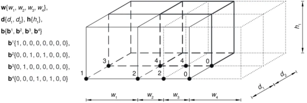
Design search space. A supercube (SC) is introduced to de-scribe a building spatial designBby means of a super-structure design search space representation. A supercube consisting of cells is described by four vectors:w,d,h,b. Equation 1 shows the variables used. Herebdescribes the existence of the cell with indicesi, jandkin space`, whereb`i,j,kwith a value ”1” means the celli,j,kis active and describes a part of space ` while ”0” means the cell is inactive. A space ` can thus be constructed out of the supercube cells that are activated for that space. Finally,wi,djandhkdescribe the continuous
w
1 w2
d1 d2
h1
1
3 4
2
w
3 w4
2 4
0 0
w{w
1,w2,w3,w4},
d{d
1,d2}, h{h1},
b{b1,b2,b3,b4}
b1{1, 0, 0, 0, 0, 0, 0, 0},
b2{0, 0, 1, 0, 1, 0, 0, 0},
b3{0, 1, 0, 0, 0, 0, 0, 0},
b4{0, 0, 0, 1, 0, 1, 0, 0}
Figure 1: Supercube representation of a building spatial design, space 2 and 4 are described by two cells each, the two right cells are not used to describe a room
i∈ {1, 2, ...,Nw} wi ∈R
j∈ {1, 2, ...,Nd} dj ∈R
k∈ {1, 2, ...,Nh} hk ∈R `∈ {1, 2, ...,Nspaces} b`i,j,k=
1, ifcelli,j,k∈space`
0, otherwise
(1)
Constraints and design modification. Building spatial design modification is performed by re-assigning cells to building spaces through changes of the binary variables and by modi-fying the dimensioning values of the supercube’s grid. Con-straints are introduced to the design search space so the search can focus on physically and technically feasible solutions. Con-straints can be checked by algorithms or, when stated as equa-tions, they can be part of the selection and generation of solu-tions. Stating constraints as equations has the advantage that their algebraic structure can be exploited by the employed op-timisation algorithms. The supercube representation is suitable for such algebraic expression of constraints, three constraints are presented here to demonstrate this suitability. The expres-sions enable the use of mathematical programming techniques like mixed integer non-linear programming (MINLP) which contribute to the efficiency of the optimisation. It should be noted that there may be differences between constraint repre-sentations and constraint implementations (not shown here). For example only ”1”-values in binary variables are stored in memory to avoid inefficient constraint checking by large zero spaces in vectorb.
Condition 1: Non Overlap Overlaps of building spaces are not allowed since they are not practical and might cause er-roneous results in subsequent design analysis. This needs to be checked because every space is represented by a separate bit-mask (enumerated by`) of all cells in the supercube, thus non-overlap is not automatically prevented in the representa-tion. Equation 2 achieves this by taking the sum of each cell over all masks. As a result of the binary representation, only if such a sum is smaller or equal to one, no overlap exists at that position.
∀i,j,k
Nspaces X
`=1
b`i,j,k≤1 (2)
Condition 2: Cuboid Spaces are constrained to cuboid shapes for practicality and to delimit the design space to a man-ageable size. To check this condition by means of an equation, first the supercube will be extended with a single layer of cells all around, and these new cells will be set to have no relation to any space (”0”), this extension is described by equation 3:
∀`:
∀i,j,k∈ {0, ...,Nw+1}
× {0, ...,Nd+1} × {0, ...,Nh+1}:
i=0∨ j=0∨k=0∨i=Nw+1∨j
=Nd+1∨k=Nh+1⇒b`i,j,k=0
(3)
Then for each building space`, in each direction pairs of ad-joining lines that run through the middles of the cells are imag-ined (e.g. for the z-direction a pair would be a line through all cells i1 = 2, j1 = 2 and a line through all cells i2 = 2, j2=3). Moving along a pair of lines,b`i,j,kvalues are processed as shown in equation 4 for thez-direction (as an example, of course all directions should be studied). To obtain a cuboid building space, if there is a change from zero to one in the bi-nary string it should occur at the same position (k-value) for both lines. Otherwise in the equation the sums as shown will hold different values and the difference will be non-zero. The same should hold for changes from one to zero, as seen in the second part of the equation. Note that equation 4 allows for the occurrence of multiple changes from one to zero and from zero to one. In other words a space could be cuboid, however could still have internal voids, e.g. a courtyard. Therefore condition 3 is introduced next.
∀`:
∀i1,j1,i2,j2: Nh X
k=1
k1−b`i
1,j1,k−1
b`i
1,j1,k − Nh X
k=1
k1−b`i
2,j2,k−1
b`i
2,j2,k Nh X
k=1 b`i
1,j1,k Nh X
k=1 b`i
2,j2,k = 0
∀i1,j1,i2,j2: Nh X
k=1
k1−b`i
1,j1,k+1
b`i
1,j1,k − Nh X
k=1
k1−b`i
2,j2,k+1
b`i
2,j2,k Nh X
k=1 b`i
1,j1,k Nh X
k=1 b`i
2,j2,k = 0 (4) ∀`:
∀i,j: XNh
k=0
1−b`i,j,kb`i,j,k+1≤1
∀i,k:
XNd
j=0
1−b`i,j,kb`i,j+1,k≤1
∀j,k: XNw
i=0
1−b`i,j,kb`i+1,j,k≤1
(5)
3.2. Super-structure free based representation
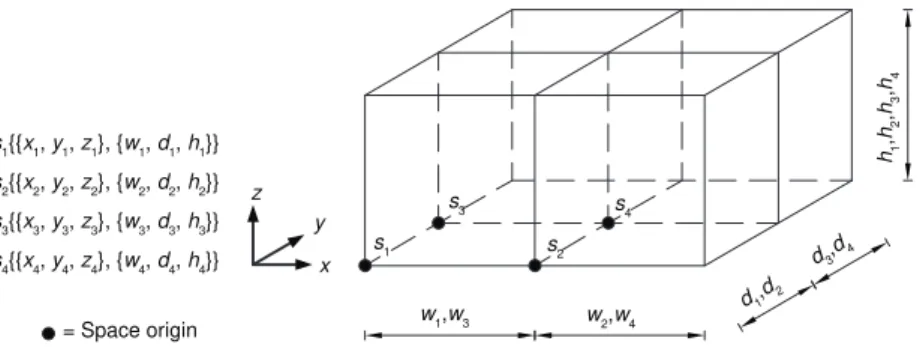
Design search space. A movable and sizeable (MS) represen-tation for spaces is introduced for the super-structure free de-sign space representation. For this, a building is described with a vectorsthat lists all the spaces. This vector is described by equation 6, in whichsirepresents a space,Cthe coordinates of
the space origin andDthe geometry of the space withw,dand
hthe width inx-, depth iny-, and height inz-direction, respec-tively. Figure 2 shows the building spatial design of figure 1 in the movable and sizeable representation.
s=ns1,s2, ...,sNspaceso where si=[C,D]
C=x,y,z
D=[w,d,h]
(6)
Constraints and design modification. The definition of spaces by location and dimensions allows an engineer to imagine the spatial properties of the space, the engineer can therefore in-tuitively define additional properties or modifications for that space. This intuitivity does however not count for the build-ing design itself, as relationships between spaces are defined implicitly. The movable sizable (MS) representation is thus most suitable for design modifications that operate on spaces rather than the entire building design, given that such opera-tions do not interfere with possible relaopera-tions between spaces. In the super-structure free approach, constraints are implicitly en-forced by using design modifications that naturally follow the constraints. Here, this is carried out via removal, scaling and di-vision of spaces. As an example, a modification of the building spatial design in figure 2 will be performed. Assume that after (e.g. structural or building physics performance) analyses, it is concluded that building spaceS3performs least well and thus
could better be removed as shown in equation 7. Accordingly, the remaining spaces are scaled (equation 8) to restore the ini-tial volume (V0) of the building design. To restore the number
of spaces, hereafter a (e.g. randomly selected) space is divided (equation 9) into two new spaces, resulting in a new spatial de-sign (equation 10). This process is further illustrated in figure 3 and has been used by [28] for real-world optimisation scenar-ios.
s{s1,s2,s3,s4} →s{s1,s2,s4} (7)
s→s· 3
r
V0
V (8)
s1{{x1,y1,z1},{w1,d1,h1}}
→
s5n{x1,y1,z1},n12w1,d1,h1oo s6nnx1+12w1,y1,z1o,n12w1,d1,h1oo
(9)
s{s2,s4,s5,s6} (10)
3.3. Discussion
w1,w3
d1,d2
h1
,
h2
,
h3
,
h4
s1
s3 s4
s2 z
x y
= Space origin w2,w4
d3,d4 s1{{x1, y1, z1}, {w1, d1, h1}}
s2{{x2, y2, z2}, {w2, d2, h2}} s3{{x3, y3, z3}, {w3, d3, h3}} s4{{x4, y4, z4}, {w4, d4, h4}}
Figure 2: Movable and sizeable representation of the building spatial design (first shown in figure 1)
s
3
½w
1 ½w1 w2,w4
d1
,
d2
d4
w
1, w3 w2, w4
d1
,
d2 d3
,
d4
w
5 w6 w2, w4
d2
,
d5
,
d6 d4
Space assessment Scale and subdivide New spatial design
50 125
110 115
s
4
s
1 s2 s5 s6
s
2
s
4
s
5 s6 s2
s
4
Building space to be deleted
Figure 3: Super-structure free modification, numbers in spaces in the left most figure represent performances of spaces (e.g. structural or building physics)
The super-structure free based approach to building optimi-sation can be developed even when only expertise of the built environment is available. Rules for modification of the consid-ered design are then based on knowledge and experience in the field. This approach can combine design variables in (math-ematically) unexpected ways and may therefore lead to new building designs that would otherwise not have been consid-ered. It also provides a fast way to navigate a large design search space, since it is not an exhaustive search of the en-tire design search space. The approach rather is a selection of other interesting parts of the design search space based on en-gineering knowledge and experience. However, this dynamic approach prevents the use of many classical search algorithms (global and parameter based search) and instead heuristic rules should be used to navigate the design space. Such heuristics are prone to find local optima and cannot provide high levels of confidence concerning these optima (although comparisons be-tween heuristics and global searches sometimes result in match-ing results). Compared to the super-structured approach, new design insights are more difficult to find when using heuristics, because fewer solutions are analysed and design evolution fol-lows a path that is defined by the heuristics.
To consider large design search spaces, it can be concluded that both approaches are eligible, although both have disadvan-tages as well: The super-structure approach is too costly in terms of computational effort and the super-structure free ap-proach cannot provide the optimum with a high level of
con-fidence. Therefore it is proposed to combine both approaches. Additionally, such a combination could enable the optimisation to discover both surprising designs and new design insights.
The presented representations are—in combination with the presented constraints—limited to only cuboid spaces. Re-leasing the cuboid spaces constraint will allow more complex spaces, which is desirable in real world design scenarios. This is possible with both representations, although the SC represen-tation would require a redefinition of some of the constraints and the MS representation requires a space to be defined as a collection of subspaces. This is however not implemented in the toolbox to avoid the additional complexity in the toolbox as it would distract from the focus of this research, namely to research and develop optimisation methodologies.
3.4. Combination of super-structured and super-structure free approaches
The combination of the approaches above is proposed by alternately employing each approach during the optimisation process for the same problem. This alternation requires mutual transformation between the two representations. To enable this, two algorithms have been developed which are presented in this subsection.
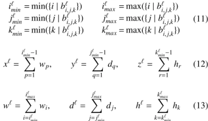
Supercube to movable and sizeable. To transform a building spatial design’s supercube representation into the movable and sizeable representation, it is suggested here to first find the smallest and largest indicesi,j,kfor the set of cells describing each space`as shown in equation 11. Space coordinatesx,y,z
can then be found as shown in equation 12, with the notion that if the smallest index equals 1, there is no term in the sum, and the degenerated sum is evaluated as 0 (which is appropriate here). The space dimensions are computed in a similar way us-ing the minimum and maximum indices as shown in equation 13.
i`min=min({i|b`i,j,k}) i`max =max({i|b`i,j,k}) j`min=min({j|b`i,j,k}) j`max=max({j|b`i,j,k}) kmin` =min({k|b`i,j,k}) k`max=max({k|b`i,j,k})
(11)
x` = i`min−1
X
p=1
wp, y`= j`min−1
X
q=1
dq, z` = k`min−1
X
r=1
hr (12)
w`= i`max
X
i=i`min
wi, d` = j`max
X
j=j`min
dj, h`= kmax`
X
k=k`min
hk (13)
Movable and sizeable to supercube. A transformation from movable and sizeable to supercube first requires three steps to compute the supercube dimensionsw,d,h. Step one—for each space—the minimum and maximum coordinate values should be found, i.e. for each space: {x,x+w}; {y,y+d};{z,z+h}. Step two, all these values are grouped into three lists (each for eitherx,yorzvalues), duplicate values are removed, and then each list is sorted in ascending order. Finally in the third step, vectorsw,d,hare computed from these lists. For example,w is computed aswi=xi+1−xifor everyi∈[1, ...,n−1] wheren
is the number of values stored in the sorted list.
Regarding vectorb, for each space`and for each celli,j, and
kthe (derived) cell’s coordinates are compared with the coor-dinates of the considered space. A cell is assigned to the con-sidered space if the cell coordinates are completely within the coordinates of the space, e.g. for the x-direction if: xspace ≤
xcell<xspace+wspace.
Validation. The above algorithms have been validated in [1] for overlaps in spaces, non-connected spaces, truncation er-rors, alterations in space identification, and fragmented spaces. Although errors due to truncations can occur and fragmented spaces may change a building spatial design, it was found that for the purposes of the toolbox the errors are insignificant and that fragmented spaces will not occur in the presented work.
4. Building analysis toolbox
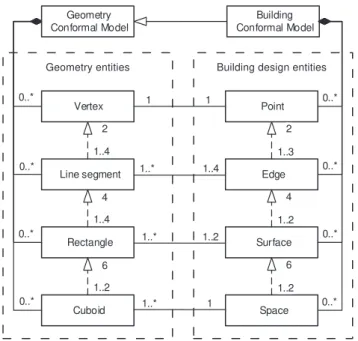
A toolbox to evaluate building spatial designs has been de-veloped in the form of a C++-library. This library forms an environment in which building spatial design optimisation can be developed and researched. The toolbox currently contains the following: structural design analysis, building physics anal-ysis, spatial design representations and a visualisation of these. Figure 4 shows the UML class diagram of the toolbox plus the modules that a user should still define, the toolbox’s visuali-sation is omitted for brevity. The diagram shows that a user should define an optimisation method but also the so-called de-sign grammars. These grammars generate domain specific in-formation that is required to evaluate the objective functions in that domain. A grammar will as such take a building spatial de-sign as input to generate domain specific information based on user defined design rules. The toolbox can be expanded to other disciplines as well by introducing new grammars, for exam-ple monetary or environmental costs could be included by im-plementing design rules to compute a model to calculate these costs for a building spatial design. This section first discusses the building spatial design representations, then structural- and building physics design analysis in the toolbox, and finally a benchmark is presented.
4.1. Spatial design
The spatial design environment consists of three main parts, namely the models for the MS-representation and the SC-representation but also a conformal model. Here a conformal model is the representation of a building design in which ge-ometry entities like line segments, rectangles or cuboids do not intersect with each other, but their vertices are allowed to coin-cide. For example when two walls are connected by a T-joint then the continuous wall is split into two rectangles at the inter-secting wall, see figure 5. This and similar splitting procedures are repeated in the conformation process until all intersections between spaces, surfaces, and line segments are represented in a model of smaller geometry entities. A conformal model is useful because domain relevant relationships vary over building edges, walls or spaces. For example, two walls with a T-joint connection will in a finite element model only be structurally connected if the nodes—at the joint—of both walls coincide. The conformation procedure enables a structural grammar to find such a joint so an appropriate design can be created ac-cordingly.
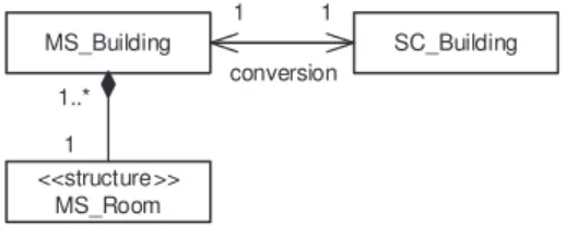
Building representations. Both the SC- and MS-representation have been implemented in separate classes, as illustrated in fig-ure 6. Conversion in either direction between the SC- and MS representations is implemented within those classes as well.
Structural Model Conformal Model Building Physics Model
Movable Sizeable Model
Design Grammar (s)
Optimisation Method
Super Cube Model
Realised by BP_Grammar Realised by
SD_Grammar
Figure 4: UML class diagram of the toolbox and the user defined program
T-joint of surfaces Varying dimensions of surfaces
Figure 5: Examples of non conformal surfaces that can be represented in a conformal model by geometry entities like vertices, lines, and rectangles
<<structure>> MS_Room
MS_Building SC_Building
1 1
conversion 1..*
1
Figure 6: UML class diagram of the movable sizeable (MS) and the supercube (SC) building representation classes
describe a building spatial design in a geometry model such that it is completely conformal. It is important to distinguish between the two because domain specific properties can depend on both geometric relations and building design relations. For example when a wind load is acting on a building wall that is described by multiple rectangles, then the rectangles are used to generate structural slabs, but the wall’s surface information is used to find the loads acting on these slabs. Geometry entities and building design entities are realised with lower dimensional entities and they are associated with the higher dimensional en-tities within their typology (i.e. design or geometry), e.g. a rectangle is realised with four line segments that on their turn are realised with two vertices each and also an association from that rectangle to one or more cuboids is made. Finally,
rela-tions between corresponding design and geometry entities are stored, e.g. a surface is associated to the rectangles that describe its conformal geometry and all surfaces that are described by a specific rectangle are associated to that rectangle. Adding and maintaining the mapping of figure 7 during the conformation of a design prevents a later iterative search for relevant relation-ships between geometry and building design entities.
0..*
0..* 0..*
0..* Geometry
Conformal Model
Vertex
Line segment
Rectangle
Cuboid
Point
Edge
Surface
Space Building Conformal Model
0..*
0..* 1
1
1..2 1..*
1 1..*
1..4 1..*
1..2 6 1..4 4 1..4 2
1..3 2
1..2 4
1..2 6 0..*
0..*
Geometry entities Building design entities
Figure 7: UML class diagram of the (orthogonal) conformation model
entities with all the relational mappings that are held by their parent (i.e. the entity that was split) and the parent’s associated entities, the parent is then tagged for deletion. It should be noted that a new geometry entity is only added to the geometry model if it is geometrically unique within the model, if it is not then the relational mapping of the matching entity is updated with the mapping of the new entity. Splitting of geometry entities invokes a recursion because new vertices can be created when an entity is split. These new vertices are first checked with all associated entities, which can be found by using the mapped relationships of the parent entity. When new intersections are found while splitting a geometry entity then these will first be split, thereby a recursion of splitting algorithms is invoked in the conformation process. Geometry entities that were tagged for deletion during the conformation process are deleted after all geometry entities have been checked for intersecting ver-tices.
4.2. Structural design
The structural design of a building is here an assembly of structural components, loads, and boundary conditions, e.g. columns; beams; slabs; wind loads; floor loads; and the con-straints that are imposed by a foundation. A structural design of a building needs to be evaluated on structural safety by as-sessing the strength, stiffness, and stability in the design. Such an evaluation can for example be carried out analytically or by means of the commonly used Finite Element Method (FEM). The toolbox employs FEM, in which the structural components of a design are modelled into smaller finite elements, nodal loads, and nodal constraints. The structural stiffness of each element is then derived for each node with respect to the posi-tions of all other nodes in the element. The stiffness terms of each element can then be assembled into a so-called global stiff -ness matrix K, and together with the nodal loads vectorfand
boundary conditions it is used to solve for the nodal displace-ments vectorugiven the equilibrium condition in equation 14.
f=Ku (14)
The optimisation objectives, i.e. the structural responses, can be calculated once vectors u and f and matrix K have been computed. Responses that are traditionally used for struc-tural design evaluation are strains, stresses, reaction forces or the displacements themselves and recently—for optimisation purposes—strain energies are used as well.
Element formulations. Three different element formulations have been implemented for structural design analysis in the toolbox: one for trusses, one for beams and one for flat shell elements. The element stiffness matrix of the truss elements is derived for an element with two nodes, each having three degrees of freedom (ux,uy,uz; withufor displacement) as is presented in [30]. The beam elements use an element stiffness matrix that has been derived for a two node element with each six degrees of freedom (ux,uy,uz,rx,ry,rz; withrfor rotation). The element formulation—as presented in [31]—accounts for axial forces, bending and torsional moments, and shear forces in two directions. Finally the formulation for a flat shell ele-ment is derived for a four node shell eleele-ment with six degrees of freedom per node (ux,uy,uz,rx,ry,rz). The formulation is a combination of a derivation for in-plane-behaviour as presented in [30] and out-of-plane behaviour [32] for which 2×2 numer-ical integration (Gaussian quadrature) is used to represent the displacement fields in the elements. Also a drilling stiffness is added to the stiffness matrix, its terms are equal to the mean of all terms in the element stiffness matrix in which the in- and out-of-plane behaviour are already determined. A flat shell el-ement using this formulation will offer resistance to in-plane normal forces, in- and out-of-plane shear forces, and torsional, drilling and bending moments.
find intersections: split geometry:
p5=p1+t·(p2−p1) if
(p2−p1)×(p4−p3) = 0 0<t<1
0<u<1
old lines:{{p1,p2},{p3,p4}}
with
t =(p3−p1)×(p4−p3) (p2−p1)×(p4−p3)
u =(p1−p3)×(p2−p1) (p4−p3)×(p2−p1)
new lines:{{p1,p5},{p2,p5},{p3,p5},{p4,p5}}
p4
p2
p1
p3
p4
p2
p1
p3 p5 p1 + t · (p2 - p1)
p3 + u · (p4 - p3)
Figure 8: Splitting of a line, first intersections are found then geometries are split. Rectangles and cuboids have similar procedures
Elements, nodes, nodal loads and nodal constraints can be added to the FE-model once a component has been meshed. Elements and nodes are initialised using the meshed points and the properties that are stored for a component. Constraints on a component are simply applied to all nodes that were meshed for that component. Finally loads are also applied to all meshed nodes, however their magnitude should be determined. This is carried out by splitting each element using the midpoints of line edges and quadrilaterals as shown in figure 9, the division temporarily creates new line segments or areas that are used to determine the magnitude of a load on a node in the element. Loads from different elements that share a common node are summed for that node.
Assembly and solving. A number of steps have to be com-pleted before the assembly of the FE-model into the form of equation 14 can start. Beginning with the initialisation of the nodes, where nodes are first checked for duplicity before they are added to the model. Elements are initialised thereafter, this process includes the following steps: associating nodes to the element; ordering of the associated nodes (the order of which is inherent to the derivation of the element formulation); updat-ing which degrees of freedom (DOF’s) are active in the FEM-model; and finally determining the value of the stiffness terms in the element stiffness matrix. After all the elements in a com-ponent have been initialised, then also the loads and constraints that act on it will be added to the nodes to which they have been meshed. Assembly of the FE-model can begin after all nodes, elements, loads and constraints have been initialised, and starts with indexing all DOF’s in the system by iterating over each element’s nodal freedom signature. Accordingly each term in each element stiffness matrix can be transformed into triplet form using the global DOF-indices, the complete global stiff -ness matrixKis as such defined in sparse form by a collection of triplets. Accordingly the load vector f is computed by ini-tialising a null vector to the size of the number of DOF’s, each load in each node is iterated and added to the load vector using the global indices of the nodal DOF’s. Constraints are handled as follows, global stiffness terms that depend on a constrained DOF are replaced with 1.0 if they are on the diagonal (to
pre-vent singular systems) and with 0.0 in any other case, terms in the load vector that act in a constrained DOF are replaced with 0.0.
The toolbox uses the Eigen C++template library [33] for all linear algebra in the finite element analysis, which provides vector templates, matrix templates, solvers and other linear al-gebra related algorithms. As such the stiffness matrix and the load vector have been assembled into instances of classes from the Eigen library and accordingly the system can be solved by using one of the solvers in the library.
Topology Optimisation. Another function that has been added to the structural design package is topology optimisation [16]. Topology optimisation aims to minimise an objective—e.g. strain energy—in an FE-model by varying element densities be-tween 0 and 100% while the total available material volume is constrained to a fraction of the total volume of elements. This method leads to structural topologies within an FE-model, fig-ure 10, which are then to be interpreted as a new structural design by either a designer or computer algorithm. Topology optimisation will be used in the toolbox to verify simulations of co-evolutionary design [28] in section 4.4. Also within the framework of this paper, it has been used to fine tune struc-tural designs that were generated by an iterative design gram-mar, which builds a structural design part by part based on con-current assessments of the structural performance [34].
4.3. Building physics
ℓ1 ℓ2 q in N/mm
1 2 3
p in N/mm2
A
1A
2n
= node
= midpoint = load
fn = (A1+A2).p
f2 = (ℓ1+ℓ2).q
Figure 9: Meshing of loads on nodes that have two line elements in common (left) or two quadrilateral elements in common (right)
Figure 10: Optimised topology of a solid structural design with live loads at floor heights and wind loading on the surfaces [35]
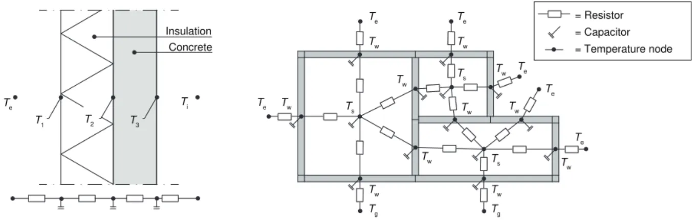
reasons, firstly only a low level of detail is required, this is pre-ferred because all information in the building physics model is generated by a design grammar thus more detail would also im-ply that a more sophisticated grammar is required. Secondly it is fast and thus it can be used to evaluate many designs in a rela-tively small amount of time, which is relevant for some optimi-sation methods. In [36] it is investigated how different simula-tion methods can work together by inversely modelling (i.e. fit-ting a model to data) the building thermal design to results from a more complex and detailed model or from real world data. It is concluded that the simple surogate model could still simu-late the same results when comparing it with the base model. An RC-network of a building can itself also have different lev-els of detail, for example phenomena like ventilation or solar irradiation add extra detail to the network. In [37] it is investi-gated how different levels of detail in an RC-network influence the simulation results. It was concluded that the most simpli-fied RC-network models still simulate results that are close to real world thermal behaviour of buildings. It should be noted that the aforementioned research uses inverse modelling to de-fine the parameters in the RC-networks, as such a direct mod-elling approach may not yield realistic values. However it can be concluded from the mentioned research that RC-networks do simulate realistic behaviour. These notions are important when real world problems are modelled, but for the building physics designs in the toolbox—that are derived from only a spatial design—a model is not expected to yield realistic
quan-titative values, but they are expected to yield realistic qualitative behaviour.
The terminology for RC-networks is borrowed from elec-trical engineering, where voltages and currents are simulated in a network of resistors and capacitors. Electrical components i.e. resistors and capacitors form a network in which each com-ponent describes a relationship that can be expressed in diff er-ential form. Thermal building properties can be mapped in a similar fashion, where a resistor is now modelled by the ther-mal conduction properties- and a capacitor by the heat capacity of the constructions and spaces in the building, see table 1. A system of first order ordinary differential equations (ODE’s) can be assembled from the relations that each of the components in the network describe. The system of ODE’s can then be used to simulate the dynamic problem that is described by the RC-network by solving the system over a specified simulation time, e.g. by an Eulerian method.
Table 1: RC-network components, the relations describing heat fluxΦq, and the units for temparatureT; heat resistanceR; heat capacitanceC; timet; and heat irradiationS
Component Relation Units
R
T1 T2 Φ
q= T2−RT1
T [K]
R[K/W]
C
T Φ
q=C·dTdt
C [J/K]
T [K]
t[s]
S T Φq=S S [W]
also a complete building, see figure 11.
System of temperature states. A building physics model in the toolbox is structured in a system of temperature state objects, see figure 12 for the UML class diagram. Here temperature states are specified into two child classes: one to resemble dependent and the other to resemble independent temperature states. Dependent temperature states (e.g. walls, floors and spaces) are simulated, whereas independent temperature states are input (such as weather data) and thus non dependent on the modelled system. Each dependent state is defined with a ca-pacitance, and each association between states is defined with a resistance. The system of state objects can then be translated into a system of ordinary first order differential equations as expressed in equation 15, wherexare the dependent states, u are the independent states, andAandBdescribe the system of resistors and capacitors. Additionally, for implementation pur-poses, two different dependent states—namely building con-structions and building spaces—are characterised in the tool-box.
˙
x=A·x+B·u (15)
Building constructions are here (parts of) walls and floors that consist out of one or more layers of material that each have a certain thickness and are represented by one temperature point in the RC-model. In the toolbox a construction is implemented as an aggregation of layers that each consist of a material. The resistance of a construction is not constant over its cross section. Therefore a location within the construction should be selected at which a lumped value for resistances and capacitances is to be determined, see figure 13. In the toolbox this point is by de-fault selected at half the thickness of the modelled construction. A construction’s resistance [K/W] from that point to its adja-cent temperature states is calculated according to equation 16, whereAis the wall’s surface in [m2], jdenotes each
contribut-ing layer,`thickness in [m], andλa heat conduction coefficient in [W/(K·m)]. The capacitance of a wallCw[J/K] is calculated as the sum of the capacitances of each materialkin the build-ing construction. This can be obtained followbuild-ing equation 17, whereCkis the specific heat capacity in [J/(kg·K)], andρthe density in [kg/m3] of each material. The location of the tem-perature state over the surface can be left undefined, under the assumption that the capacitances and resistances of a modelled construction are constant over its surface and that boundary ef-fects are not taken into account.
R=
X
j=1
`j
λj
/A (16)
C=
X
k=1
Ck·ρk·`k
·A (17)
Spaces are a special type of dependent temperature state in an RC-network model, because they are strongly influenced by
heating, cooling, occupation, and ventilation. Currently heat-ing, cooling and ventilation are accounted for in the simulation program, but thermal loads of e.g. people and equipment are not accounted for. This is to avoid an over-complication in the design grammar for a building physics design, since these loads would require design information such as room function, occu-pation, and time profiles. Currently only the number of Air Changes per Hour (ACH) and the total available heating and cooling power in spaces have been defined in a constant time profile.
The capacitance Cs of a space i is calculated with equa-tion 18, whereCair is the specific heat of air in [J/(K·kg)] (set to 1000 J/(K·kg)),ρair the density of air in [kg/m3] (set to 1.2
kg/m3) andV the volume of the space in [m3]. The factor 3 in the equation is an arbitrary number that takes into account any additional capacitance in the space, e.g. furniture. The resis-tance from a space to a construction is set to 0.14 K/W which is an empirical value for an air layer of approximately 10 mm.
Cs,i=V·ρair·Cair·3 (18)
Ventilation of a space is modelled as a loss of heat via a re-sistance to the weather profile, this is based on an air mass flow between the space and outside. The heat flux due to ventila-tionΦq,ventin [J/s] (i.e. Watt) in equation 19 is first expressed
based on the air mass flow and subsequently also equated to the heat loss as modelled by a resistanceRventin [K/W]. Solv-ing the equation for the resistance yields equation 20 in which the flow of mass ˙min [kg/s] can be substituted by equation 21 to yield equation 22. HereT is the temperature in [K],Rthe resistance that models the heat loss due to ventilation with air of another temperature state [K/W] and ACH is the ventilation rate in number of air changes per hour.
Φq,vent =m˙ ·Cair·(T2−T1)= T2−T1
Rvent
(19)
Rvent = 1
˙
m·Cair, (20)
˙
m=ρair·V· ACH
3600 (21)
Rvent =
Cair·ρair·V· ACH
3600 −1
(22)
Te
Insulation Concrete
T1 T2 T3
Ti Te T
s
Te Te
Te
Te
Tg Tg
Ts
Te Ts
Tw
Tw
Tw
Tw Tw
Tw
Tw
Tw
Tw Tw
Tw
= Resistor
= Capacitor = Temperature node
Figure 11: Two different levels of spatial detail for building thermal models using an RC-network model.
State
Dependent _State Indepent _State
Space
Weather_Profile
Wall Window
Floor
Ground_Profile
State_System 0..*
0..*
0..*
1 1 0..*
Adjacent to
0..*
Figure 12: UML class diagram of the building physics package
power is dependent on the temperature of a state. Equation 23 and figure 14 illustrate the function of such a P-switch for heat-ing, hereTsetis the temperature set point,Tvar is the length of
the temperature range over which the heating (Qheat) or
cool-ing power is variable (set to 10◦C), andQmaxis the maximum amount of power.
Qheat=
Qmax for T <Tset−Tvar Qmax· Tset−T
Tset−Tvar for Tset−Tvar≤T <Tset
0 for T ≥Tset
(23)
Independent state objects resemble external influences to the model, e.g. weather and soil. Information regarding these states should be provided in the form of a time profile of tem-peratures or irradiations by the user of the toolbox. Time pro-files can be arbitrary design values or real world measurements. Currently the toolbox can only use air temperature for simula-tions, data like solar irradiation is not considered.
Assembly and simulation. The assembly of the model starts by initialising temperature states for all spaces to the system. Ac-cordingly the temperature states of building constructions are initialised to the system, this process also handles the associa-tion with neighbouring states. On initialisaassocia-tion, dependent and independent temperature states are indexed with respect to their positions in state vectorsxandu. The state matricesAandB can be initialised once all temperature states have been added to the system. Once the RC-network is assembled into a sys-tem of ODE’s in the form of equation 15 it is solved for every consecutive time step in the simulation. After each time step the values of the independent temperature states are updated. A C++library that offers generic implementations of algorithms for numerical solving of ordinary differential equations is em-ployed to solve the system, which is the odeint library [38] that is part of an overarching library: Boost [39].
4.4. Toolbox benchmark
Building spatial design optimisation has been carried out in [28] by means of simulations of co-evolutionary design pro-cesses to minimise the strain energy in the structural design. The toolbox presented here has successfully been benchmarked with one of the simulations that were performed in that paper, see figure 15. The used structural design grammar creates—for each space—four flat shell components for the walls of a space and one flat shell component at the top of a space. Each flat shell component in the structural design is assigned a thickness of 150 mm and material properties that resemble concrete, i.e. a Young’s modulus of 30000 N/mm2and a Poission’s ratio of 0.3.
A live load case of 1.8 kN/m2in negativez-direction is applied to each horizontally aligned flat shell component. Additionally four wind load cases (in+x,+y,−x,−ydirections) are applied to each vertically aligned flat shell that does not have a space at both sides of the flat shell. Each wind load case consists of three different types, i.e. pressure (1.0 kN/m2), suction (0.8 kN/m2) and shear (0.4 kN/m2), which are applied to a flat shell
ℓ1
½(ℓ1+ℓ2) ½(ℓ1+ℓ2)
ℓ2
Insulation:
λins in [W/(K∙m)]
Cins in [J/(K∙m)]
ρins in [kg/m³]
Transitional air layer:
Rair,s,1 in [m2∙K/(W)]
Concrete:
λcon in [W/(K∙m)]
Ccon in [J/(K∙m)]
ρcon in [kg/m³]
Transitional air layer:
Rair,s,2 in [m2∙K/(W)]
Ts,1 Tw,1 Ts,2
Cw,1
R1 R2
R1= `1 λins
+`2−`1 2·λcon
+Rair,s,1 !
/A [K/(W)]
R2= `1+`2 2·λcon
+Rair,s,2 !
/A [K/(W)]
Cw,1=`1·A·Cins·ρins
+`2·A·Ccon·ρcon [J/(K)]
−Ais the wall’s surface area [m2]
−ρis a materials density [kg/m3]
−λis a materials heat
conduction coefficient [W/(K·m)]
Figure 13: Calculation example of lumped resistance and capacitance of a construction
Tset−Tvar Tset
Temperature [K] Qmax
Heating
po
w
er
[
W
]
Figure 14: P-switch that controls heating in spaces, a similar function is used for cooling
completing the structural design grammar. The optimisation procedure is carried out by first performing topology optimisa-tion on the structural design, which results in an optimal density for each structural finite element. Element densities are clus-tered into eight clusters using thek-means algorithm and sub-sequently the elements in the four lowest clusters are deleted. The number of deleted elements is then used as a measure for the performance of each space and each space is then sorted with respect to the number of deleted elements. Accordingly half of the spaces with the highest number of deleted elements is removed from the building spatial design and additionally any remaining spaces that have an equal amount of deleted el-ements as one of the removed spaces are also removed. Finally all remaining spaces are split and subsequently scaled inx- and
y-dimensions by a factor of √2 to bring the design back to its original number of spaces and volume, although it should be noted that spaces and thus volume may be lost in the previous step. This procedure is performed iteratively until a stopping criterion has been reached, which is here set to the third itera-tion.
It should be noted that some differences between text and code were found in [28]. Firstly in the distribution of live load-ing it is described that loads are a half at the edges and a quarter at the corners of flat shell components, however this is only the case when these loads are located somewhere on the sur-face of the bounding box of the complete building spatial de-sign. Secondly, clustering of element densities is not performed
after clusters are initiated. Also, for topology optimisation it should be noted that element volume sensitivities with respect to changes in element density are not considered in the compu-tation of the gradient and that the volume constraint is imple-mented as a constraint that keeps the average density over all elements constant. Finally the magnitude of the live loading is given as 1.8 kN/m2, while it is actually simulated as 7.2 kN/m2. These differences were temporarily implemented in the toolbox presented here to successfully benchmark it to that used in [28]. To evaluate program efficiency both the code as used in [28] and the toolbox that is presented in this paper have been used to simulate the problem of figure 15 on an HP Z440 worksta-tion (Intel Xeon E5-1650 v3 @3.5 GHz, 16 GB RAM @1600 MHz), simulation times were around 22 hour for the code used in [28] and 33 minutes for the toolbox presented here.
5. Toolbox demonstration
This section presents some early work in the development of simulations of co-evolutionary design processes, of which those presented here are algorithms that remove and add spaces based on space performances, see figure 16. The presented work shows the promise of simulations of co-evolutionary de-sign processes over a super-structured approach, but it also shows the challenges that should still be overcome. Only super-structure free optimisation is demonstrated here, application of the toolbox in super-structured optimisation can be found in [40, 41, 42, 43], in which the supercube representation is used with a multi-disciplinary evolutionary optimisation algo-rithm to optimise for structural performance and building sur-face area.
943 .5 Nm Total Strain energy
373 .6 Nm
499 .0 Nm Optimal structural design
Building spatial design
Reference case Toolbox
Figure 15: Successful benchmark of the toolbox with a reference case that is presented in [28]
indexed by spaceiand discipline j. Fis normalised into ma-trixPusing equation 24, whereminjandmaxjare respectively
the minimum and maximum terms in the jth column. For each spaceiand each disciplinejthe normalised space performances are stored. For single disciplinary modification all spaces are sorted in a list in ascending order of normalised space perfor-mance. Multi-disciplinary modification would require to first evaluate the normalised space performances of each discipline per space and express this evaluation into one normalised space performance before such a list can be computed. The top half of the spaces in the ordered list of spaces is then removed from the design, and to ensure a symmetric design also any remain-ing spaces that have the same normalised space performance as the last removed space are removed. Accordingly all spaces are split in half along their longest horizontal dimensions, or if both are equally long then they are split in half along thex -direction. Note that if more than half of the spaces are removed, then this method leads to a loss of spaces, which is allowed for the demonstration. Finally the horizontal dimensions in the de-sign are scaled with a factor of
√
2 to bring the design back to its original volume (assuming that no spaces were lost). One cy-cle of the simulation of co-evolutionary design processes is then completed, a stopping criterion terminates the process, which is in this demonstration met after two cycles have been completed.
Pi,j= Fi,j−minj maxj−minj
(24)
It should be noted that the process described above is not an explicitly directed search for better performances. As such it can also not be defined as a global or local search. Also no hard constraints to guarantee valid designs are defined. However knowledge and experience can be used to define design mod-ifications such that better and valid designs can be found, e.g. [28] shows how well this can work. Moreover, using different design modifications together can improve the chance to find better performing designs. Although this is an interesting topic, it is not elaborated here for brevity and it is not the purpose of the demonstration to address this topic. Moreover it should be noted that the demonstration entails only single disciplines. A multi-disciplinary search would introduce multiple new chal-lenges to this paper, multiple disciplines have—for clarity and brevity—not been considered in the demonstration.
5.1. Structural building design
Initial building
spatial design Movable Sizablemodel Conformation Conformal model
Domain specific models Domain specific analysis
Design performances
Pi,j Design modification
Domain specific design grammars
Stop cycle ?
Final building spatial design yes
no New building spatial design
Figure 16: Process diagram of the simulation of co-evolutionary design processes that is used for the toolbox demonstration
contradiction is common for compliance based optimisation, it is also found in e.g. topology optimisation. For this simulation a design grammar is defined by assigning a flat shell component with a thickness of 150 mm, Youngs modulus of 30000 N/mm2
and a Poisson’s ratio of 0.3 to all rectangles in the conformal building spatial design that belong to a surface. A live load case is defined with loads of 5.0 kN/m2in−zdirection that are
added to each horizontal flat shell component and wind loads are assigned to each surface in the conformal design that is not related to more than one space. Four load cases are defined for these wind loads, +x,+y,−xand −y, a wind load itself is di-vided into three components, pressure 1.0 kN/m2, suction 0.8 kN/m2and shear 0.4 kN/m2, which are each added to a surface depending on its orientation and the wind direction. Finally the design grammar applies line constraints to each edge at the bot-tom of the building spatial design, the structural design is then meshed using 10 divisions in each dimension and it is solved using an LDLT solver [33].
Figure 17 shows the results after two cycles. After the first cycle there is a clear improvement of the strain energy in the structural design, however after the second cycle the strain en-ergy is even higher than that of the initial design. The results are somewhat similar as the benchmark in figure 15, where a similar effect is observed. This shows that this approach is not a directed search, however it also shows that significant im-provements could be found after just one iteration. These quick improvement steps suggest that a super-structure free approach may influence optimisation times significantly when this insight is used to limit a super-structured design search space to for ex-ample a maximum of two stories. From a structural point of view the results may be explained by the fact that flat buildings are more optimal since tall buildings lead to an accumulation of structural loads, whereas flat buildings transfer loads towards the foundation in a shorter path.
5.2. Thermal building design
The objective is to minimise the heating and cooling energy that is required to maintain the building between set tempera-tures. This is measured by simulating the heating and cooling
energy demand in each space, the total energy demand is then computed as the sum of heating and cooling energies over the simulation time and over each space. To realise a thermal simu-lation, the building physics grammar assigns one building con-struction to each of the rectangles that belong to a surface in the building spatial design that consists of a 150 mm thick layer of concrete with a specific weight of 2400 kg/m3, a specific heat
capacity of 850 J/(K·kg) and a thermal conduction coefficient of 1.8 W/(K·m). Rectangles that belong to only one surface (i.e. one adjacent space or external wall) are assigned an additional layer to their construction, namely a layer of insulation of 150 mm thick with a specific weight of 60 kg/m3, a specific heat capacity of 850 J/(K·kg) and a thermal conduction coefficient of 0.04 W/(K·m). The temperature set point for heating is set at 20◦C and the set point for cooling at 25◦C, the total available heating and cooling power in spaces is set to 100 W/m3. The
180 .6 Nm
108 .8 Nm
205 .8 Nm
Building spatial design Analysis of the
structural design
Space performance Total strain
energy
0.0 ≤ Pi,j < 0.2 0.2 ≤ Pi,j < 0.4
Space performance legend: (the legend for the structural design analysis is not given nor relevant)
0.4 ≤ Pi,j < 0.6 0.6 ≤ Pi,j < 0.8 0.8 ≤ Pi,j ≤ 1.0
Figure 17: Simulation of building structural design process, normalised space performances are determined according equation 24. The last iteration performs worst, which can here be explained due to more surfaces being exposed to wind and floor loads compared to preceding iterations.
Figure 18 shows the results after two iterations. From these results it can be observed that the used design modification can-not find a better solution in the first two iterations, which sug-gests that a different design modification should be used. From a thermal point of view the spaces at a corner of a building spa-tial design will be suboptimal since these have the most surface through which heat is lost and looking at the results it can be observed that those spaces are in fact removed. However in the worst case when a corner space is removed this will introduce three new corner spaces, as such it can indeed be concluded that a different design modification should be used to find a ther-mally optimal building spatial design. A more suitable design modification would not only take into account the performance of spaces, but could for example also take into account their relative location in the building.
6. Conclusions and outlook
This paper has elaborated on different optimisation ap-proaches for building spatial design and has presented a toolbox to effectuate these approaches for further research. Conclusions and outlooks that have been presented in this paper are summa-rized below.
The difference between structured versus super-structure free approaches is a recurrent theme in specific fields of optimisation [2]. In this paper, for the super-structured ap-proach, a supercube representation has been proposed, in which
a fixed number of cells can be switched on and off to gener-ate different building spatial designs, while constraints ensure practical designs, e.g. no overlap of spaces should occur. A super-structure free approach has been developed by a movable and sizeable representation, listing the building spaces with their position and dimensions, and allowing these spaces to be deleted, split, and resized, as such automatically following the constraints.
Algorithms have been derived to transform the supercube representation into the movable and sizeable representation and vice versa. These algorithms have been verified in [1] for successful operation when overlaps in spaces, non-connected spaces, truncation errors, alterations in space identification, and fragmented spaces occur.
A toolbox has been developed in which the presented spa-tial design representations can be evaluated for their structural and thermal behaviour. The toolbox enables users to develop and write their own optimisation procedures and design gram-mars. Also a benchmark has been presented in which the tool-box has successfully simulated a problem that is presented in other work.
63 .8 MWh
71 .0 MWh
66 .9 MWh Heating and cooling
energy Space performance
Building physics design Building spatial design
0.0 ≤ Pi,j < 0.2 0.2 ≤ Pi,j < 0.4 0.4 ≤ Pi,j < 0.6 0.6 ≤ Pi,j < 0.8 0.8 ≤ Pi,j ≤ 1.0
Space performance legend:
Figure 18: Simulation of building thermal design process, normalised space performances are determined according equation 24
toolbox and also to show the promises and the challenges of this method.
In the near future, a multi-disciplinary design modification will be developed based on simulations of co-evolutionary de-sign processes. Subsequently an optimisation approach will be developed where both representations are used alternately: The super-structured approach will allow a dedicated optimisation algorithm to find a global optimum [40, 42], whereas this so-lution in a super-structure free approach can be used by the developed design modification to explore more freely another (possibly local) optimum. As such the design space is cycli-cally both explored in-depth (via the super-structure) and glob-ally (via the super-structure free representation). This method is demonstrated in [43].
Acknowledgements
This work is part of the TTW-Open Technology Programme with project number 13596, which is (partly) financed by the Netherlands Organisation for Scientific Research (NWO). The work of J.M. Davila Delgado is acknowledged here for his con-tributions in the research on simulations of co-evolutionary de-sign processes for building spatial dede-signs. The authors would also like to thank R.C.G.M. Loonen for his assistance with and his knowledge of building thermal simulations.
References
[1] S. Boonstra, K. van der Blom, H. Hofmeyer, R. Amor, M. T. M. Em-merich, Super-structure and super-structure free design search space rep-resentations for a building spatial design in multi-disciplinary building optimisation, in: ICE 2016, Electronic proceedings of the 23rd EG-ICE workshop, Jagiellonian University ZPGK, 2016, pp. 281–290. [2] P. Voll, M. Lampe, G. Wrobel, A. Bardow, Superstructure-free synthesis
and optimization of distributed industrial energy supply systems, Energy 45 (1) (2012) 424–435. doi:10.1016/j.energy.2012.01.041.
[3] M. Wetter, Simulation-based building energy optimization, Ph.D. thesis, University of California, Berkeley (2004).
[4] D. Tuhus-Dubrow, M. Krarti, Genetic-algorithm based approach to opti-mize building envelope design for residential buildings, Building and En-vironment 45 (7) (2010) 1574–1581. doi:10.1016/j.buildenv.2010.01.005. [5] Q. Q. Liang, Y. M. Xie, G. P. Steven, Optimal Topology Design of Bracing Systems for Multistory Steel Frames, Journal of Struc-tural Engineering 126 (7) (2000) 823–829. doi:10.1061/ (ASCE)0733-9445(2000)126:7(823).
[6] R. Baldock, K. Shea, Structural Topology Optimization of Braced Steel Frameworks Using Genetic Programming, in: Intelligent Computing in Engineering and Architecture: 13th EG-ICE Workshop 2006, Ascona, Switzerland, June 25-30, 2006, Revised Selected Papers, Springer-Verlag Berlin Heidelberg, 2006, pp. 54–61. doi:10.1007/11888598 6.
[7] B. Steiner, E. Mousavian, F. M. Saradj, M. Wimmer, P. Musialski, Integrated structural–architectural design for interactive planning, in: Computer Graphics Forum, Wiley Online Library, 2016, pp. 80–94. doi:10.1111/cgf.12996.
[8] W. Wang, R. Zmeureanu, H. Rivard, Applying multi-objective genetic algorithms in green building design optimization, Building and Environ-ment 40 (11) (2005) 1512–1525. doi:10.1016/j.buildenv.2004.11.017. [9] J. A. Wright, H. A. Loosemore, R. Farmani, Optimization of


![Figure 15: Successful benchmark of the toolbox with a reference case that is presented in [28]](https://thumb-us.123doks.com/thumbv2/123dok_us/8313979.2202391/14.892.133.768.123.575/figure-successful-benchmark-toolbox-reference-case-presented.webp)
