An Immersed Boundary Method with Divergence-Free Velocity
Interpolation and Force Spreading
Yuanxun Bao∗, Aleksandar Donev, David M. McQueen, Charles S. Peskin
Courant Institute of Mathematical Sciences, New York University, 251 Mercer Street, New York, NY, USA
Boyce E. Griffith
Departments of Mathematics and Biomedical Engineering, Carolina Center for Interdisciplinary Applied Mathematics, and McAllister Heart Institute, University of North Carolina, Chapel Hill, NC, USA
Abstract
The Immersed Boundary (IB) method is a mathematical framework for constructing ro-bust numerical methods to study fluid-structure interaction in problems involving an elastic structure immersed in a viscous fluid. The IB formulation uses an Eulerian representation of the fluid and a Lagrangian representation of the structure. The Lagrangian and Eulerian frames are coupled by integral transforms with delta function kernels. The discretized IB equations use approximations to these transforms with regularized delta function kernels to interpolate the fluid velocity to the structure, and to spread structural forces to the fluid. It is well-known that the conventional IB method can suffer from poor volume conservation since the interpolated Lagrangian velocity field is not generally divergence-free, and so this can cause spurious volume changes. In practice, the lack of volume conservation is espe-cially pronounced for cases where there are large pressure differences across thin structural boundaries. The aim of this paper is to greatly reduce the volume error of the IB method by introducing velocity-interpolation and force-spreading schemes with the properties that the interpolated velocity field in which the structure moves is at least C1 and satisfies a continuous divergence-free condition, and that the force-spreading operator is the adjoint of the velocity-interpolation operator. We confirm through numerical experiments in two and
∗Corresponding author
Email addresses: [email protected](Yuanxun Bao),[email protected](Aleksandar Donev),[email protected](David M. McQueen),[email protected](Charles S. Peskin),
[email protected](Boyce E. Griffith)
three spatial dimensions that this new IB method is able to achieve substantial improvement in volume conservation compared to other existing IB methods, at the expense of a modest increase in the computational cost. Further, the new method provides smoother Lagrangian forces (tractions) than traditional IB methods. The method presented here is restricted to periodic computational domains. Its generalization to non-periodic domains is important future work.
Keywords: Immersed boundary method, fluid-structure interaction, incompressible flow, volume conservation, velocity interpolation, force spreading
1. Introduction
The Immersed Boundary (IB) method [34] is a general mathematical framework for the numerical solution of fluid-structure interaction problems arising in biological and engineer-ing applications. The IB method was introduced to simulate flow patterns around the heart valves [32, 33], and since its success in modeling cardiac fluid dynamics [31, 15, 16, 14], it has been extended and applied to various other applications, including but not limited to motion of biological swimmers [3, 30], dynamics of red-blood cells [9] and dry foam [21, 22], and rigid body motion [20, 43].
The essence of the IB method as a numerical scheme lies in its simple way of coupling an Eulerian representation of the fluid and a Lagrangian representation of the structure. The
even higher order for problems with singular forcing at the sharp interface. Notable examples include, the Immersed Interface Method (IIM) [28, 27], and more recently, a new method known as Immersed Boundary Smooth Extension [37, 38]. Our focus here, however, is on improving the volume conservation properties of the IB method.
As an immediate consequence of fluid incompressibility, which is one of the basic as-sumptions of the IB formulation, the volume enclosed by the immersed structure is exactly conserved as it deforms and moves with the fluid in the continuum setting. Thus, a desirable feature of an IB method is to conserve volume as nearly as possible. In practice, however, it is observed that, even in the simplest case of a quasi-static pressurized membrane [17], the conventional IB method (regardless of collocated- or staggered-grid discretization) produces volume error that persistently grows in time, as if fluid “leaks” through the boundary. An in-tuitive explanation for this “leak” is that fluid is “squeezing” between the marker points used to discretize the boundary in a conventional IB method; however, this is not the full story, because refining the Lagrangian discretization does not improve the volume conservation of the method for a fixed Eulerian discretization.
In the conventional IB method, we can extend the notion of velocity interpolation to any point in the domain (not restricted to the immersed structure), denoted here with an italic
X. The continuous interpolated velocity field can be written as U(X) = (Ju)(X), where
J denotes the continuous interpolation operator that interpolates the velocity at X from the discrete fluid velocity u. If a closed surface moves with velocity that is continuously
zero as the discretization of the surface is refined. Peskin and Printz realized that the major cause of poor volume conservation of IBCollocated is that thecontinuousinterpolated velocity field given by the conventional IB interpolation operator (denoted by JIB) is not
continuously divergence-free [35], despite that the discrete fluid velocity is enforced to be
further improvement in volume conservation by ensuring that the interpolated velocity is constructed to be nearly or exactly divergence-free. We note that the methods designed to improve the convergence rate of IB methods, such as IIM [28, 27] and the Blob-Projection method [5], also improve volume conservation, because the solution near the interface is computed more accurately. These methods, however, are somewhat more complex and less generalizable than the conventional IB method.
This paper is concerned with further improving volume conservation of IBMAC by con-structing a continuous velocity-interpolation operator J that is divergence-free in the con-tinuous sense. The discrete IB interpolation operator S? is simply the restriction of J to the Lagrangian markers. The key idea introduced in this paper is first to construct adiscrete vector potential that lives on anedge-centered staggered grid from the discretely divergence-free fluid velocity, and then to apply the conventional IB interpolation scheme to obtain a
continuum vector potential, from which the interpolated velocity field is obtained by apply-ing the continuum curl operator. Note that the existence of the discrete vector potential relies on the fact that the discrete velocity field is discretely divergence-free. The interpolated velocity field obtained in this manner is guaranteed to be continuously divergence-free, since the divergence of the curl of any vector field is zero. We also propose a new force-spreading operator S that is defined to be the new adjoint of the interpolation operator S?, so that Lagrangian-Eulerian interaction conserves energy. The Eulerian force density that is the result of applying this force-spreading operator to a Lagrangian force field turns out to be discretely divergence-free, so we refer to this new force-spreading operation as divergence-free force spreading. We name the IB method equipped with the new interpolation and spreading operators as the Divergence-Free Immersed Boundary (DFIB) method. As presented here, the DFIB method is limited to periodic domains.
delta function ∇δh instead of only δh. We confirm through various numerical tests in both two and three spatial dimensions that the DFIB method is able to reduce volume error by several orders of magnitude compared to IBMAC and IBModified at the expense of only a modest increase in the computational cost. Moreover, we confirm that the volume error for DFIB decreases as the Lagrangian mesh is refined with the Eulerian grid size held fixed, which is not the case in the conventional IB method [35]. In addition to the substantial improvement in volume conservation, the DFIB method is quite straightforward to realize from an existing modular IB code with staggered-grid discretization, that is, by simply switching to the new velocity-interpolation and force-spreading schemes while leaving the fluid solver and time-stepping scheme unchanged.
The rest of the paper is organized as follows. In Sec. 2, we begin by giving a brief description of the continuum equations of motion in the IB framework. Then we define the staggered grid on which the fluid variables live and introduce the spatial discretization of the equations of motion. Sec. 3 introduces the two main contributions of this paper: divergence-free velocity interpolation and force spreading. In Sec. 4, we present a formally second-order time-stepping scheme that is used to evolve the spatially-discretized equations, followed by a cost comparison of DFIB and IBMAC. Numerical examples of applying DFIB to problems in two and three spatial dimensions are presented in Sec. 5, where the volume-conserving characteristics of the new scheme are assessed.
2. Equations of motion and spatial discretization
2.1. Equations of motion
This section provides a brief description of the continuum equations of motion in the IB framework [34]. We assume a neutrally-buoyant elastic structure Γ that is described by the Lagrangian variabless, immersed in a viscous incompressible fluid occupying the whole fluid domain Ω ⊂R3 that is described by the Eulerian variables x. Eqs. (2.1) and (2.2) are the
fluid-structure coupled equations are:
ρ
∂u
∂t +u· ∇u
+∇p=µ∇2u+f, (2.1)
∇ ·u= 0, (2.2)
f(x, t) =
Z
Γ
F(s, t)δ(x−X(s, t)) ds, (2.3)
∂X
∂t (s, t) =u(X(s, t), t) =
Z
Ω
u(x, t)δ(x−X(s, t)) dx, (2.4)
F(s, t) =F[X(·, t) ;s] =−δE
δX(s, t). (2.5)
Eqs. (2.3) and (2.4) are the fluid-structure interaction equations that couple the Eulerian and the Lagrangian variables. Eq. (2.3) relates the Lagrangian force density F(s, t) to the Eulerian force density f(x, t) using the Dirac delta function, where X(s, t) is the physical position of the Lagrangian point s. Eq. (2.4) is simply the no-slip boundary condition of the Lagrangian structure, i.e., the Lagrangian point X(s, t) moves at the same velocity as the fluid at that point. In Eq. (2.5), the system is closed by expressing the Lagrangian force density F(s, t) in the form of a force density functional F[X(·, t) ;s], which in many cases can be derived from an elastic energy functionalE[X(·, t) ;s] by taking the variational derivative, denoted here by δ/δX, of the elastic energy.
2.2. Spatial discretization
Throughout the paper, we assume the fluid occupies a periodic domain Ω = [0, L]3 that
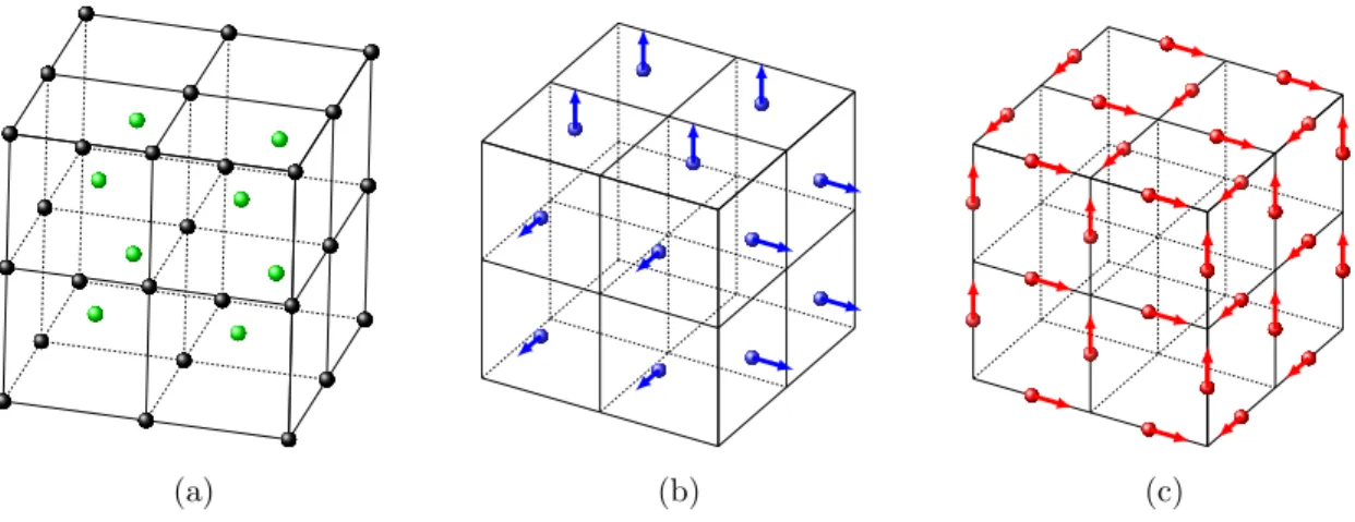
is discretized by a uniform N ×N ×N Cartesian grid with meshwidth h = NL. Each grid cell is indexed by (i, j, k) for i, j, k = 0, . . . , N −1. For the Eulerian fluid equations, we use the staggered-grid discretization, in which the pressure p is defined on the cell-centered grid (Fig. 1a), denoted by C, i.e., at positions xi,j,k = ((i+ 12)h,(j + 12)h,(k + 12)h). The discrete fluid velocityuis defined on the face-centered grid (Fig. 1b), denoted byF, with each component perpendicular to the corresponding cell faces,i.e., at positionsxi−1
2, j, k,xi, j− 1 2, k
and xi, j, k−1
2 for each velocity component respectively. We also introduce two additional
shifted grids: the node-centered grid (Fig. 1a) for scalar grid functions, denoted by N , i.e., at positions xi−1
2, j− 1 2, k−
1
2, and the edge-centered grid (Fig. 1c) for vector grid functions,
(a) (b) (c)
Fig. 1: Staggered grids on which discrete grid functions are defined. (a) Cell-centered (green) and
node-centered (black) grids for scalar functions. (b) Face-node-centered grid for vector grid functions. (c) Edge-node-centered
grid for vector grid functions.
i.e., at positions xi, j−1 2, k−
1 2, xi−
1 2, j, k−
1
2 and xi− 1 2, j−
1
2, k for each component respectively. In
Sec. 3, we will use these half-shifted staggered grids to construct divergence-free velocity interpolation and force spreading.
To discretize the differential operators in Eqs. (2.1) and (2.2), we introduce the central difference operators corresponding to the partial derivatives ∂/∂xα,
Dhαϕ:= ϕ(x+ h
2eα)−ϕ(x− h 2eα)
h , α= 1,2,3, (2.6)
whereϕis a scalar grid function and{e1,e2,e3}is the standard basis of R3. We can use Dαh to define the discrete gradient, divergence and curl operators:
Ghϕ:= (D1hϕ, Dh2ϕ, D3hϕ), (2.7)
Dh·v:=Dαhvα, (2.8)
Dh×v:=ijkDjhvk, (2.9)
where v is a vector grid function, ijk is the totally antisymmetric tensor, and the Einstein summation convention is used here. The discrete differential operators may be defined on different pairs of domain and range (half-shifted staggered grids), and therefore, in a slight abuse of notation, we will use the same notation to denote the different operators,
Dh·:v(E)−→ϕ(N) or v(F)−→ϕ(C), (2.11)
Dh×:v(E)−→v(F) or v(F)−→v(E). (2.12)
Although the curl operator does not appear in the equations of motion explicitly, we define it here for use in Sec. 3. The discrete scalar Laplacian operator can be defined byLh =Dh·Gh, which yields the familiar compact second-order approximation to ∇2:
Lhϕ:=
3
X
α=1
ϕ(x+heα)−2ϕ(x) +ϕ(x−heα)
h2 . (2.13)
Note that the range and domain of Lh are a set of grid functions defined on the same grid, and that grid can be C or N or any of the three subgrids of E or F on which the different components of vector-valued functions are defined. We will use the notation Lh to denote the discrete vector Laplacian operator that applies (the appropriately shifted) Lh to each component of a vector grid function.
2.2.1. Advection
We follow the same treatment of discretization of the advection term as in earlier pre-sentations of the IB method [7]. From the incompressibility of the fluid flow ∇ ·u = 0, we can write the advection term in the skew-symmetric form
[(u· ∇)u]α = 1
2u·(∇uα) + 1
2∇ ·(uuα), α= 1,2,3. (2.14) LetN(u) denote the discretization of Eq. (2.14), and we define
[N(u)]α = 1 2u˜·G
2hu α+
1 2D
2h·(˜uu
α), α= 1,2,3, (2.15) where ˜u denotes an averaged collocated advective velocity whose components all live on the same grid as uα. The advective velocity ˜uin [7] is obtained by using the same interpolation scheme as the one used for moving the immersed structure. In our work, we simply take the average of u on the grid. For example, the three components of ˜u in the x-component equation are
˜
u1 =u1(xi−1 2,j,k),
˜
u2 =
u2(xi,j−1
2,k) +u2(xi,j+ 1
2,k) +u2(xi−1,j− 1
2,k) +u2(xi−1,j+ 1 2,k)
˜
u3 =
u3(xi,j,k−1
2) +u3(xi,j,k+ 1
2) +u3(xi−1,j,k− 1
2) +u3(xi−1,j,k+ 1 2)
4 .
Note that in they- and z-component equations, we need different averages ofu to construct ˜
u. We choose to use the wide-stencil operators in Eq. (2.15) so that the resulting grid functions are all defined on the same grid as uα. A more compact discretization of the advection term has been previously described in [17, 13, 42].
2.2.2. Fluid-Structure Interaction
The immersed structure Γ is discretized by a Lagrangian mesh of M points or markers, denoted here by a non-italic X = {Xm}
M
m=1, and the discrete Lagrangian force densities
defined on the Lagrangian markers are F = {Fm}Mm=1. As discussed in the introduction, we can extend the notion of velocity interpolation to any point X in the domain, not just restricted to the Lagrangian markers X, and define a continuous interpolated velocity field
U(X) = (Ju)(X). In the conventional IB method, the continuous velocity-interpolation operator JIB can be defined as
U(X) = (JIBu)(X) :=
X
x∈F
u(x)δh(x−X)h3. (2.16)
We note that the interpolated velocity field given by Eq. (2.16) is notgenerally divergence-free with respect to the continuum divergence operator1, i.e., generally
(∇ ·U)(X) = −X
x∈F
u(x)·(∇δh)(x−X)h3 6= 0, (2.17)
even if u is discretely divergence-free with respect to the discrete divergence operator. The restriction of J to the collection of Lagrangian markers X defines the discrete IB interpolation operator
(S?[X]u)(X) = (Ju)(X). (2.18)
We will also develop a new force-spreading operator S[X] that is the adjoint of the new velocity-interpolation operator S?[X]. Here we use the notation [X] to emphasize that these
1The interpolated velocity given by Eq. (2.16) has the same regularity as the regularized delta function
linear operators are parametrized by the position of the markers, as will be important when discussing temporal integration.
The discretization of the interaction equations (Eqs. (2.3) and (2.4)) can be concisely written in the form
f(x) = (S[X]F) (x), (2.19)
U(X) = (S?[X]u) (X), (2.20)
where f is the discrete Eulerian force density defined on the appropriate subgrid of F for each component, and U= {Um}Mm=1 denotes the interpolated velocities at the Lagrangian markers X. In the conventional IB method, the force-spreading operator SIB and the
velocity-interpolation operator S?IB are simply discrete approximations of the surface and volume integrals in Eqs. (2.3) and (2.4), i.e.,
(SIB[X]F)(x) := M
X
m=1
Fmδh(x−Xm)∆s, (2.21)
(S?IB[X]u)(X) :=X x∈F
u(x)δh(x−X)h3, (2.22)
and they are adjoint operators with respect to the power identity (inner product) defined later in Eq. (3.10). Note that Eq. (2.22) is a vector equation. For each of the three components of the equation, the sum x ∈ F is to be understood here and in similar expressions as the sum over the appropriate subgrid of F. In Eqs. (2.21) and (2.22), the Dirac delta function is replaced by a regularized delta function δh to facilitate the coupling between the Eulerian and Lagrangian grids, which is taken to be of the tensor-product form
δh(x) = 1
h3φ
x1
h
φx2 h
φx3 h
, (2.23)
whereφ(r) denotes the one-dimensional immersed-boundary kernel that is constructed from a set of moment conditions to achieve approximate grid translation invariance [34, 2].
In the following section, we will develop a new velocity-interpolation operatorJ that pro-duces acontinuously divergence-free interpolated velocity field constructed from a discretely divergence-free discrete fluid velocity.
In summary, the spatially-discretized equations of motion are
ρ
du
dt +N(u)
Dh·u = 0, (2.25) dX
dt =U(X, t) =S
?
[X]u. (2.26)
3. Divergence-free velocity interpolation and force spreading
This section presents the two main contributions of this paper: divergence-free velocity interpolation and force spreading. Familiarity with discrete differential operators on stag-gered grids and with some discrete vector identities, reviewed and summarized in Appendix A, will facilitate the reading of this section.
3.1. Divergence-free velocity interpolation
Here we introduce a new recipe for constructing an interpolated velocity field U(X) = (Ju)(X) that is continuously divergence-free with respect to the continuum divergence operator, i.e., (∇ ·U)(X) = 0 for all X. For now we drop the dependence on time and emphasize again that X is an arbitrary position in the domain Ω ⊂ R3, not just on the
Lagrangian structure Γ. The main idea is first to construct a discrete vector potential a(x) that is defined on the edge-centered staggered gridE, and then to apply the conventional IB interpolation toa(x) to obtain a continuum vector potentialA(X), so that the Lagrangian velocity defined by U(X) = (∇ ×A)(X) is automatically divergence-free.
Suppose the discrete velocity field u(x) is defined on F and is discretely divergence-free,
i.e., Dh·u = 0. Letu
0 be the mean of u(x),
u0 =
1
V
X
x∈F
u(x)h3, (3.1)
where V =P
x∈Fh3 is the volume of the domain. Using the Helmholtz decomposition, we
construct a discrete velocity potential a(x) forx∈Ethat satisfies
Dh×a = u−u0,
Dh·a = 0, (3.2)
where ψ is some unknown scalar grid function defined on N. Note that Dh ·a is a scalar field defined on N. In Appendix B, we prove that the discrete vector potential a(x) defined by Eq. (3.2) exists (see Theorem 3). To determine a(x) explicitly, we take the discrete curl of the first equation in Eq. (3.2) and use the identity Eq. (A.3) with the gauge condition of
a(x), which leads to a vector Poisson equation for a(x),
−Lha=Dh×u, (3.3)
that can be efficiently solved. Note that the solution of the Poisson problem Eq. (3.3) determines a(x) up to an arbitrary constant (it is not necessary to uniquely determine a(x) because the constant term vanishes upon subsequent differentiation).
The next step is to interpolate the discrete vector potential a(x) to obtain the continuum vector potential
A(X) =X x∈E
a(x)δh(x−X)h3. (3.4)
Lastly, we take the continuum curl of A(X) with respect to X,
(∇ ×A)(X) = X x∈E
a(x)×(∇δh)(x−X)h3, (3.5)
and our new interpolation is completed by adding the mean flow u0, that is,
U(X) = (Ju)(X) =u0+
X
x∈E
a(x)×(∇δh)(x−X)h3. (3.6)
We note that the interpolation Eq. (3.4) is not performed in the actual implementation of the scheme. Instead,∇δh is computed on the edge-centered staggered gridEin Eq. (3.6). Notice that, by construction, the interpolated velocity in Eq. (3.6) is continuously divergence-free.
There are two important features of our new interpolation scheme that are worth men-tioning. First, in comparison to locally interpolating the velocity from the nearby fluid grid in the conventional IB method, our new interpolation scheme is non-local, in that it involves solving the discrete Poisson problem Eq. (3.3). Second, if the regularized delta function δh is Ck, we note that the interpolated velocity field given by Eq. (3.6) is a globally-defined function that is Ck−1. We can think of the regularized delta function concentrated at X
C3 6-point kernel [2]). Moreover, the continuity of derivatives ofδ
h also applies globally, in-cluding at the edges for the cube. Since the continuum vector potential defined by Eq. (3.4) is a finite sum of such Ck functions, and the interpolated velocity field U(X) is obtained by differentiatingA(X) once, then the resulting interpolated velocity field must have k−1 continuous derivatives. Note that if we use an IB kernel that is C1, then the interpolated
velocity U is C0, and ∇ ·U is defined in only a piecewise manner. This naturally brings
into question whether the volume of a closed surface is strictly conserved as the surface passes over the discontinuity of the velocity derivatives. Indeed, we observe numerically that the DFIB method offers only marginal improvement in volume conservation for C1 kernel functions, such as the standard 4-point kernel [34], unless the Lagrangian mesh is discretized with impractically high resolution (8 markers per fluid meshwidth, see Fig. 5). By contrast, we will show that with only a moderate Lagrangian mesh size (1 to 2 markers per fluid meshwidth), the DFIB method offers a substantial improvement in volume conservation for kernels of higher smoothness, which gives a continuously differentiable interpolated velocity
U. Further, we observe that volume conservation of the DFIB method improves with the smoothness of the interpolated velocity field.
In addition to the standard 4-point kernel (denoted by φ4h), the IB kernels considered in this paper include the C3 5-point and 6-point kernels [1, 2] (denoted by φnew
5h and φnew6h respectively), and the C2 4-point B-spline kernel [40],
φB4h(r) =
2 3 −r
2+ 1 2r
3 0≤ |r|<1, 4
3 −2r+r 2− 1
6r
3 1≤ |r|<2,
0 |r| ≥2,
(3.7)
and theC4 6-point B-spline kernel,
φB6h(r) =
11 20 − 1 2r
2+1 4r
4− 1 12r
5 0≤ |r|<1,
17 40 +
5 8r−
7 4r
2+5 4r
3− 3 8r
4+ 1 24r
5 1≤ |r|<2, 81
40 − 27
8r+ 9 4r
2− 3 4r
3+1 8r
4− 1 120r
5 2≤ |r|<3,
0 |r| ≥3.
(3.8)
con-volving each successive kernel function against a rectangular pulse (also known as the win-dow function), starting from the winwin-dow function itself [40]. The limiting function in this sequence is a Gaussian [41], which is exactly translation-invarant and isotropic. The fam-ily of IB kernels with nonzero even moment conditions, such as φ4h and φnew6h , also have a Gaussian-like shape, but it is not currently known whether this sequence of functions also converges to a Gaussian.
3.2. The force-spreading operator
The force-spreading operator S is constructed to be adjoint to the velocity-interpolation opeartor S∗ so that energy is conserved by the Lagrangian-Eulerian interaction,
(u,SF)x = (S∗u,F)X, (3.9)
where (·,·)x and (·,·)X denote the corresponding discrete inner products on the Eulerian and Lagrangian grids. In other words, the power generated by the elastic body forces is transferred to the fluid without loss,2
X
x∈F
u(x)·f(x)h3 = M
X
m=1
Um·Fm∆s, (3.10)
where Um is the Lagrangian marker velocity at Xm, and Fm∆s is the Lagrangian force applied to the fluid by the Lagrangian marker Xm. Our goal is to find an Eulerian force density f(x) that satisfies the power identity Eq. (3.10). To see what Eq. (3.10) implies about f(x), we rewrite both sides in terms of a(x). On the left-hand side of Eq. (3.10), we use Eq. (3.2) to obtain
X
x∈F
u(x)·f(x)h3 =u0·
X
x∈F
f(x)h3+X x∈F
(Dh×a)(x)·f(x)h3
=u0·f0V +
X
x∈E
a(x)·(Dh×f)(x)h3, (3.11)
where the average of f(x) over the domain is
f0 =
1
V
X
x∈F
f(x)h3. (3.12)
2Here and in similar expressions,P
x∈Fu(x)·f(x)h
3is a shorthand forP3
i=1
P
x∈Fui(x)fi(x)h
Note that we have used the summation-by-parts identity Eq. (A.5) to transfer the discrete curl operatorDh×froma(x) tof(x), and thus, the grid on which the summation is performed in Eq. (3.11) is E not F. On the the right-hand side of Eq. (3.10), we substitute for Um by using the divergence-free velocity interpolation Eq. (3.6),
M
X
m=1
Um·Fm∆s=u0· M
X
m=1
Fm∆s+ M
X
m=1
X
x∈E
a(x)×(∇δh)(x−Xm)·(Fm∆s)h3
=u0· M
X
m=1
Fm∆s+
X
x∈E a(x)·
M
X
m=1
(∇δh)(x−Xm)×(Fm∆s)h3. (3.13)
Since u0 and a(x) are arbitrary (except for Dh ·a = 0), the power identity Eq. (3.10) is
satisfied if and only if
f0 =
1
V
M
X
m=1
Fm∆s (3.14)
and
Dh×f = M
X
k=1
(∇δh)(x−Xm)×(Fm∆s) +Ghϕ, for all x∈E, (3.15)
where ϕ is an arbitrary scalar field that lives on the node-centered grid N. Note that we have the freedom to add the term Ghϕin Eq. (3.15), since from the identity Eq. (A.4) and
Dh ·a= 0, we have
X
x∈E
a(x)· Ghϕ
h3 =−X
x∈N
Dh·a
(x)ϕ(x)h3 = 0.
Indeed, we are required to include this term since the left-hand side of Eq. (3.15) is discretely divergence-free but there is no reason to expect the first term on the right-hand side of Eq. (3.15) is also divergence-free. Note that it is not required to findϕin order to determine
f(x), because we can eliminate ϕby taking the discrete curl on both sides of Eq. (3.15),
Dh×(Dh×f) =Dh× M
X
m=1
(∇δh)(x−Xm)×(Fm∆s)
!
, for all x∈E. (3.16)
By imposing the gauge condition
Dh·f = 0, (3.17)
we obtain a vector Poisson equation for f(x),
−(Lhf)(x) = Dh× M
X
m=1
(∇δh)(x−Xm)×(Fm∆s)
!
Note again that∇δh is computed on E, so that the cross-product with Fm is face-centered, which agrees with the left-hand side of Eq. (3.18). Note that the solution of Eq. (3.18) can be uniquely determined by the choice of f0. Like our velocity interpolation scheme,
the new force-spreading scheme is also non-local because it requires solving discrete Poisson equations. We remark that the new force-spreading scheme is also constructed so that the resulting force density f(x) is discretely divergence-free. This means thatf(x) includes the pressure gradient that is generated by the Lagrangian forces. We do not see a straightforward way to separate the pressure gradient fromf(x) in case it is needed for output purposes.
4. Time-stepping scheme
In this section, we present a second-order time-stepping scheme, similar to the ones developed previously [14], that evolves the spatially-discretized system Eqs. (2.24) to (2.26). Letun,Xndenote the approximations of the fluid velocity and Lagrangian marker velocities at time tn = n∆t. To advance the solutions to un+1 and Xn+1, we perform the following steps:
Step 1. First, update the Lagrangian markers to the intermediate time step n+12 using the interpolated velocity,
e
Xn+12 =Xn+∆t
2 S
?[Xn]un. (4.1)
Step 2. Evaluate the intermediate Lagrangian force density at Xen+
1
2 from the force density
functional or the energy functional, and spread it to the Eulerian grid using the force-spreading scheme to get
fn+12 =S
h e
Xn+12
i
Fn+12. (4.2)
Step 3. Solve the fluid equations on the periodic grid [7],
ρ
un+1−un ∆t +Ne
n+12
+Ghpn+12 =µLh
un+1+un 2
+fn+12,
Dh ·un+1 = 0,
where the second-order Adams-Bashforth (AB2) method is applied to approximate the nonlinear advection term
e
Nn+12 = 3
2N n− 1
2N
n−1, (4.4)
and Nn =N(un).
Step 4. In the last step, update the Lagrangian markers Xn+1 by using the mid-point ap-proximation
Xn+1 =Xn+ ∆t S?
h e
Xn+12
iun+1+un
2
. (4.5)
Note that the time-stepping scheme described above requires two starting values because of the treatment of the nonlinear advection term using the AB2. To get the starting value at
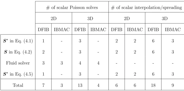
t= ∆t, we can use the second-order Runge-Kutta (RK2) scheme described in [34, 7]. In Table 1 we compare the cost of DFIB and IBMAC for the above IB scheme in terms of the number of the two cost-dominating procedures: the scalar Poisson solver which costs
O(NdlogN) using FFT on the periodic domain, where d ∈ {2,3} is the spatial dimension, and spreading/interpolation of a scalar field between the Eulerian grid and the Lagrangian mesh which costs O(M). In summary, DFIB is only more expensive than IBMAC by 4 scalar Poisson solves for two-dimensional (2D) problems, and is more expensive by 9 scalar Poisson solves and 9 scalar interpolation and spreading for three dimensional (3D) problems. Therefore, the DFIB method is about two times slower than IBMAC per time step in 3D. We point out that if the RK2 scheme [34, 7] is employed rather than the scheme above, then we can save one interpolation step per time step, but the fluid equations need to be solved twice.
5. Numerical Results
# of scalar Poisson solves # of scalar interpolation/spreading
2D 3D 2D 3D
DFIB IBMAC DFIB IBMAC DFIB IBMAC DFIB IBMAC
S? in Eq. (4.1) 1 - 3 - 2 2 6 3
S in Eq. (4.2) 2 - 3 - 2 2 6 3
Fluid solver 3 3 4 4 - - -
-S? in Eq. (4.5) 1 - 3 - 2 2 6 3
Total 7 3 13 4 6 6 18 9
Table 1: Cost of DFIB versus IBMAC in terms of the number of scalar Poisson solves and
interpola-tion/spreading of a scalar from/to the Eulerian grid.
immersed boundary. This has the effect that second-order convergence in the fluid velocity
u and the Lagrangian deformation map X can be achieved [19]. In the second set of tests, we compare volume conservation in 2D,i.e., area conservation of DFIB and IBMAC by ap-plying them to a circular membrane under tension, and we discuss the connection between area conservation and the choice of Lagrangian marker spacing relative to the Eulerian grid size. In the third set of computations, we apply the DFIB method to a problem in which a 2D elastic membrane actively evolves in a parametrically-forced system. In the last set of numerical experiments, we extend the surface tension problem to 3D, and compare volume conservation of DFIB with that of IBMAC.
5.1. A thin elastic membrane with surface tension in 2D
gen-erally only first order even if the discretization is carried out with second-order accuracy. To achieve the expected rate of convergence, we consider problems with solutions that possess sufficient smoothness.
As a simple benchmark problem with a sufficiently smooth continuum solution we con-sider a thin elastic membrane that deforms in response to surface tension only. Suppose that the elastic interface Γ is discretized by a collection of Lagrangian markersX={X1, . . . ,XM}. The discrete elastic energy functional associated with the surface tension of the membrane is the total (polygonal) arc-length of the interface [21],
E[X1, . . . ,XM] =γ M
X
m=1
|Xm−Xm−1|, (5.1)
where X0 = XM and γ is the surface tension constant (energy per unit length). The Lagrangian force generated by the energy functional at the marker Xm is
Fm∆s=−
∂E ∂Xm
=γ
Xm+1−Xm |Xm+1−Xm|
− Xm−Xm−1
|Xm−Xm−1|
. (5.2)
In our tests, we set the initial configuration of the membrane to be the ellipse
X(s,0) =L·
1 2+
5
28cos(s), 1 2 +
7
20sin(s)
, s∈[0,2π]. (5.3)
The Eulerian fluid domain Ω = [0, L]2 is discretized by a uniform N ×N Cartesian grid
with meshwidth h= L
N in each direction. The elastic interface Γ is discretized by a uniform Lagrangian mesh of size M = dπNe in the Lagrangian variable s, so that the Lagrangian markersX ={X1, . . . ,XM}are physically separated by a distance of approximately h2 in the equilibrium circular configuration. In all of our tests, we set L = 5, ρ = 1, γ = 1, µ = 0.1. The time step size is chosen to be ∆t = h
2 to ensure the stability of all simulations up to
t= 20 when the elastic interface is empirically observed to be in equilibrium.
We denote byuN(t) the computed fluid velocity field and byI2N→N a restriction operator from the finer grid of size 2N ×2N to the coarser grid of size N ×N. The discrete lp-norm of the successive error in the velocity component ui is defined by
εNp,u,i(t) =uNi (t)− I2N
→Nu2N i (t)
p. (5.4)
computation only) from the computed markers using periodic cubic splines after each time step, and compute the lp-norm error of X based on a collection of M0 uniformly sampled markersXe from the reparametrized interface, that is,
εNp,X(t) =
Xe
N(t)−
e
X2N(t)
p, (5.5)
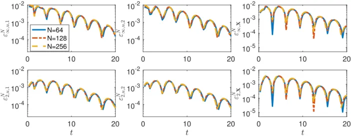
whereM0 does not change with N. We emphasize that the resampled markers are only used to compute the error norm and are discarded after each time step. In Fig. 2 the successive
l∞-norm andl2-norm errors of thex, y-component of the fluid velocity and of the deformation
map are plotted as a function of time from t = 0 to t = 20 for grid resolution N = 64,128 and 256. The number of resampled markers for computing εN
p,X(t) is M
0 = 128. To clearly
visualize that second-order convergence is achieved by our scheme, we multiply the computed errors for the finer grid resolutionN = 128 and 256 by a factor of 4 and 42 respectively, and
plot them along with errors for the coarser grid resolutionN = 64 in Fig. 2. The observation that all three error curves almost align with each other (as shown in Fig. 2) confirms that second-order convergence in u and X is achieved.
5.2. Area conservation and IB marker spacing
As an immediate consequence of fluid incompressibility, the volume enclosed by a closed immersed boundary should be exactly conserved as it deforms and moves with the fluid. However, it is observed that even in the simplest scenario of a pressurized membrane in its circular equilibrium configuration [17], the volume error of an IB method with conventional interpolation and spreading systematically grows at a rate proportional to the pressure jump across the elastic interface [35]. In this set of tests, we demonstrate that, the “volume” or area enclosed by a 2D membrane is well-conserved by the DFIB method when the Lagrangian interface is sufficiently resolved.
We follow the same problem setup as in the test described in [17]. A thin elastic membrane
X(s, t), initially in a circular equilibrium configuration,
X(s,0) =
1 2 +
1
4cos(s), 1 2+
1 4sin(s)
, s ∈[0,2π], (5.6)
0 10 20 10-4
10-3 10-2
0 10 20
10-4 10-3 10-2
0 10 20
10-4 10-3 10-2
0 10 20
10-4 10-3 10-2
0 10 20
10-5 10-4 10-3 10-2
0 10 20
10-5 10-4 10-3 10-2
N=64 N=128
N=256
Fig. 2: Rescaledl∞-norm (top panel) andl2-norm (bottom panel) errors of thex, y-component of the fluid
velocity defined by Eq. (5.4), and errors of the Lagrangian deformation map defined by Eq. (5.5) for the
2D surface tension problem are plotted as a function of time from t = 0 to t = 20. The left and middle
columns show errors of the fluid velocity components and the right column shows errors of the Lagrangian
deformation map. The Eulerian grid sizes are N = 64,128,256 and the corresponding Lagrangian mesh
sizes are M = 202,403,805, so that the spacing between two Lagrangian markers is kept at a distance of
approximately h
2 in the equilibrium configuration. For the finer grid resolutionN = 128,256, the errors in
each norm are multiplied by a factor of 4 and 42 respectively. After rescaling, the error curves of the finer
grid resolution almost align with the error curves of grid resolution N = 64, which indeed confirms that
second-order convergence inu andX is achieved. For this set of computations, we use theC3 6-point IB
Lagrangian force density on the interface is described by
F(s, t) = κ∂
2X
∂s2 , (5.7)
in which κ is the uniform stiffness coefficient. The elastic membrane is discretized by a uniform Lagrangian mesh of M points in the variable s. We approximate the Lagrangian force density by
Fm =
κ
(∆s)2 (Xm+1−2Xm+Xm−1), (5.8)
which corresponds to a collection of Lagrangian markers connected by linear springs of zero rest length with stiffness κ. For this problem, since the elastic interface is initialized in the equilibrium configuration with zero background flow, any spurious fluid velocity and area loss incurred in the simulation are regarded as numerical errors.
In our simulations, we set ρ= 1, µ= 0.1, κ= 1. The size of the Eulerian grid is fixed at 128×128 with meshwidthh= 1281 . The size of the Lagrangian meshM is chosen so that two adjacent Lagrangian markers are separated by a physical distance of hs in the equilibrium configuration, that is, M ≈ 2πR/hs, where R is the radius of the circular membrane. In addition to the Lagrangian markers, we also include a dense collection of passive tracers withNtracer = 20M to address the limiting case of moving the entire interface. These tracers
are initially in the same configuration as the circular membrane in Eq. (5.6), and they move passively with the interpolated velocity according to Eqs. (4.1) and (4.5). The time step size is set to be ∆t = h4 for stability. In all computations, we use theC3 6-point IB kernel φnew6h
to form the regularized delta function δh.
In Fig. 3 we compare the computational results of DFIB with those of IBMAC for different
hs = 4h, 2h, hand h2 (from left to right in Fig. 3). Each subplot of Fig. 3 shows a magnified view of the same arc of the circular interface along with its nearby spurious fluid velocity field. The interface represented by the Lagrangian markers X(t = 1) is shown in red and the initial configuration X(t = 0) is shown in the blue curve. The interface represented by the passive tracers Xtracer(t = 1) is shown in the yellow curve. In the first column of Fig. 3
in which hs = 4h, we see that the maximum spurious velocity kuk∞ of IBMAC is of the
wiggly pattern in the passive tracers. As the the Lagrangian mesh is refined gradually from
hs = 4h to h2 (from left to right in Fig. 3), we see that kuk∞ decreases from 10−3 to 10−7 in
the DFIB method, whereas kuk∞ stops improving around 10−4 in IBMAC. Moreover, in the
columns where hs = 2h, h, h2, we see a clear global pattern in the spurious velocity field in IBMAC, while the spurious velocity field of DFIB appears to be much smaller in magnitude and random in pattern.
We define the normalized area error with respect to the initial configuration
∆A(t;X) := |A(t;X)−A(0;X)|
A(0;X) , (5.9)
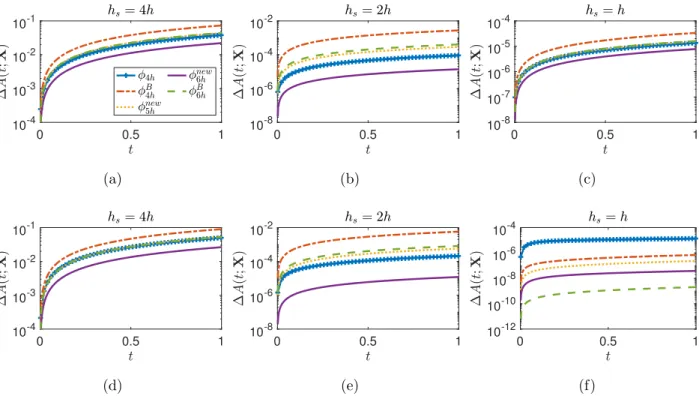
where the area enclosed by the Lagrangian markers A(t;X) is approximated by the area of the polygon formed by the Lagrangian markers X = {X1, . . . ,XM} at time t. Fig. 4 and Fig. 5 show the normalized area errors defined by Eq. (5.9) for DFIB and IBMAC with different choices of the IB kernels: φ4h ∈C1, φ4Bh ∈C2, φnew5h ∈C3,φnew6h ∈C3 andφB6h ∈C4. For the coarse Lagrangian marker spacings, for example, when hs = 2h, 4h, the area errors for IBMAC and DFIB have similar orders of magnitude (compare Fig. 4a, 4b to Fig. 4d, 4e). As the Lagrangian marker spacing is reduced from 2htoh, we see a decrease in ∆A(t;X) for IBMAC by approximately a factor of 10 (see Fig. 4b, 4c) for all the IB kernels we consider in this set of tests. In contrast, the area errors for DFIB improve by at least a factor of 103 for
the IB kernels that are at leastC2(see Fig. 4e, 4f), and in the best scenario, ∆A(t;X) forφB 6h
decreases from 10−4 to 10−9. Moreover, as the Lagrangian mesh is refined fromh to h 8, area
errors for DFIB keep improving, even approaching the machine epsilon in double precision for φB
6h at hs = h4,h8 and for φnew6h at hs = h8 (see Fig. 5e, 5f). For a moderate Lagrangian marker spacing, such ashs =hand h2, area errors for DFIB are several orders of magnitude smaller than those of IBMAC. On the other hand, area errors for IBMAC stop improving around 10−5 forh
s ≤h, no matter how densely the Lagrangian mesh is refined (see Fig. 4c, 5c). We remark that the smoothness of the IB kernel appears to play an important role in volume conservation of DFIB. In this study DFIB achieves the best volume conservation result for hs ≤ h with φB6h, and this kernel also has the highest regularity of the kernel functions considered in this work.
hs= 4h
0.25 0.35
0.6 0.7
kuk∞ = 7.33e-03
hs= 2h
0.25 0.35
0.6 0.7
kuk∞= 2.95e-04
hs=h
0.25 0.35
0.6 0.7
kuk∞ = 2.77e-04
hs= 0.5h
0.25 0.35
0.6 0.7
kuk∞ = 2.76e-04
X(t= 0) X(t= 1) Xtracer(t= 1)
(a) IBMAC
hs= 4h
0.25 0.35
0.6 0.7 k
uk∞ = 8.09e-03
hs= 2h
0.25 0.35
0.6 0.7 k
uk∞= 1.20e-04
hs=h
0.25 0.35
0.6 0.7 k
uk∞ = 1.12e-05
hs= 0.5h
0.25 0.35
0.6 0.7 k
uk∞ = 8.57e-07
X(t= 0) X(t= 1) Xtracer(t= 1)
(b) DFIB
Fig. 3: A magnified view of the quasi-static circular membrane and its nearby spurious velocity field for
different Lagrangian mesh spacinghs= 4h,2h, hand h2, as indicated below each figure panel, while keeping
h= 1281 fixed. The top panel (a) shows the computational results from IBMAC, and the bottom panel (b)
shows the results from DFIB. The interface represented by the Lagrangian markers X(t = 1) is shown in
red, the initial configuration X(t = 0) is shown in blue, and the interface represented by Ntracer = 20M
passive tracers is shown in yellow, whereM is the number of Lagrangian markers. The time step size is set
to be ∆t=h4 for stability. In the above computations, theC36-point IB kernelφnew
6h is used in IBMAC and
error. The first source of error is the time-stepping error from the temporal integrator, which is relatively small in the quasi-static circle test. The second source of area loss comes from discretizing the continuous curve (circle) as a polygon whose vertices are the IB markers. This kind of error can be substantially reduced by using a high-order representation of the interface, such as a periodic cubic spline. We define a normalized area error with respect to the true initial area of the interface Atrue by using the tracers,
∆A(t;Xtracer) :=
|A(t;Xtracer)−Atrue|
Atrue
, (5.10)
where we compute A(t;Xtracer) via exact integration of the cubic spline interpolant. Fig. 6
shows that the area enclosed by the passive tracers using the cubic spline approximation is far more accurately preserved than the polygonal approximation. Furthermore, the area error approaches zero as the discretization of the tracer interface is refined, even if the marker and grid spacings are held fixed, as shown in Fig. 6. Indeed, the area of the spline interpolant through the tracers of spacing hs/20 = h/20 is conserved to the machine epsilon in double precision.
It is well-known that the traditional IB method produces non-smooth surface tractions, and a number of improvements have been proposed [11, 44, 45, 39, 29]. Somewhat unex-pectedly, the divergence-free force spreading used in our DFIB method proposed here offers smoother and more accurate tractions without any post-processing such as filtering [11]. This is inherently linked to the reduced spurious flows compared to traditional methods [39]. In Fig. 7, we compare the errors of the tangential and normal components of F(s, t= 1) for DFIB and IBMAC for the quasi-static circle problem. We observe that the DFIB method dramatically improves the accuracy of Lagrangian forces by only refining the Lagrangian mesh, keeping the Eulerian grid fixed. By contrast, in the IBMAC method, the tractions do not improve as the Lagrangian grid is refined.
5.3. A thin elastic membrane with parametric resonance in 2D
0 0.5 1 10-4
10-3 10-2 10-1
(a)
0 0.5 1
10-8 10-6 10-4 10-2
(b)
0 0.5 1
10-8 10-7 10-6 10-5 10-4
(c)
0 0.5 1
10-4 10-3 10-2 10-1
(d)
0 0.5 1
10-8 10-6 10-4 10-2
(e)
0 0.5 1
10-12 10-10 10-8 10-6 10-4
(f)
Fig. 4: Normalized area errors of the pressurized circular membrane (relative to the initial area, see (5.9))
simulated by IBMAC (top panel) and DFIB (bottom panel) with the IB kernels: φ4h ∈ C1, φB4h ∈ C2,
φnew
5h ∈C3,φnew6h ∈C3andφB6h∈C4, and with Lagrangian marker spacingshs∈ {4h,2h, h}indicated above
0 0.5 1 10-8 10-7 10-6 10-5 10-4 (a)
0 0.5 1
10-8 10-7 10-6 10-5 10-4 (b)
0 0.5 1
10-8 10-7 10-6 10-5 10-4 (c)
0 0.5 1
10-16 10-14 10-12 10-10 10-8 10-6 (d)
0 0.5 1
10-16 10-14 10-12 10-10 10-8 10-6 (e)
0 0.5 1
10-16 10-14 10-12 10-10 10-8 10-6 (f)
Fig. 5: Normalized area errors of the pressurized circular membrane (relative to the initial area, see (5.9))
simulated by IBMAC (top panel) and DFIB (bottom panel) with the IB kernels: φ4h ∈ C1, φB4h ∈ C2,
φnew
5h ∈C3,φ6newh ∈C3 andφB6h∈C4, and with Lagrangian marker spacings,hs∈h2,h4,h8 indicated above
each figure panel. As the Lagrangian mesh is refined, area errors for DFIB keep improving, even approaching
the machine precision forφB6h aths=h4,h8 and forφnew6h aths=h8.
0 0.5 1
10-16 10-14 10-12 10-10 10-8 10-6 10-4
0 0.5 1
10-16 10-14 10-12 10-10 10-8 10-6 10-4
Fig. 6: Normalized area errors of the interface enclosed by the tracers that move passively with the
inter-polated velocity of the DFIB method (relative to the true area of the circle, see Eq. (5.10)). The initial
configuration of the interface is given by Eq. (5.6), andφnew
6h is used for this computation. From left to right,
the Lagrangian marker spacing is hs∈h,h2 , as shown in each figure panel. In each case, the area error
enclosed by the tracers is computed for tracer resolutionNtracer=M and 20M in two ways: (1) by the area
of the polygon formed by the tracers, and (2) by the exact integration of the cubic spline interpolant of the
0 /4 /2 10-16
10-14 10-12 10-10 10-8 10-6 10-4
0 /4 /2
10-10 10-8 10-6 10-4 10-2
(a) DFIB
0 /4 /2
10-16 10-14 10-12 10-10 10-8 10-6 10-4
0 /4 /2
10-10 10-8 10-6 10-4 10-2
(b) IBMAC
Fig. 7: Normalized errors of the normal Fr (top panels) and tangentialFθ (bottom panels) components of
the Lagrangian force F(s, t= 1) of the circular membrane for s∈[0,π
2]. The computations are performed
using DFIB (left panels) and IBMAC (right panels) withφnew
6h , and with Lagrangian marker spacingshs∈
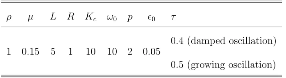
ρ µ L R Kc ω0 p 0 τ
1 0.15 5 1 10 10 2 0.05
0.4 (damped oscillation)
0.5 (growing oscillation)
Table 2: Parameters used to simulate the motion of the 2D membrane with parametric resonance.
simple prototype problem for active fluid-structure interaction is a thin elastic membrane that dynamically evolves in a fluid in response to elastic forcing with periodic variation in the stiffness parameter [6, 23], that is,
F(s, t) = κ(t)∂
2X
∂s2 , (5.11)
where κ(t) is a periodic time-dependent stiffness coefficient of the form
κ(t) =Kc(1 + 2τsin(ω0t)). (5.12)
It is quite remarkable that such a purely temporal parameter variation can result in the emergence of spatial patterns, but that is indeed the case. We assume that the immersed structure is initially in a configuration that has a small-amplitude perturbation from a circle of radius R,
X(s,0) =R(1 +0cos(ps)) rˆ(s), (5.13)
whererˆ(s) denotes the position vector pointing radially from the origin. For certain choices of parameters, the perturbed mode in the initial configuration may resonate with the driving frequency ω0 in the periodic forcing, leading to large-amplitude oscillatory motion in the
membrane. The stability of the parametric resonance has been studied in the IB framework using Floquet linear stability analysis for a thin elastic membrane in 2D [6, 23], and recently for an elastic shell in 3D [24]. Motivated by the linear stability analysis of [6, 23], we consider two sets of parameters listed in Table 2 for our simulations. The first set of parameters with
1 4 1
4
t = 0 t = 4.5
0 1 2 3 4 5 6 7 8 9 10
-0.05 0 0.05
(a)
1 4
1 4
t = 0 t=2 t=9.5 t = 25
0 5 10 15 20 25
-0.5 -0.3 -0.1 0.1 0.3 0.5
unstable
stable
(b)
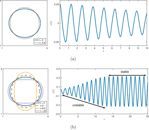
Fig. 8: Left panel: snapshots of the 2D membrane with parametric resonance. Right panel: the
time-dependent amplitude(t) of the perturbed mode in Eq. (5.14). (a) Damped oscillation (b) Growing
The computational domain Ω = [0, L]2 is discretized by a 128×128 uniform Cartesian
grid with meshwidth h = 128L . The number of Lagrangian markers is determined so that the distance between the Lagrangian markers is hs ≈ h2 in the initial configuration. The discretization of the Lagrangian force density Eq. (5.11) is constructed in the same way as Eq. (5.8). The time step size is ∆t = h
10 to ensure the stability of computation. On the left
panel of Fig. 8 we show snapshots of the membrane configuration for each case, and on the right panel we plot the time-dependent amplitude (t) of the ansatz
X(s, t) = R(1 +(t) cos(ps))rˆ(s) (5.14)
by applying the FFT to the Lagrangian marker positions X. In the case of growing os-cillation (Fig. 8b), the amplitude of the perturbed mode increases from 0.05 to 0.3 until nonlinearities eventually stabilize the growing mode and the membrane starts to oscillate at a fixed amplitude.
We next give a direct comparison of area conservation of IBModified (with φcos 4h [35]), IBMAC, and DFIB with the IB kernels φ4h ∈ C1, φB4h ∈ C2, φnew5h ∈ C3, φnew6h ∈ C3 and
φB
6h ∈ C4. In this test, the area enclosed the Lagrangian markers is computed by the cubic spline approximation discussed in Sec. 5.2. In Fig. 9 and Fig. 10 we show time-dependent area errors enclosed by the parametric membrane for the damped-oscillation and the growing-amplitude cases respectively. For the damped-oscillation case (Fig. 9), we see that area errors for DFIB are at least two orders of magnitude smaller than those of IBMAC and IBModified for IB kernels that are at leastC2. The volume conservation of IBModified and IBMAC was
not directly compared in the previous work [17], but it was anticipated that they are similar. In our comparison, we find that IBModified is only slightly better than IBMAC in volume conservation, yet IBMAC is much simpler to use in practice.
In this set of tests, the choice of IB kernel also plays a role in affecting area conservation. In particular, the area errors for DFIB using φnew
6h and φB6h are smaller than those of φB4h and φnew
5h by approximately one order of magnitude. Additionally, the error curves of DFIB with φnew
6h and φB6h remain oscillating below 10
−7 while apparent growth of error in time is
observed with φB
collection of Lagrangian markers, the time-stepping error in this example can be observed by considering a dense collection of tracers with different time step sizes. With Ntracer = 4M,
we first confirm that the area error of the tracer interface cannot be reduced by further including more tracers, but as we reduce the time step size ∆t∈h
10, h 20,
h
40 , we observe an
improvement in the area error, as shown in the bottom panel of Fig. 9. The improvements in area conservation of DFIB is consistently more than 104 times over IBCollocated and about
103 times over IBMAC. Similar results are obtained for the growing-amplitude case (see Fig. 10) except that the parametrically-unstable membrane has experienced some area loss due to the growing-amplitude oscillation before its motion is stabilized by the nonlinearities.
5.4. A 3D thin elastic membrane with surface tension
In our final test problem, we examine volume conservation of the DFIB method by ex-tending the surface tension problem to 3D. We consider in 3D a thin elastic membrane that is initially in its spherical equilibrium configuration. The spherical surface of the mem-brane is discretized by a triangulation consisting of approximately equilateral triangles with edge length approximately equal to hs, constructed from successive refinement of a regular icosahedron by splitting each facet into four smaller equilateral triangles and projecting the vertices onto the sphere to form the refined mesh (see Fig. 11 for the first two levels of refine-ment). We use {X1,X2, . . . ,XM} and {T1,T2, . . . ,TP} to denote the vertices (Lagrangian markers) and the triangular facets of the mesh respectively. The generalization of discrete elastic energy functional of surface tension in 3D is the product of surface tension constant
γ (energy per unit area) and the total surface area of the triangular mesh [22], that is,
E[X1, . . .XM] =γ P
X
p=1
|Tp|, (5.15)
where |Tp| is the area of the pth triangle. The Lagrangian force Fk∆s at the kth vertex is minus the partial derivative of E[X1, . . . ,XM] with respect to Xk,
Fk∆s=−
∂E ∂Xk
=−γ X
l∈nbor(k)
∂|Tl|
∂Xk
0 1 2 3 4 5 6 7 8 9 10 10-6
10-4 10-2
0 2 4 6 8 10
10-10 10-8 10-6
8.5 9
8 10
10-4
0 1 2 3 4 5 6 7 8 9 10
10-13 10-11 10-9 10-7
Fig. 9: Top and middle panels: normalized area errors ∆A(t;X) (relative to the initial area, see (5.9)) of
the 2D parametric membrane undergoing damped oscillatory motion (corresponding to the motion shown
in Fig. 8a) are plotted on the semi-log scale. The area enclosed by the markers is computed by the exact
integration of a cubic spline approximation. The computations are performed using IBMAC and DFIB with
the IB kernels: φ4h∈C1,φB4h∈C 2, φnew
5h ∈C 3,φnew
6h ∈C
3and φB 6h ∈C
4, and IBModified withφcos 4h ∈C
1.
The top panel shows area errors for IBMAC and IBModified, and the middle panel shows area errors for
DFIB. The bottom panel shows improvement in area errors (relative to the true area of the ellipse, see (5.10))
enclosed by the interface ofNtracer= 4M tracers by reducing the time step size: ∆t∈
h 10,
h 20,
0 2 4 6 8 10 12 14 16 10-6
10-4 10-2
0 2 4 6 8 10 12 14 16 10-9
10-7 10-5
1
2 10
-5
16 17 18 19 20 21 22 23 24 25
10-9 10-7 10-5
Fig. 10: Normalized area errors ∆A(t;X) of the 2D parametric membrane undergoing growing-amplitude
oscillatory motion (corresponding to the motion shown in Fig. 8b) are plotted on the semi-log scale, as done
in Fig. 9 for damped motion. The computations are performed using IBMAC and DFIB with the IB kernels:
φ4h∈C1,φB4h ∈C 2, φnew
5h ∈C 3,φnew
6h ∈C
3 andφB 6h ∈C
4, and IBModified with φcos 4h ∈C
1. The top panel
shows area errors for IBMAC and IBModified, the middle panel shows the area errors for DFIB fort= 0 to
where nbor(k) denotes the set of indices of triangles that share Xk as a vertex3. Each component of the term ∂|Tl|/∂Xk in Eq. (5.16) can be computed analytically [22],
∂|Tl|
∂Xk α = ∂ ∂Xk,α 1 2
(Xk−X
0
k)×(X0k−X 00 k) = 1 2
(X0k−X00k)×nˆl
α
, α= 1,2,3, (5.17)
whereXk, X 0 k, X
00
kdenote the three vertices of the triangleTlordered in the counterclockwise direction and nˆ is the unit outward normal vector of Tl.
The computation is performed in the periodic box Ω = [0,1]3 with Eulerian meshwidth
h = 1281 using DFIB with φnew6h . For the quasi-static test, the initial fluid velocity is set to be zero, and for the dynamic test, we set u(x,0) = (0, sin(4πx), 0). In the computational results shown in Fig. 12, the spherical membrane is discretized by triangulation (as shown in Fig. 11) with 5 successive levels of refinement from the regular icosahedron (Fig. 11a), which results in a triangular mesh with M = 10242 vertices and P = 20480 facets. The radius of the spherical membrane is set to be R ≈ 0.1 which corresponds to hs ≈ h2. The remaining parameters in the computation are ρ = 1, µ = 0.05, γ = 1 and the time step size ∆t = h4. In Fig. 12 we show snapshots of the 3D elastic membrane at t = 0, 321 , 14
and 12 for the dynamic case. The elastic interface is instantaneously deformed by the fluid flow in the y-direction, and due to surface tension, the membrane eventually relaxes back to the spherical equilibrium configuration. Colored markers that move passively with the divergence-free interpolated fluid velocity are added for visualizing the fluid flow in the vicinity of the interface.
The volume enclosed by the triangular surface mesh is approximated by the total volume of tetrahedra formed by each facet and one common reference point (e.g. the origin) using the scalar triple product. To study volume conservation of the DFIB method in 3D, we compare the normalized volume error defined by
∆V(t;X) := |Vol(t;X)−Vol(0;X)|
Vol(0;X) (5.18)
3Here ∆sis the Lagrangian area associated with each node andF
k is the Lagrangian force density with
respect to Lagrangian area, but note that we do not needFk and ∆sseparately; only their product is used
using IBMAC and DFIB with hs = h,h2,h4, which correspond to triangular meshes with 4,5,6 levels of refinement from the regular icosahedron respectively. For the quasi-static case (Fig. 13a), volume errors for DFIB are at least 2 orders of magnitude smaller than those of IBMAC. Further, volume errors for DFIB keep decreasing as the Lagrangian mesh is refined fromhs=hto h4. For the dynamic case (Fig. 13b), both methods suffer a significant amount of volume loss arising from the rapid deformation at the beginning of simulation. The volume error of DFIB withhs =his similar to those of IBMAC in magnitude, but the volume error of DFIB decreases as the Lagrangian mesh is refined forhs = h2,h4. It appears that the behavior of volume error changes in nature from hs =h to h2, which coincides with the conventional recommendation that the best choice of Lagrangian mesh spacing in the IB method ishs= h2 in practice. Similar to the two sources of error that contribute to the area loss in 2D, the volume error observed in Fig. 13 can also be explained by contribution from the time-stepping error, and the volume loss due to only moving the vertices (Lagrangian markers) that constitute the triangular mesh. This kind of error in volume conservation decreases as the discretization of the surface is refined, even on a fixed Eulerian grid (as shown in Fig. 13). Finally, we remark that the improvement in volume conservation does not seem to be as substantial as the improvement in area conservation in 2D. We suspect that this may be attributed to the larger approximation error in computing the volume using the tetrahedral approximation (after the triangular mesh is deformed), whereas in two dimensions we use a higher-order representation of the interface (cubic splines). Nevertheless, the reduction in volume error from the Lagrangian mesh-refinement experiments indeed confirms that the DFIB method can generally achieve better volume conservation if the immersed boundary is sufficiently resolved (hs≤ h2).
6. Conclusions
corre-(a) (b) (c)
Fig. 11: Triangulation of a spherical surface mesh via refinement of a regular icosahedron. (a) Regular
icosahedron (b) Refined mesh after one level of refinement (c) Refined mesh after two levels of refinement.
(a)t= 0 (b)t= 321
(c) t= 14 (d)t= 12
Fig. 12: Deformation of a 3D elastic membrane immersed in a viscous fluid with initial velocityu(x, t) =
(0, sin(4πx), 0) at t= 0,321,14 and 12. The computation is performed using DFIB withφnew6h in the periodic
box Ω = [0,1]3with Eulerian meshwidthh=1281 . The elastic membrane, initially in spherical configuration
with radiusR≈0.1, is discretized by a triangular surface mesh withM = 10242 vertices andP= 20480 facets
so thaths = h2 in the initial configuration. Colored markers that move passively with the divergence-free
0 0.1 0.2 0.3 0.4 0.5 10-11
10-9 10-7 10-5 10-3
(a) Quasi-static test
0 0.1 0.2 0.3 0.4 0.5
10-7 10-5 10-3
(b) Dynamic test
Fig. 13: Normalized volume error ∆V(t;X) of a 3D elastic membrane using IBMAC and DFIB withhs=
h,h 2,
h
4, where h= 1
128. For (a) the quasi-static test, ∆V(t,X) of DFIB decreases with mesh refinement,
while there is no improvement in volume error for IBMAC. For (b) the dynamic test, the volume error in
DFIB remains (almost) steady in time forhs= h2,h4 as the membrane rests, whereas we see no substantial
improvement in volume conservation with mesh refinement for IBMAC, and the volume loss keeps increasing
in time. For this set of computations, theC3 6-point kernelφnew
6h is used.
sponding force-spreading operator is constructed to be the adjoint of velocity interpolation so that energy is preserved in the interaction between the fluid and the immersed bound-ary. Both the new interpolation and spreading schemes require solutions of discrete vector Poisson equations which can be efficiently solved by a variety of algorithms. The transfer of information from the Eulerian grid to the Lagrangian mesh (and vice versa) is performed using ∇δh on the edge-centered staggered grid E. We have found that volume conservation of DFIB improves with the smoothness of the IB kernel used to construct δh, and we have numerically tested that IB kernels that are at least C2 are good candidate kernels that can
be used to construct the regularized delta function in the DFIB method.
a continuous normal derivative of the tangential velocity across the immersed boundary. The highlight of the DFIB is its capability of substantially reducing volume error in the immersed structure as it moves and deforms in the process of fluid-structure interaction. Through numerical simulations of quasi-static and dynamic membranes, we have confirmed that the DFIB method improves volume conservation by several orders of magnitude com-pared to IBMAC and IBModified. Furthermore, owing to the divergence-free nature of its velocity interpolation, the DFIB method reduces volume error with Lagrangian mesh re-finement while keeping the Eulerian grid fixed. A similar rere-finement study would not yield improved volume conservation when using the conventional IB method. Although the nu-merical examples considered in this paper only involve thin elastic structures, we note that the DFIB method can also be directly applied to model thick elastic structures without any modification to the method, other than representing the thick elastic structure by a curvi-linear mesh of Lagrangian points [19, 10, 18, 4]. We also remark that the current version of the DFIB method is accompanied with a single-fluid Navier-Stokes fluid solver. This is not a fundamental limitation in our approach, and as a direction of future research, the DFIB method may be extended to work with variable-viscosity and variable-density fluid solvers [9].
Unlike other improved IB methods that either use non-standard finite-difference oper-ators (IBModified [35]) that complicate the implementation of the fluid solver, or rely on analytically-computed correction terms (IIM [28, 27] or Blob-Projection method [5]) that may not be readily accessible in many applications, the DFIB method is generally applica-ble, and it is straightforward to implement in both 2D and 3D from an existing IB code that is based on the staggered-grid discretization. Moreover, the additional costs of performing the new interpolation and spreading do not increase the overall complexity of computation and are modest compared to the existing IB methods.


![Fig. 7: Normalized errors of the normal F r (top panels) and tangential F θ (bottom panels) components of the Lagrangian force F(s, t = 1) of the circular membrane for s ∈ [0, π 2 ]](https://thumb-us.123doks.com/thumbv2/123dok_us/8295635.2196880/29.918.106.811.288.789/normalized-errors-normal-tangential-components-lagrangian-circular-membrane.webp)