Graph based pattern discovery in protein structures

(1)

Graph Based Pattern Discovery in Protein Structures

by Jun Huan

A dissertation submitted to the faculty of the University of North Carolina at Chapel Hill in partial fulfillment of the requirements for the degree of Doctor of Philosophy in the Department of Computer Science.

Chapel Hill 2006

Approved by, Advisor: Wei Wang Reader: Nikolay V. Dokholyan

(2)

c 2006 Jun Huan

(3)

ABSTRACT

JUN HUAN: Graph Based Pattern Discovery in Protein Structures. (Under the direction of Jan Prins and Wei Wang.)

The rapidly growing body of 3D protein structure data provides new opportunities to study the relation between protein structure and protein function. Local structure pattern of proteins has been the focus of recent efforts to link structural features found in proteins to protein function. In addition, structure patterns have demonstrated values in applica-tions such as predicting protein-protein interaction, engineering proteins, and designing novel medicines.

My thesis introduces graph-based representations of protein structure and new subgraph mining algorithms to identify recurring structure patterns common to a set of proteins. These techniques enable families of proteins exhibiting similar function to be analyzed for structural similarity. Previous approaches to protein local structure pattern discovery operate in a pair-wise fashion and have prohibitive computational cost when scaled to families of proteins. The graph mining strategy is robust in the face of errors in the structure, and errors in the set of proteins thought to share a function.

(4)

(5)

ACKNOWLEDGMENTS

I want to thank Jan Prins and Wei Wang, who have been my thesis co-advisors over the past four years. Jan and Wei took me into the fields of data mining and bioinformatics. Wei originally recognized the importance of frequent subgraph mining techniques, which become the main theme of this dissertation. In overcoming the difficulties of graph based protein structure analysis, Jan first realized the importance of rigorous mathematical representations of protein structures. His insightful comments shaped the current thesis. It is truly because of their effort and encouragement that I am fulfilling my long term goal of using computational method to analyzing bio-molecules. In addition, Jan and Wei encouraged me during difficult times in my Ph.D. study and helped me in writing the dissertation. Finally, I thank Jan and Wei for supporting me financially through a research assistantship over my Ph.D. study, and also for a generous travel allowance that enabled me to present my work at several conferences including ACM SIGKDD’04 and ’05, and IEEE CSB’06.

I also want to extend my thanks to my committee members for their comments and inputs during the thesis development. Alex Tropsha has been directly involved in the work of structure motif identification and functional annotation. Over years, Alex taught me how to capture a driving biological problem and to focus my research on delivering testable hypotheses for domain experts. I benefit from this research philosophy. Jack Snoeyink has been involved in nearly all aspects of the dissertation development, including but not limited to algorithm design, experimental design, and writing reports. Among many things that I learned from Jack, I emphasize the passion for solving intriguing mathematical problems and the skills of writing concise technical reports. Nikolay Dokholyan introduced me the complex protein structure evolutionary problem. He shared his vision and encouraged me all the way through my study of the problem with him.

(6)

to work on structure pattern discovery in nuclear binding proteins. I thank Todd for offering me a summer research position in his group for working on genome evolution.

I also want to thank all the students that I worked with. They are my colleagues, paper coauthors, friends, and mentors. I listed their names in a rough chronological order: Deepak Bandyopadhyay, Ruchir Shah (UNC School of Pharmacy), Angliana Washington, Jinze Liu, Xiang Zhang, Xueyi Wang, and David Williams.

I want to thank all the students in the motifSpace group in UNC Computer Science De-partment: Kiran Sidhu, Tao Xie, and Jingdan Zhang; I want to thank my friends at Dr. Tropsha’s Molecular Modeling Laboratory at UNC School of Pharmacy: King Zhang, Jun Feng, Min Shen, and Yetian Chen; I also want to thank members of the computational ge-ometry group: Andrea Mantler, Andrew Leaver-Fay, Yuanxin (Leo) Liu, and David O’Brien. I thank the excellent staff of the Computer Science department at UNC Chapel Hill for their help and support. Mike Stone helped me fix my laptop several times during my Ph.D. study. Janet Jones, Tammy Pike, and Sandra Neely help me with administrative issues during my student life and being good friends.

I could not finish my Ph.D. study without financial support. I want to thank UNC General Assembly for providing my a one-year financial support. I want to thank NSF and NIH, whose grants, through PIs of Wei, Jan, Alex, and Jack, supported me.

(7)

LIST OF FIGURES

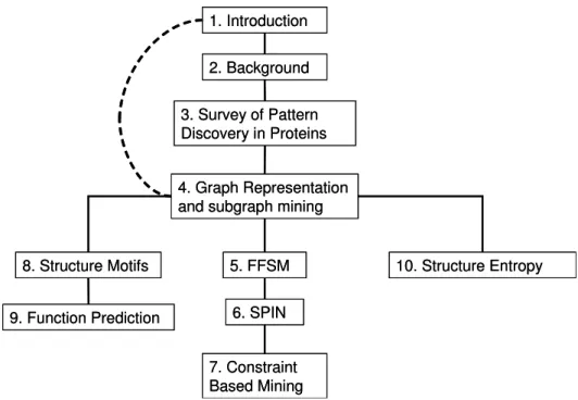
1.1 Dissertation Organization . . . 9

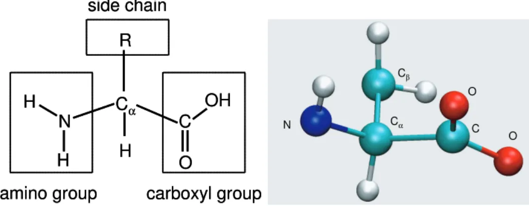
2.1 Amino Acids . . . 12

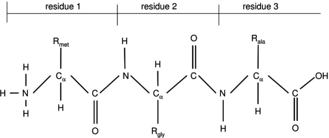
2.2 Peptide . . . 13

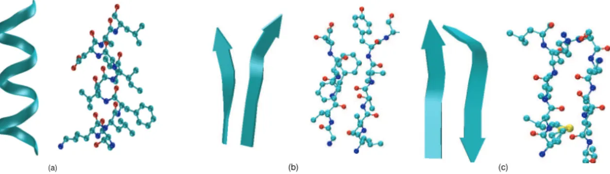
2.3 Secondary Structures . . . 14

2.4 3D Structures . . . 14

2.5 Protein Classification . . . 16

3.1 Taxonomy of Local Structure Comparison . . . 20

4.1 Example of Graphs . . . 34

4.2 Subgraph Isomorphism . . . 37

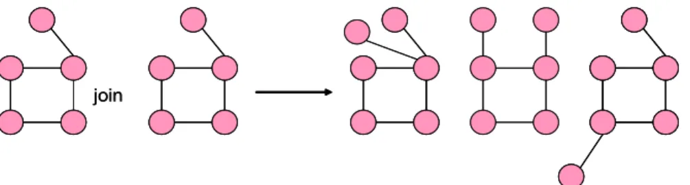
4.3 FSG Join Operation . . . 41

4.4 Graph Path Cover . . . 44

5.1 Graph Matrix Representation . . . 49

5.2 A Partial Order of Graphs . . . 50

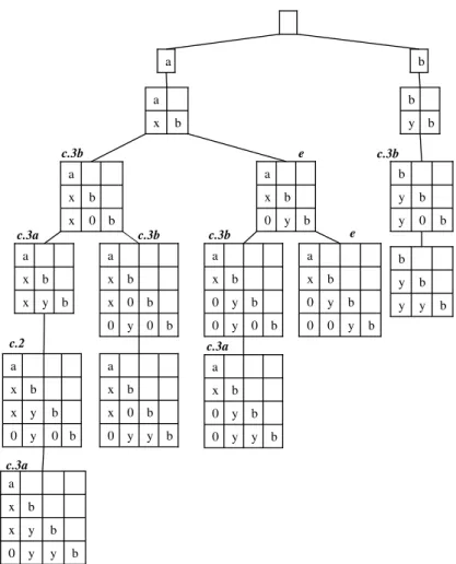
5.3 CAM Tree . . . 51

5.4 FFSM Join and Extension . . . 55

5.5 Suboptimal CAM Tree . . . 58

5.6 FFSM Performance with Synthetic Graphs I . . . 62

5.7 FFSM Performance with Synthetic Graphs II . . . 62

5.8 FFSM Performance with Chemical Structures I . . . 63

5.9 FFSM Performance with Chemical Structures II . . . 63

6.1 A sample graph database for SPIN . . . 67

(16)

6.3 Spanning trees of a graph . . . 71

6.4 Canonical Spanning Tree . . . 72

6.5 Tree based equivalence class . . . 74

6.6 Enumerating graphs in one equivalence class . . . 75

6.7 Tail shrink . . . 79

6.8 Associative external edges . . . 80

6.9 SPIN performance comparison I . . . 84

6.10 SIN performance comparison II . . . 85

6.11 SPIN performance comparison III . . . 85

6.12 SPIN performance comparison IV . . . 86

7.1 Frequent Cliques . . . 89

7.2 Graph Normalization . . . 91

7.3 CliqueHashing Algorithm Example . . . 94

7.4 CliqueHashing Algorithm Example for MultiLabeled Graphs . . . 97

8.1 Distance bins . . . 102

8.2 Voronoi diagram . . . 103

8.3 Comparing different graph representations . . . 105

8.4 Performance comparison with different graph representations . . . 105

8.5 Structure motifs for serine protease family . . . 108

8.6 Structure motifs in two protein families . . . 109

8.7 Structure pattern in FAD/NAD-linked reducatase family . . . 110

9.1 Structure Fingerprints . . . 115

9.2 Discriminating TIM Barrel Proteins . . . 116

(17)

10.2 Contact probability . . . 132

10.3 Structure entropy for the Ig Family . . . 133

10.4 Sequence and structure entropy for the Ig family . . . 134

10.5 Sequence and structure entropy corrleation . . . 135

10.6 An example structure pattern . . . 137

(18)

LIST OF TABLES

5.1 FFSM Performance with Protein Contact Maps . . . 63

6.1 SPIN synthetic data sets . . . 84

6.2 SPIN chemical data sets . . . 86

8.1 Data set in structure motif case studies . . . 107

9.1 Function inference . . . 118

9.2 Families with no new members inferred. . . 119

9.3 Families with new members inferred. . . 119

10.1 Data set in structure entropy . . . 126

10.2 Neighbor set . . . 129

10.3 Projected neighbor set . . . 130

10.4 Projected entropies . . . 131

10.5 Fold family statistics . . . 132

10.6 Linear correlation between structure and sequence entropy . . . 136

(19)

Chapter 1 Introduction

A protein is a chain of amino-acid molecules. In conditions found within a living organism, the chain of amino acids folds into a relatively stable three-dimensional arrangement known as the native structure. The native structure of a protein is a key determinant of its function [EJT04, MBHC95, OMJ+97, Ric81]. Exactly how protein function is determined by protein structure is the central question in structural biology, and computational methods to compare the structures of proteins are a vital part of research in this area.

Starting from the 3D coordinates of the atoms in a protein (as obtained by a number of experimental techniques described later), global structure comparison can determine the similarity of two complete protein structures. Global structure comparison is widely used to classify proteins into groups according to their global similarity [HS96].

However, a protein’s global structure does not always determine its function. There are well known examples of proteins with similar global structure but different functions. Con-versely, there are also examples of proteins with similar function but quite different global structure. For this reason there has been increased interest in structure pattern discovery in order to identify structural similarity between parts of proteins [FWLN94]. The goal of structure pattern discovery is to recognize conserved geometric arrangements of amino acids in protein structures, orstructure patterns.

(20)

1.1 Motivation

This section describes the factors that underscore the need for automated protein structure comparison methods. Readers with limited knowledge of proteins and protein structure may wish to read Chapter 2 for related background before proceeding further.

1.1.1 Rapidly Growing Catalogs of Protein Structure Data

Recognizing the importance of structural information, the Protein Structure Initiative (PSI, http://www.nigms.nih.gov/psi/) and other recent efforts have targeted the accurate deter-mination of all protein structures specified by genes found in sequenced genomes [CBB+_02,

TWP+98]. The result has been a rapid increase in the number of known 3D protein structures. The Protein Data Bank (PDB) [BWF+_{00]), a public on-line protein structure repository,}

con-tained more than 30,000 entries at the end of year 2005. The number of structures is growing exponentially; more than 5,000 structures were added to the PDB in 2005, about the same as the total number of protein structures added in the first four decades of protein structure determination [KBD+58].

Along with individual protein structures, the structure of certain complexes of interacting proteins are known as well. While relatively few complexes have been completely determined, there is rapidly growing information about which proteins interact. Among the proteins in yeast alone, over 14,000 binary interactions have been discovered [SSK+05]. The IntAct database records 50,559 binary interactions involving 30,497 proteins [HMPL+_{04] from many}

species. Experts believe that many more interactions remain to be identified. For example, among the proteins in yeast it is estimated that there are about 30,000 binary interactions [vMHJ+_03].

Additional types of data whose relation to protein structure is of interest are being accu-mulated as well, such as the cellular localization of proteins, the involvement of proteins in signaling, regulatory, and metabolic pathways, and post-translation structural changes in pro-teins [AM13, PBZ+_{13]. The rapidly growing body of data call for automatic computational}

tools rather than manual processing.

1.1.2 Pattern Discovery Aids Experiment Design

Protein structure comparison is part of a bioinformatics research paradigm that performs comparative analysis of biological data [SIK+_{04]. The overarching goal is to aid rational}

(21)

pattern based structure alignment, functional site identification, structure-based functional annotation, and protein evolution. A comprehensive review can be found in [JT04].

Pattern-Based Structure Alignment

Structure alignment is vital to identifying conserved residues in protein structure, to studying the evolution of protein structures, and to facilitating structure prediction. For example, through structure alignment, domain experts discover that many diverse sequences may adopt the same global structure and such information helps significantly in structure prediction [KMS00].

Multiple structure alignment has been used to identify structural commonalities among a group of proteins. Two approaches have been investigated. The first uses multiple sequence alignment to solve the difficult alignment problem and then focuses on identifying the struc-tural core of proteins. The second approach applies pairwise structure alignment iteratively in order to derive multiple structure alignment.

Leibowitz et al.first proposed a multiple structure alignment method based on recurring structure patterns [LFNW01]. In their method, multiple structure alignment is done in three steps. First, a group of common structure patterns is obtained using the geometric hashing method. Second, for each structure pattern, the occurrences of the pattern in the group of proteins are computed and aligned. Third, among many possible multiple alignments, the optimal one (one that covers the largest number of amino acid residues) is searched and used for the final multiple structure alignment.

Compared with traditional methods, pattern-based structure alignment has the following advantages [LFNW01]:

• It does not rely on multiple sequence alignment

• It handles well insertion/deletion or point mutations in protein structures

• all structures are considered simultaneously

For other pattern based structure alignment methods, see [RSKC05]

Functional Site Identification

(22)

Traditionally, functional sites are derived through expensive experimental techniques such as site-directed mutagenesis. This technique creates a modified protein in which one or more amino acids are replaced in specific locations to study the effect on protein function. However, site-directed mutagenesis studies are both labor intensive and time consuming, as there are many potential functional sites. In search of an alternative approach, more than a dozen methods based on the analysis of protein local structure have been developed [TBPT05]. All are based on the idea that functional sites in proteins with similar function may be composed of a group of specific amino acids in approximately the same geometric arrangement. The methods differ from each other in algorithmic details as described in Section 3. The essence of the approach is to identify local structure that recurs significantly among proteins with similar function.

Structure-based Functional Annotation

There is no question that knowing the function of a protein is of paramount importance in biological research. As expressed by George and his coauthors [GSB+_{05], correct function}

prediction can significantly simplify and decrease the time needed for experimental validation. However incorrect assignments may mislead experimental design and waste resources.

Protein function prediction has been investigated by recognizing the similarity of a protein with unknown function to one that has a known function where similarity can be determined at the sequence level [WSO01], the expression level [DLS00], and at the level of the gene’s chromosome location [OMD+99].

In structure based function annotation, investigators focus on assigning function to pro-tein structures by recognizing structural similarity. Compared to sequence-based function assignment, structure-based methods may have better annotation because of the additional information offered by the structure. Below, we discuss a recent study performed by Torrance and his coauthors [TBPT05] as an example of using local structure comparison for function annotation.

Torranceet al.first constructed a database of functional sites in enzymes [TBPT05]. Given an enzyme family, the functional sites for each protein in the family were either manually extracted from the literature or from the PSI-Blast alignment [TBPT05]. With the database of functional sites, Torranceet al. then used the JESS method [BT03] to search for occurrences of functional sites in the unknown structure. The most likely function was determined from the types of functional sites identified in the unknown structure. Torrance’s method achieves high annotation accuracy as evaluated in several functional families.

Local Patterns Provide Evidence in Protein Evolution

(23)

different evolutionary paths [Rus98]. Convergent evolution has been studied in the serine protease family among others. Another one is divergent evolution, a process where proteins from the same origin become so diverse that their structure and sequence homology falls below detectable level [LPR01]. Though the exact evolutionary mechanism is still debated, studying local structure similarity can help in understanding how protein structure and function evolve. In summary, the potential to decrease the time and cost of experimental techniques, the rapidly growing body of protein structure and structure related data, and the large number of applications necessitate the development of automated comparison tools for protein structure analysis. Next, we discuss the challenges associated with local structure comparison.

1.2 Challenges

We decompose the challenges associated with structure pattern discovery into two categories: (1) the nature of protein structure data and structure representation and (2) the computa-tional components of structure pattern discovery.

1.2.1 The Nature of Protein Structure

In order to locate structure patterns in protein structures automatically, it is necessary to describe protein structure in a rigorous mathematical framework. To that end, we adopt the three-level view of protein structures used by Eidhammer and his coauthors in [EJT04], which is a popular view in designing pattern discovery algorithms. Another commonly used biological description of protein structure is introduced in Section 2.

Following Eidhammer’s view, a protein is described as a set of elements. Common choices for the elements are either atoms or amino acids (or more precisely amino acid residues). Other choices are possible, see Section 4.2. Once the elements are fixed, the proteingeometry, proteintopology, and element attributes are defined. We illustrate definitions for these using amino acid residues as the protein elements.

• Geometry is given by the 3D coordinates of the amino acid residues, for example as represented by the coordinates of theCα atom, or by the mean coordinates of all atoms

that comprise the amino acid residue.

• Attributesare the physico-chemical attributes or the environmental attributes of the amino acid residues. For example, the hydrophobicity is a physico-chemical attribute of the residue. The solvent accessible surface area of an amino acid residue is an envi-ronmental attribute of the residue.

(24)

Structure Representations

The choice of mathematical framework for representation of a protein structure varies con-siderably. We review three common choices below.

• Graphs. A protein is represented as a labeled graph. A node in the graph represents an element in the protein structure, usually labeled by the attributes of the element. An edge connecting a pair of nodes represents the physico-chemical interactions between the pair of elements and may be labeled with attributes of the interaction.

• Point sets. A protein is represented as a set of points, each point represents the 3D location of an element in the protein structure. In addition, each point may be labeled with the attributes of the represented element, such as the charge, the amino acid identity, the solvent accessable area, etc.

• Point lists. A protein is represented by an ordering of elements in a point set that follows their position in the primary sequence.

All the methods are element-based methods since they describe a protein structure using elements in the structure. Though not commonly used, there are methods that describe a protein structure without breaking the structure into a set of elements. See [EJT04] for further details.

1.2.2 Components of Pattern Discovery

Once we have a mathematical model to describe a protein structure, the task of pattern discovery may be conveniently decomposed into a number of components. These include a definition of structure pattern and a basic notion of similarity between a structure pattern and a structure. A scoring function measures the quality of the similarity, and a search procedure uses the scoring function to search a space of potential solutions. Finally the results must be displayed in a meaningful fashion. In this section, we elaborate each of these concepts.

Defining Patterns

The way we define a structure pattern depends on the way we represent a protein structure. Three common choices for structure patterns are (1) subgraphs, (2) point subsets, and (3) point sublists. Further details of pattern definition can be found in Section 3.1.2.

Scoring Functions

(25)

should take into consideration physical principles guiding protein structure. However, such physical principles take no simple form and may involve parameters that change from one protein to another. For simplicity, “generic” matching conditions such as subgraph isomor-phism [APG+94] are often used. In Section 3.1.2, we survey a group of scoring functions that are used in currrent pattern discovery methods.

Search Procedures

With a scoring function, asearch procedure is utilized to search a pattern space and identify all qualified patterns. Computational efficiency is the major concern for designing a search procedure. Our main contribution in this dissertation is a group of efficient search procedures that identify common subgraphs from an arbitrary collection of graphs. The details are discussed in Section 5.

Results Presentation

Usually the final step of pattern discovery is to present the results to end-users. One commonly used presentation method is visualization. An equally popular one is to form a hypothesis for a biological experiment. For example, recognizing the occurrence of a functional sites in a protein offers information about the possible function of the protein. Usually, both presentation methods are used after pattern discovery.

1.3 Contributions

1.3.1 Thesis Statement

Protein structure patterns that are shared by a collection of protein structures can be dis-covered using a labeled graph representation of protein structures and novel data mining algorithms that efficiently and effectively enumerate frequent subgraphs in the collection of protein structure graphs.

Efficiency is established by performance and scalability compared with other approaches to the problem. Effectiveness is established by the quality of the results found using these techniques. We measure the quality of the results in three applications

• Functional sites identification in proteins

• Prediction of protein enzymatic function for novel proteins

(26)

1.3.2 Contributions

Discovering structure patterns is an important research topic in Bioinformatics with many applications. The structure pattern discovery problem may be formalized as the problem to identify common subgraphs from a group of graphs or the problem to identify common point subsets from a group of point sets. The structure pattern discovery problem under both formalizations is an NP-complete problem [SSPNW05, HWW+_{04]. Due to this, current}

solutions of the structure pattern discovery problem often result in prohibitive computational cost and hence have limited utility in real world applications.

Towards a practical solution for the pattern discovery problem, this dissertation concen-trates on three subproblems: (1) how to use labeled graphs to describe protein structures, (2) how to efficiently identify recurring subgraphs in a collection of labeled graphs, and (3) how applications in biology may benefit from an efficient and effective structure pattern discovery method. Below I discuss the contributions I made for each of the three subproblems.

In Chapter 4, I outline different ways of using labeled graphs to represent protein struc-tures. In Chapter 8, a novel way to define the physical and chemical interaction of amino acid residues in a protein, based on computational geometry, is presented. In the same chapter, I present a graph representation of proteins that combines amino acid residue interactions with the geometry of the protein.

Using this graph representation of protein structures, I formalize the pattern discovery problem as a frequent subgraph mining problem and have developed several algorithms to solve the problem.

In Chapter 5, I present an efficient frequent subgraph mining algorithm FFSM (Fast Fre-quent Subgraph Mining) that discovers the freFre-quent subgraphs in a collection of graphs. To solve the mining problem efficiently in FFSM, I have developed two efficient data structures. The first is termed as CAM tree (graph Canonical Adjacency Matrix tree) which is a compact representation of a space of graphs. The second is an embedding tree, which supports incre-mental subgraph isomorphism check for mining large graphs. As tested with synthetic and benchmark graph databases, FFSM is an order of magnitude faster than competing subgraph mining algorithms.

To minimize the number of discovered frequent subgraphs, I have developed an algorithm called SPIN (SPanning tree based mINing), presented in Chapter 6. SPIN only detects the maximal frequent subgraphs in a collection of graphs where a frequent subgraph is maximal if none of its supergraphs is frequent. Maximal subgraph mining significantly reduces the total number of mined subgraphs and exhibits improved efficiency.

(27)

1. Introduction

2. Background

3. Survey of Pattern Discovery in Proteins

4. Graph Representation and subgraph mining

5. FFSM

6. SPIN

7. Constraint Based Mining 8. Structure Motifs

9. Function Prediction

10. Structure Entropy 1. Introduction

2. Background

3. Survey of Pattern Discovery in Proteins

4. Graph Representation and subgraph mining

5. FFSM

6. SPIN

7. Constraint Based Mining 8. Structure Motifs

9. Function Prediction

10. Structure Entropy

Figure 1.1: Chapter dependency in this dissertation.

To evaluate the utility of our method, I have applied my algorithms to three applications: (1) to discover functional sites in proteins, (2) to annotate protein function, and (3) to study coordinated evolution in protein sequences and structure.

In Chapter 8 I apply my graph representation of protein structure and frequent subgraph mining to obtaining structure motifs in a group of protein structures. In order to evaluate the utility of method, I closely examine four protein family whose structures have been well studied in biology. I show that patterns obtained from my method correlate well with known structure patterns.

In Chapter 9, I evaluate the prediction power of structure patterns to predict the biological function of newly characterized protein structures. I find that families with different func-tion and similar structure can be distinguished since the structure patterns tend to identify functionally important parts of a protein automatically.

In Chapter 10, I study the problem of correlated sequence and structure evolution for proteins. I define a novel structure entropy measure to quantify structure conservation in a group of proteins. I show that the structure entropy measure correlates with both structure patterns and sequence conservation of the fold family.

(28)

1.4 Road Map of the Dissertation

(29)

Chapter 2 Background

Genome sequencing projects are working to determine the complete genome sequence for sev-eral organisms. The sequencing projects have produced significant impact on bioinformatics research by stimulating the development of sequence analysis tools such as methods to identify genes in a genome sequence, methods to predict alternative splicing sites for genes, methods that compute the sequence homology among genes, and methods that study the evolutionary relation of genes, to name a few.

Proteins are the products of genes and the building blocks for biological function. Below, we review some basic background on proteins, protein structure, and protein function. See [BT91] for topics that are not covered here.

2.1 Protein Structure

2.1.1 Amino Acids

Proteins are chains ofα-amino acid molecules. An α-amino acid (or simply an amino acid) is a molecule with three chemical groups and a hydrogen atom covalently bonded to the same carbon atom, the Cα atom. These groups are: a carboxyl group (-COOH), an amino group

(-NH2), and a side chain with variable size (symbolized asR) [BT91]. The first carbon atom in a side chain (one that is connected to the Cα atom) is the Cβ atom and the second one is

theCγ atom and so forth. Figure 2.1 illustrates an example of amino acids.

Different amino acids have different side chains. There are a total of 20 amino acids found in naturally occurring proteins. At physiological temperatures in a solvent environment, proteins adopt stable three-dimensional (3D) organizations of amino acid residues that are critical to their function.

2.1.2 Four Levels of Protein Structure

(30)

R C_α

N C

H

H O

OH H

amino group carboxyl group side chain

R C_α

N C

H

H O

OH H

amino group carboxyl group side chain

C_β

Cα _C

N

O

O C_β

Cα _C

N

O

Figure 2.1: Left: a schematic illustration of an amino acid. Right: the 3D structure of an amino acid (Alanine) whose side chain contains a single carbon atom. The atom types are shown; unlabeled atoms are hydrogens. The schematic diagram is adopted from [BT91] and the 3D structure is drawn with the VMD software.

• Primary structuredescribes the amino acid sequence of a protein.

• Secondary structuredescribes the pattern of hydrogen bonding between amino acids along the primary sequence. There are three common types of secondary structures:

α-helix, β-sheet, and turn.

• Tertiary (3D) structuredescribes the protein in terms of the coordinates of all of its atoms.

• Quaternary structure applies only to proteins that have at least two amino acid chains. Each chain in a multi-chain protein is asubunit of the protein and the spatial organization of the subunits of a protein is the quaternary structure of the protein. A single-subunit protein does not have a quaternary structure.

Primary Structure

In a protein, two amino acids are connected by apeptide bond, a covalent bond formed between the carboxyl group of one amino acid and the amino group of the other with elimination of a water molecule. After the condensation, an amino acid becomes a amino acid residue (or just a residue, for short). The Cα atom and the hydrogen atom, the carbonyl group (CO),

and the NH group that are covalently linked to theCα atom are the main chain atoms; the

rest of the atoms in an amino acid areside chain atoms.

In Figure 2.2, we show the primary sequence of a protein with three amino acid residues. At one end of the sequence (the left one), the residue contains the full amino group (−N H3)

(31)

Various protein sequencing techniques can determine the primary sequence of a protein experimentally. C_α C Rmet N H O C_α C Rala N H Cα C Rgly N H O H H H H H

residue 1 residue 2 residue 3

O OH C_α C Rmet N H O C_α C Rala N H Cα C Rgly N H O H H H H H

residue 1 residue 2 residue 3

O OH

Figure 2.2: A schematic illustration of a polypeptide with three residues: Met, Gly and Ala. The peptide can also be described as the sequence of the three residues: Met-Gly-Ala.

Secondary Structure

A segment of protein sequence may fold into a stable structure called secondary structure. Three types of secondary structure are common in proteins.

• α-helix

• β-sheet

• turn

An α-helix is a stable structure where each residue forms a hydrogen bond with another one that is four residues apart in the primary sequence. We show an example of theα-helix secondary structure in Figure 2.3.

A β-sheet is another type of stable structure formed by at least two β-strands that are connected together by hydrogen bonds between the two strands. Aparallel β-sheet is a sheet where the two β-strands have the same direction while an anti-parallel β-sheet is one that does not. We show examples of β-sheets in Figure 2.3.

Aturnis a secondary structure that usually consists of 4-5 amino acids to connectα-helices orβ-sheets.

(32)

(a) (b) (c)

Figure 2.3: A schematic illustration of theα-helix and theβ-sheet secondary structures. (a) the ribbon representation of the α-helix secondary structure (on the left) and the ball-stick representation showing all atoms and their chemical bonds in the structure (on the right). We also show the same representations for the parallel β-sheet secondary structure (b) and the anti-parallel β-sheet secondary structure (c). The α-helix is taken from protein myoglobin 1MBA at positions 131 to 141 as in [Fer99]. The parallel β-sheet secondary structure is taken from protein 2EBN at positions 126 to 130 and 167 to 172. The anti-parallel β-sheet secondary structure is taken from protein 1HJ9 at positions 86 to 90 and 104 to 108.

Tertiary Structure and Quaternary Structure

In conditions found within a living organism, a protein folds into its native structure. The tertiary structure refers to the positions of all atoms, generally in the native structure. The process of adopting a 3D structure is the folding of the protein. Protein 3D structure is critical for a protein to carry out its function.

In Figure 2.4, we show a schematic representation of a 3D protein structure (myoglobin). In the same figure, we also show the quaternary structure of a protein with two chains (HIV protease).

(33)

Two types of experimental techniques are used to determine the 3D structure of a protein. In X-ray crystallography, a protein is first crystalized and the structure of the protein is de-termined by X-ray diffraction. Nuclear Magnetic Resonance spectroscopy (NMR) determines the structure of a protein by measuring the distances among protons and specially labeled carbon and nitrogen atoms [PR04]. Once the inter-atom distances are determined, a group of 3D structures (anensemble) is computed in order to best fit the distance constraints.

2.1.3 Structure Classification

Domains

A unit of the tertiary structure of a protein is a domain, which is the whole amino acid chain or a (consecutive) segment of the chain that can fold into stable tertiary structure independent of the rest of the protein [BT91]. A domain is often a unit of function i.e. a domain usually carries out a specific function of a protein. Multi-domain proteins are believed to be the product of gene fusion i.e. a process where several genes, each which once coded for a separate protein, become a single gene during evolution [PR04].

Structures are Grouped Hierarchically

Theprotein structure spaceis the set of all possible protein structures. Protein structure space is often described by a hierarchical structure called protein structure classification, at the bottom of which are individual structures (domains). Structures are grouped hierarchically based on their secondary structure components and their closeness at the sequence, functional, and evolutionary level [PR04].

Here we describe a structure hierarchy, the SCOP database (Structure Classification of Proteins) [MBHC95]. SCOP is maintained manually by domain experts and considered one of the gold standards for protein structure classification. For other classification systems see [OMJ+97].

In SCOP, the unit of the classification is the domain (e.g. multi-domain proteins are broken into individual domains that are grouped separately). At the top level (most abstract level), proteins in SCOP are assigned to a “class” based on the secondary structure components. The four major classes in SCOP are:

• α domain class: ones that are composed almost entirely ofα-helices

• β domain class: ones that are composed almost entirely ofβ-sheets

• α/β domain class: ones that are composed of alpha helices and parallel beta sheets

(34)

These four classes cover around 85% of folds in SCOP. Another three infrequently occur-ring classes in SCOP are: multi-domain class, membrane & cell surface domain class, and small protein domain class.

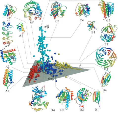
Proteins within each SCOP class are classified hierarchically at three additional levels: fold, superfamily, and family. In Figure 2.5, we show a visualization developed by the Berkeley Structural Genomics Center http://www.nigms.nih.gov/psi/image gallery/structures.html in which globally similar structures are grouped together and globally dissimilar structures are located far away from each other. This figure shows segregation between four elongated regions corresponding to the four SCOP protein classes: α, β, α/β, and α +β. Further details about protein structure classification can be found in [MBHC95].

Figure 2.5: The top level structural classification of proteins based on their secondary struc-ture components.

2.2 Protein Function

(35)

chemical reaction. Protein function can also be described at a physiological level concerning the whole organism, e.g. the impact of a protein on the functioning of an organism. We describe protein function at 3 different levels according to [OJT03]:

• Molecular function: A protein’s molecular function is its catalytic activity, its binding activity, its conformational changes, or its activity as a building block in a cell. [PR04].

• Cellular function A protein’s cellular function is the role that the protein performs as part of a biological pathway in a cell.

• Phenotypic function: A protein’s phenotypic function determines the physiological and behavioral properties of an organism.

We need to keep in mind that protein function is context-sensitive with respect to many factors other than its sequence and structure. These factors include (but are not limited to) the cellular environment in which a protein is located, the post-translation modification(s) of the protein, and the presence or absence of certain ligand(s). Though often not mentioned explicitly, these factors are important for protein function.

In this chapter, we concentrate on the molecular function of a protein. We do so since (1) it is generally believed that native structure may most directly be related to the molecular func-tion [GSB+05], (2) determining the molecular function is the first step in the determination of the cellular and phenotypic function of a protein.

2.3 The Importance of Local Structure Comparison

Traditionally global structure comparison is well investigated in protein structure analysis. Recently the research focus has shifted towards local structure comparison. The transition from global structure comparison to local structure comparison is well supported by a wide range of experimental evidence.

2.3.1 Protein Function

(36)

Biology has accumulated a long list of sites that have functional or structural significance. Such sites can be divided into the following three categories:

• catalytic sites of enzymes • the binding sites of ligands • the folding nuclei of proteins

Local structure similarity among proteins can implicate structurally conserved amino acid residues that may carry functional or structural significance [CLA99, WBL+_{03, DBSS00,}

KWK04].

Similar Structures, Different Function

It is well known that the TIM barrels are a large group of proteins with a remarkably sim-ilar fold, yet widely varying catalytic function [NOT02]. A striking result was reported in [NKGP90] showing that even combined with sequence conservation, global structure con-servation may still not be sufficient to produce functional concon-servation. In this study, Neidhart et al.first demonstrated an example where two enzymes (mandelate racemase and muconate lactonizing enzyme) catalyze different reactions, yet the structure and sequence identities are sufficiently high that they are very likely to have evolved from a common ancestor. Similar cases have been reviewed in [GB01].

Different Structures, Same Function

It has been also noticed that similar function does not require similar structure. For example, the most versatile enzymes, hydro-lyases and the O-glycosyl glucosidases, are associated with 7 folds [HG99].

In a systematic study using the structure database SCOP and the functional database Enzyme Commission (EC), George et al. estimated 69% of protein function (at EC sub-subclass level) is indeed carried by proteins in multiple protein superfamilies [GST+04].

(37)

Chapter 3 A Taxonomy of Local Structure

Comparison Algorithms

3.1 Introduction

As discussed in Chapter 1, a structure pattern is a geometric arrangement of elements, usu-ally at the amino acid residue level. Some other terminology also used for structure patterns includes structure templates [TBPT05] and structure motifs [EJT04]. All algorithms that identify structure patterns are generally known as the local structure comparison algorithms. Below, we introduce the common tasks in local structure comparison, the related computa-tional components, and typical algorithms for local structure comparison.

3.1.1 Tasks in Local Structure Comparison

The task of local structure comparison is to recognize structure patterns in proteins where the patterns may be known a priori or not. When patterns are known, the recognition problem is apattern matching problem in which we determine whether a pattern appears in a protein. When patterns are unknown, the recognition problem is apattern discovery problem in which we find structure patterns that appear in all or many of the protein structures in a group.

The pattern discovery problem can be subdivided into two groups. The first group is sequence-dependent pattern discovery that discovers structure patterns in which elements have conserved sequence orders. The second is sequence-independent pattern discovery that discovers structure patterns without considering the primary sequence order.

(38)

Pattern Discovery Pattern Matching

Protein Local Structural Comparison problem

Sequence-independent Sequence-dependent

Pair-wise comparison n-way comparison (n >>3)

ASSAM, Artymiuk et al., JMB’94

TESS, Wallace et al., Prot. Sci. ‘97

PINTS, Russell, JMB’98

TRILOGY,

Bradley et al., RECOMB’01

FFSM & its descendants,

Huan et al. ICDM’03, RECOMB’04

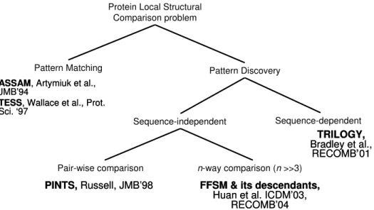
Pattern Discovery Pattern Matching

Protein Local Structural Comparison problem

Sequence-independent Sequence-dependent

Pair-wise comparison n-way comparison (n >>3)

ASSAM, Artymiuk et al., JMB’94

TESS, Wallace et al., Prot. Sci. ‘97

PINTS, Russell, JMB’98

TRILOGY,

Bradley et al., RECOMB’01

FFSM & its descendants,

Huan et al. ICDM’03, RECOMB’04

Figure 3.1: A taxonomy of local structure comparison algorithms.

3.1.2 Components

We list a group of three computational components: pattern definition, scoring function, and search procedure in order to complete the computational tasks outlined in the previous section. A pattern definition specifies the mathematical presentation of structure patterns, a scoring function measures the fitness of a pattern to a structure, a search procedure searches through a solution space and identifies the best solution(s) according to a pattern definition and a scoring function. Below we provide further detail of the three computational components.

Pattern Definition

A structure pattern is a geometric arrangement of structure elements, e.g. amino acids, in proteins. To provide the precise definition of structure pattern, we need to choose the elements in such definition. The typical choices are:

• atoms,

• amino acid residues,

• secondary structure elements (SSE)

(39)

computation than a coarse representation such as SSE. On the other hand, by choosing SSEs, we may miss valuable information about a protein structure. Early structure comparison used SSE extensively, mainly for the purpose of efficient computation. Recent research tends to use amino acid or atoms because of the detailed representation.

Once we choose structure elements, there are three widely used methods to define a structure pattern.

• Graph: A node represents a structure element in the structure. An edge represents the geometry of the protein, usually in terms of pair wise element distance.

• Point set: Each point represents a structure element in the structure, with the coordi-nates of the element.

• Point list: the same as point set but elements are ordered as their position in the primary sequence of the protein.

Scoring Function

A scoring function quantifies the fitness of a structure pattern to a structure. Choosing the right scoring function plays a central role in structure comparison and involves careful design. Two types of scoring functions are commonly used. First, subgraph matching determines whether a pattern (specified by a graph) matches a structure (specified by another graph) [Ull76].

Second, the least-square fit with rigid body transformation measures the closeness of a pattern (a point set) to a structure (another point set) [EJT04]. In least-square fit, we superimpose the pattern onto the structure such that the sum of the squared distances between corresponding elements is minimized [Kab78, Hor87]. The result of the least-square fit is conveniently expressed by a single value called the root-mean-squared-deviation (RMSD) between the pattern and the structure.

In parallel to the two methods listed previously, in matching a structure pattern with a protein structure, we may require that the structure elements in the pattern are totally ordered and the ordering is consistent with the primary sequence order of the matched ele-ments in the protein. If we enforce this sequence order requirement, we carry out a sequence dependent structure comparison, otherwise, we carry out a sequence independent structure comparison.

(40)

Search Procedures

Given the definition of structure patterns and a scoring function, asearch procedure is utilized to search trough a solution space and identify the best solution (s) according to the scoring function. Computational efficiency is the major concern for designing a search procedure. There are three types of commonly used search procedures:

• Subgraph matching determines whether a subgraph occurs in a graph. • Geometric hashing determines whether a point subset occurs in a point set.

• Frequent subgraph mining determines the group of recurring subgraphs in a collection of graphs.

The details of these search algorithms will be introduced in the following a few sections.

3.2 Pattern Matching

In pattern matching, we want to determine whether a pattern occur in a protein structure. Further more, if a pattern does occur in a protein structure, where it occurs and how many times it occurs in a protein structure. Typically, there are three types of subproblems in pattern matching [EJT04] as discussed below:

• Occurrencepattern matching determines whether a pattern occurs in a protein structure • Complete pattern matching finds all occurrences of a pattern in a protein structure • Probabilistic pattern matching calculates the probability that a pattern appears in a

protein structure.

The solution of the complete pattern matching problem can be used to answer the oc-currence pattern matching problem, but sometimes the latter can be computed directly in a efficient way. In the following discussion, we focus on complete pattern matching and present two algorithms: one based on subgraph isomorphism and the other one based on geometric hashing. For probabilistic pattern matching, see [AG04].

3.2.1 ASSAM

(41)

Pattern Definition

ASSAM uses a graph to represent a structure pattern where

• A node in the ASSAM graph represents an amino acid residue and is labeled by the identity of the residue.

• Every pair of nodes is connected by an edge. The edge is labeled by a distance vector (to be defined) between the two residues.

In ASSAM, an amino acid residue is represented as a two-element tuple (p1, p2) where

p1 and p2 are two points in a 3D space. These two points are selected to specify the spatial

location and the side chain orientation of the residue and are called the “pseudo atoms” in ASSAM 1_{. One of the two pseudo atoms in a residue} _R _{is designated as the “start” atom,}

denoted byS(R), and the other is the “end” atom, denoted byE(R). Refer to [APG+94] for how to obtain the pseudo atoms for the 20 different amino acids.

Thedistance vector VR,R0 between two amino acid residuesRandR0 is a sequence of four distances

VR,R0 =d(S(R), S(R0)), d(S(R), E(R0)), d(E(R), S(R0)), d(E(R), E(R0))

whered(x, y) is the Euclidian distance of two pointsx and y. The distance vector is used as an edge label in the graph.

ASSAM represents structure patterns in the same way that it represents full protein structures.

Graph Matching

A distance vector VR1,R2 matches another distance vector VR0₁,R0₂ if:

|d(S(R1), S(R2))−d(S(R01)), S(R02))| ≤ dss

|d(S(R1), E(R2))−d(S(R01)), E(R02))| ≤ dse

|d(E(R1), S(R2))−d(E(R01)), S(R02))| ≤ des

|d(E(R1), E(R2))−d(E(R01)), E(R02))| ≤ dee

where dss, dse, des, dee are bounds on the allowed variation in distances. These inequalities

help make the matching robust against structure uncertainty in structure determination. A structure patternU matchesa protein structureV, if there exists a 1-1 mapping between vertices inU and a subset of vertices in V that preserves node labels and edge labels.

(42)

ASSAM adapts Ullman’s backtracking algorithm [Ull76] to solve the pattern matching problem. We discuss the details of Ullman’s algorithm for subgraph matching in Section 4.3

3.2.2 TESS

TESS models both protein structures and structure patterns as point sets where each point represent an atom in the protein structure or structure pattern. TESS determines whether a pattern matches a structure using geometric hashing [WBT97]. Specifically, the matching is done in two steps. In the preprocessing step, TESS builds hash tables to encode the geometry of the protein structure and the structure pattern. In the pattern matching step, TESS compares the contents of the hash tables and decides whether the structure pattern matches the protein structure. With minor modifications, TESS can be extended to compare a structure pattern with a group of structures. See [PA98] for other pattern matching algorithms that also use geometric hashing.

Below, we introduce the detail of the TESS algorithm.

Pattern Definition

TESS represents a structure pattern as a set of atoms P = {a1, . . . , an} where n is the size

ofP. Each atom is represented by a two-element tupleai = (pi, idi) wherepi is a vector in a

3D space andidi is a nominal scalar that represents the identity of the atom.

Preprocessing in TESS

To encode the geometry of a protein structure, TESS selects three atoms from each amino acid residue and builds a 3D Cartesian coordinate system for the selection. Such 3D Cartesian coordinate system is also called a reference frame in TESS. For each reference frame, the associated amino acid residue is itsbase and the three selected atoms are the reference atoms of the frame. Predefined reference atoms exist for all 20 amino acid types [WBT97].

Given three reference atomsp1, p2, p3 where each atom is treated as a point, TESS builds

a reference frameOxyz in the following way:

• the origin of theOxyz system is the midpoint of the vector −−→p1p2,

• the vector −−→p1p2 defines the positive direction of the x-axis,

• pointp3 lies in the xy plane and has positive y coordinate.

• the positive direction ofz-axis follows the right-hand rule.

(43)

discretized into an index that is hashed into a hash table. The associated value of an index is a two-element tuple (r, a) wherer is the identifier of the base of the reference frame anda

is the identifier of the corresponding atom.

TESS builds a reference frame for each amino acid residue in a protein structure and hash every atom in the protein structure into the hash table as described previously. For a protein with a total of R residues and N atoms, there are a total of R×N entries in the TESS hash table since each reference frame produces a total ofN entries and there are a total of R

frames.

TESS performs the same preprocessing step for a structure pattern.

Pattern Matching

For a pair of reference frames, one from a protein structure and the other one from a structure pattern, TESS determines whether there is a hit between the protein structure and the structure pattern. A hit occurs when each atom in the structure pattern has at least one corresponding atom in the protein structure. TESS outputs all pairs of reference frames where a hit occurs.

TESS has been successfully applied to recognize several structure patterns, including the Ser-His-Asp triad, the active center of nitrogenase, and the active center of ribonucleases, in order to predict the function of several proteins [WBT97].

3.3 Sequence-Dependent Pattern Discovery

Discovering common structure patterns from a group of proteins is more challenging than matching a known pattern with a structure. Here we introduce two algorithms: TRILOGY [BKB02] and SPratt [JET99, JECT02] that take advantage of sequence order (and separation) information of amino acid residues in a protein structure to speed up pattern discovery. Patterns identified by these methods are sequence-dependent structure patterns.2

3.3.1 TRILOGY

TRILOGY identifies sequence-dependent structure patterns in a group of protein structures [BKB02]. There are two phases in TRILOGY: initial pattern discovery and pattern growth. Before we discuss the two phases in detail, we present the pattern definition and matching condition used in TRILOGY.

(44)

Pattern Definition

In TRILOGY, a three-residue pattern (a triplet)P is a sequence of amino acid residues and their primary sequence separations such that

P =R1d1R2d2R3

whereRi (i∈[1,3]) is a list of three amino acid residues sorted according to primary sequence

order in a protein and di (i∈ [1,2]) is the number of residues located between Ri and Ri+1

along the primary sequence (the sequence separation).

Each residue R in TRILOGY is abstracted by a three-element tuple (p, v, id) where p is a vector specifying the 3D coordinates of theCα atom in R, v is the vector ofCαCβ atoms,

andid is the identity of the residue.

Pattern Matching

A tripletP =R1d1R2d2R3matches a protein structure if there exists a tripletP0 =R01d01R02d02R03

in the structure such that

• (1) the corresponding amino acid residues (Ri and R0i, i ∈ [1,3]) have similar amino

acid types,

• (2) the maximal difference between the corresponding sequence separations |di −d0i|

i∈[1,2] is no more than a specified upper-bound (e.g. 5), • (3) the geometry of two triplets matches. This suggests that:

– the difference between the related Cα-Cα distances is within 1.5 ˚A

– the angle difference between two pairs of matchingCα-Cβ vectors is always within

60◦

If a protein satisfies condition (1) and (2) but not necessarily (3) it is asequence matchof the triplet P. If a protein satisfies condition (3) but not necessarily (1) or (2) it is a geometric match of the triplet P. By definition, a protein matches a triplet P if there is a sequence matchand a geometric match to P.

The pattern definition and matching condition for larger patterns withd amino acids are defined similarly to the above, but use 2d−1 element tuples instead of triples.

Triplet Discovery

(45)

After sequence alignment, all possible triplets are discovered. For each triplet, TRILOGY collects two pieces of information: the total number of sequence matches and the total num-ber of structure matches, and assigns a score to the triplet according to a hypergeometric distribution. Only highly scored triplets are used to generate longer patterns.

Pattern Growth

If a highly scored triplet shares two residues with another triplet, the two patterns are “glued” together to generate a larger pattern with four amino acid residues in the format ofRidiR4

where{Ri}, i∈[1,4] anddi, i∈[1,3] are defined similarly to ones in triplets. Longer patterns

in TRILOGY are generated similarly.

3.3.2 SPratt

Like TRILOGY, the SPratt algorithm also uses the primary sequence order information to detect common structure patterns in a group of protein structures [JET99, JECT02]. Un-like TRILOGY, SPratt discards the requirement that the sequence separation between two residues should be conserved. In the following discussion, we present the details of the SPratt algorithm.

Pattern Definition

In SPratt, a patternP is a list of amino acid residues

P =p1, . . . , pn

wherenis the length ofP. Each residue in SPratt is abstracted as a two-element tuple (p, id) where p is a vector representing the coordinates of the Cα atom in R and id is the identity

of the residue. Additional information such as the secondary structure information and the solvent accessible area may be included to describe a residue.

Pattern Matching

A pattern P of length n matches with a protein structure Q if we can find a sequence of amino acid residuesS =s1, . . . , sn sorted according to the primary sequence order inQsuch

that

• the residue identity ofsi matches with the residue identify of pi,i∈[1, n].

• the root-mean-squared-deviation (RMSD) value of the corresponding locations inP and

(46)

Pattern Discovery

Pattern discovery in SPratt is done in three steps. First, SPratt picks an amino acid residue and selects all neighboring residues within a cutoff distance. It converts the set of neighboring amino acid residues into two strings, called neighbor strings: one that includes all residues that precede the target residue in the sequence and the second that includes all residues that follow. Both strings are sorted according to the primary sequence order. For each amino acid residue and each protein structure in a data set, SPratt computes the neighbor strings and puts all the strings together. Encoding neighboring residues in this way, the neighbor strings reflect the primary sequence order but not the separation between any residues.

Second, the Pratt string matching algorithm [Jon97] is used to identify all sequence motifs that occur in a significant part of the data set.

Third, for each sequence motif, the geometric conservation of the motifs (measured by the pairwise RMSD distance between all the instances of the sequence motif) is evaluated. SPratt selects only those with significant geometric conservation.

3.4 Pairwise Sequence-Independent Pattern Discovery

In the previous section, we discussed algorithms that identify sequence-dependent structure patterns. In this section and the one that follows, we discuss algorithms that identify structure patterns without the constraint of sequence order, orsequence-independent structure patterns. We divide sequence-independent structure pattern discovery algorithms into two groups according to whether they work on a pair of structures or on an arbitrary collection of struc-tures. In this section, we review pairwise sequence-independent pattern discovery methods and in the next section we show how pairwise comparison can be extended to multiway comparison of protein structures. Pairwise sequence-independent pattern discovery methods include:

• Geometric hashing methods that represent protein structures as point sets and use geometric matching to find structure patterns [NW91, FWLN94].

• Graph matching methods that model protein structures as labeled graphs and perform subgraph matching to detect conserved patterns [GARW93, MSO03, SSR04, SAW03, WTR+03].

3.4.1 Geometric Hashing

(47)

of pattern matching as exemplified by the TESS algorithm in Section 3.2.2. Rather than repeating the discussion of preprocessing and geometric matching that are common to almost all geometric hashing based methods, we present an analysis of computational complexity. We also show how different techniques may reduce the asymptotic complexity of the computation.

Pattern Definition

A structure is represented as a set of amino acid residuesP ={a1, . . . , an}wherenis the size

ofP. Each residue is represented by a two-element tupleai= (pi, idi) wherepi is a vector in

a 3D space that represents the spatial location of the residue (e.g. the coordinates of theCα

atom) and idi is the identity of the residue.

This definition was originally used by Nussinov & Wolfson [NW91]. The complexity of preprocessing a single protein structure withnresidues is bounded byO(n4). This is because there are a total of n₃

triplets in a protein. For each triplet we build one reference frame. For each reference frame, we compute the new coordinates of all n residues in the protein according to the frame. The complexity of this preprocessing step is hencen·O( n₃

) =O(n4_).

At the matching stage, two structures are preprocessed and the results are stored in a single hash table. After preprocessing, we scan the hash table once to report the shared structure patterns. Clearly, the post processing step is bounded by the total number of entries in the hash table which is itself bounded byO(n4). Therefore the overall computational complexity isO(n4_).

Nussinov & Wolfson present an algorithm to speed up the computation from O(n4_{) to}

O(n3). In the improved version, rather than using a triplet to build a reference framework, two points are used to build a reference framework. There are a total ofO(n2_{) point pairs in}

a data set withn points and hence the overall complexity is reduced toO(n3).

Fischer et al.[FWLN94] proposed a more efficient algorithm with complexity O(n2). For a protein structure with n residues, rather than building a total of O(n3_{) reference frames,}

Fischer’s method builds a total ofnreference frames. This is done by always picking up three residues that are consecutive in the primary sequence and building one reference frame for each such triplet. There are a total ofO(n) such triplets so the overall complexity isO(n2_).

Geometric hashing has been applied to recognize local structure similarity for proteins even if they have globally different structures [FWLN94].

3.4.2 PINTS