SELF-ORGANIZATION OF THE CLIMATE SYSTEM: SYNCHRONIZED POLAR AND OCEANIC TELECONNECTIONS
Elizabeth Piccard Reischmann
A dissertation submitted to the faculty of the University of North Carolina at Chapel Hill in partial fulfillment of the requirements for the degree of Doctor of Philosophy in
the Department of Geological Sciences.
Chapel Hill
2016
Approved by: José A. Rial Jonathan M. Lees
ii © 2016
iii ABSTRACT
Elizabeth Piccard Reischmann: Self organization of nonlinear Paleoclimate and climate oscillators
(Under the direction of José A. Rial)
iv
v
vi
ACKNOWLEDGMENTS
vii
TABLE OF CONTENTS
LIST OF TABLES………….………..…...ix
LIST OF FIGURES………..………...x
CHAPTER 1: AN INTRODUCTION TO SYNCHRONIZATION IN THE CLIMATE SYSTEM…....………...………..………...1
1.1.Introduction………...….1
1.2. Amplitude Modulation of the Global Climate System………..3
1.3.Synchronization of the Polar Climates Over the Last Ice Age ………...17
1.4.Supplemental Materials………39
1.5.References……….…………...53
CHAPTER 2: DETECTING THE THERMOHALINE CIRCULATION’S PERIODICITY: HOW POLAR PALEOCLIMATES COMMUNICATE...59
2.1. Introduction………..………..……….59
2.2. Supplemental Materials………..71
2.3 References………….………77
CHAPTER 3: SYNCHRONIZATED DIPOLE-LIKE SEA SURFACE TEMPERATURE OSCILLATIONS IN THE SOUTHERN HEMISPHERE……….……….….…… 80
3.1. Introduction………..……….…..………80
3.2. Supplemental Materials……..………..…….………..95
3.3. References………...…….….111
CHAPTER 4: IN SEARCH OF INTERMEDIATE, INTER-PROXY COMPARISONS: A NOTE ON COMPLEXITIES OF AGE MODELS………....….……115
viii
4.2 References………..………129
APPENDIX 1: CHAPTER ONE SUPPLEMENTAL INFORMATION………..132
S1.1 Frequency Modulation…………...………132
S1.2 Nonlinear Synchronization………...……….135
S1.3 Effect of Amplitude Modulation………..……….137
S1.4 Effect of Noise………..……….137
APPENDIX 2: CHAPTER TWO SUPPLEMENTAL INFORMATION………...139
S2.1 Age Model Details and Reasoning………...………..139
S2.2 Methods and Materials………...………140
APPENDIX 3: CHAPTER THREE SUPPLEMENTAL INFORMATION.………..142
S3.1 Supplemental Discussion of ENSO and ACW………..………142
ix
LIST OF TABLES
x
LIST OF FIGURES
Figure 1.1 Frequency modulation of LR04………...………...5
Figure 1.2 The modulator and eccentricity..………..……….………...6
Figure 1.3 Frequency bands of synchronization………...8
Figure 1.4 Spectral power transfer………..……...……….……...9
Figure 1.5 Age model matching………...…..………...20
Figure 1.6 Phase relationship………..……….22
Figure 1.7 Stability of phase relationship………...……….……23
Figure 1.8 Filtering methods robustness………...……….…….……….26
Figure 1.9 Simulation results and data comparison………..……...…29
Figure 1.10 Forcing robustness and effects……….……….………..………...…31
Figure 1.11 Model stability to changes in forcing………...……….………….33
Figure S1.1 Data and Fm(t) comparison………...……....….39
Figure S1.2 Data spectra………..………...……..….40
FigureS1.3 Model spectra………...……..….41
Figure S1.4 Forced and unforced spectra………...……..….42
Figure S1.5 Spectrogram of LR04 stack.………...……..….43
Figure S1.6 Phase relationship details………...………..….44
Figure S1.7 Phase relationship details………...……..….45
Figure S1.8 Phase relationship details ………...……….….46
Figure S1.9 Phase relationship evolution………...……..….47
Figure S1.10 Details of the power transfer of all power lobes………...……..….48
xi
Figure S1.12 Eccentricity forcing strength test………...……..….50
Figure S1.13 Tuned vs. unturned LR04 results…...………...……..….51
Figure S1.14 Phase relationship with and without amplitude modulations.…………...……..….52
Figure 2.1 Log-log deconvolution of 12 polar pairs………..62
Figure 2.2 Transfer function time series and spectra………..……...65
Figure S2.1 Linear deconvolution spectra………...……...71
Figure S2.2 Regularization parameter tests………...……...72
Figure S2.3 Linear and log deconvolution tests………...……...73
Figure S2.4 NGRIP and DomeC transfer function………...……...74
Figure S2.5 Model and data deconvolution comparison………...……...75
Figure S2.6 Model transfer function………...……...76
Figure 3.1Correlation coefficient map of dipoles and time series…………...………...………..87
Figure 3.2 Precipitation anomaly correlation map……….………91
Figure S3.1 EOF map for the dipoles………..….……...95
Figure S3.2 Correlations with 2nd reanalysis data set………..….……...96
Figure S3.3 Satellite era correlation………..….…..…...97
Figure S3.4 Monthly stack correlations for SPDO...………..….……..98
Figure S3.5 Monthly stack correlations for SIDO...………..….……..99
Figure S3.6 SPDO DMI vs SLPA and U-wind...………..….….……100
Figure S3.7 Monthly SPDO DMI vs SLPA...………..….…………...101
Figure S3.8 SIDO DMI vs SLPA and U-wind...………..….……...102
Figure S3.9 Monthly SIDO DMI vs SLPA...………..….………...…103
xii
Figure S3.11 2nd Precipitation data set analysis...………..….………105
Figure S3.12 AR1 model independence test...………..………..….………106
Figure S3.13 Dipole deconvolution and transfer functions...………..…..……..107
Figure S3.14 Dipole map………....………..….……..108
Figure S3.15 Dipole correlation maps...………..….………...109
Figure S3.16 Dipole time series…………...………..….…………..110
Figure 4.1 Indexed available sediment cores……….……….……122
Figure 4.2 Spatially distributed sediment cores against LR04 stack……….…………..…123
1
CHAPTER 1: AN INTRODUCTION TO SYNCHRONIZATION IN THE CLIMATE SYSTEM 1.1 Introduction
2
eccentricity (which modulates the amplitudes of the orbital 100-kyr eccentricity and precession) phase locked, frequency entrained, frequency modulated, and amplified [Pikovsky and Kurths, 2002; Rial, 2012] the free oscillations of the climate system during the past 1.2 Myr, the discovery of which was the basis of the work in this thesis. Prior to this work, the study of phase relationships in the climatic signals was performed on modern, directly observational signals. While some uncertainty is definitely present in the LR04 stack, tuned or un-tuned, for reasons thoroughly discussed in Chapter 4, on the scale of 100kyr periodicities, these uncertainties are not significant.
3
Part 1.2: Amplitude Modulation of the Global Climate System via the 413-kyr Orbital
Eccentricity Cycle.1
Since about 1.2-1.3 million years ago, glacial–interglacial cycles have had a period of about 100,000 years. Prior to this point, the cycles had lower amplitudes and an approximately 40,000 periodicity [Clark et al., 2006]. This shift does not correspond to a known change in the physical features of the globe, and is known as the mid-Pleistocene transition. Both of these cycles have nearly corresponding Milankovitch cycles, i.e., cycles of changes in orbital features. However, the magnitude of the change in incoming solar radiation due to the 100kyr cycle— insolation—at this timescale is small, and therefore difficult to reconcile with the amplitude of the glacial cycles [Lisiecki, 2010; El-Kibbi and Rial, 2001; Huybers and Wunsch, 2005; Raymo, 1997; Berger et al., 2005; Clark et al., 2006]. As mentioned above, our group has focused on synchronization as a climate organizing mechanism. Using spectral analyses aided by a numerical model, we found that the climate system signal as recorded in the LR04 prxy stack synchronized to the 413,000-year eccentricity cycle about 1.2 million years ago and has remained synchronized ever since. This synchronization allows for a nonlinear transfer of power and frequency modulation that increases the amplitude of the 100,000-year cycle. We conclude that the forced synchronization can explain the strong 100,000-year glacial cycles through the alignment of insolation changes and internal climate oscillations.
The search for synchronization in this dataset was motivated by previous work done by Rial [1999] which noted that untuned climate proxy records show a frequency [Van der Pol,
_________________________________________
4
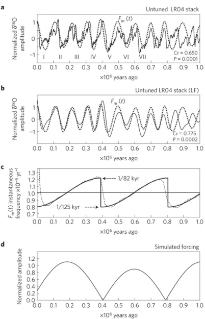
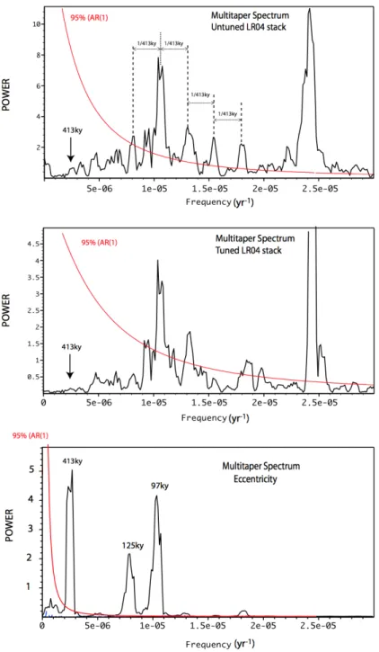
1930; Lathi and Ding, 2009]. The LR04 time series specifically shows that the 100kyr glacial cycles are modulated by a 413kyr cycle, i.e. orbital eccentricity (Fig. 1). In the frequency domain, multi-taper [Ghil et al., 2002] spectra of both the untuned LR04 data and Fm(t) (a simple model approximating the LR04 stack, see Methods) also have the side-lobe frequencies 1/125, 1/77, 1/64 and 1/55 kyr. These side lobes are spaced around the ~ 1/100-kyr peak at spectral distances equal to integer multiples of 1/413 kyr, once again indicating that this is our modulating signal [Rial, 1999; Van der Pol, 1930,; Lathi and Ding, 2009].
5
6
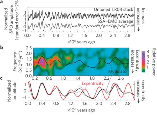
Frequency modulation in the paleoclimate also implies the existence of a modulator, which is also known as the intelligence of the modulated system. This intelligence, calculated via the Gabor method of taking the envelope of the rectified time dericatived of the low-pass filtered 5-million-year-long LR04 stack, should represent a proxy for the climate’s response to forcing (shown in Figure 2, details of the calculation in Methods [Lathi and Ding, 2009] from a modulated time series.
7
is the mean and dashed lines are ±1σ . The modulator function represents the forcing as seen from the climate system’s reference frame. All calculations are performed using the complete 5-Myr record.
8
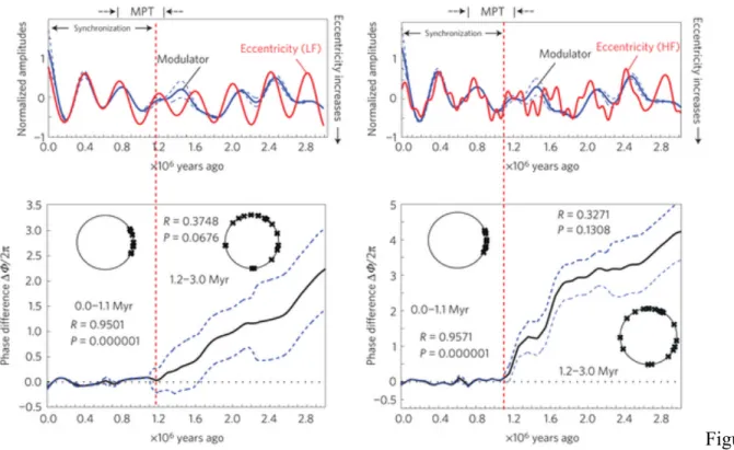
Figure 1.3. Theoretical low-frequency (period > 300 kyr) and high-frequency (period > 80 kyr) orbital eccentricity compared with the modulator (top). Their phase difference (see Methods) decreases monotonically (bottom) with time until phase locking occurs about 1.2–1.1 Myr ago. Mean value (solid) ±1σ (dashed) of are shown. In the insets it is shown that the Rayleigh R test and P values (see Methods) reject the null hypothesis of phase circular uniformity in the 1.2–0 Myr ago interval, so that the abrupt change in Φ(t) at ∼1.2 Myr ago is statistically significant. The LR04 time series and the 100-kyr eccentricity have previously been shown to be phase locked in the 1.2–0 Myr ago interval using a wavelet approach.
9
were increasing or decreasing, resulting in frequency-modulated internal ~ 100-kyr cycles reaching unprecedented amplitudes during the late Pleistocene.
10
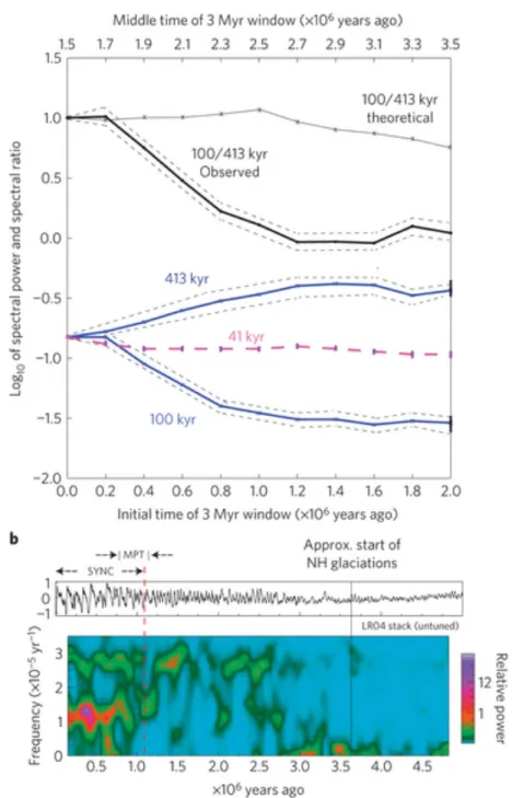
estimates of spectra measurement error. b, Spectrogram showing the time evolution of the power in the 1/41-, 1/100- and the 1/413-kyr frequency bands. The higher resolution shows details missed by the long-term trends in a.
One other event that strongly suggests energy transfer across frequencies is the relatively brief period of nonlinear resonance that, as suggested by Fig. 2c, happened when ΔΦ(t)≈0 and frequency detuning ΔΩ≈0 occurred simultaneously about 400 kyr ago (see Methods). That is, the time when the spectrogram in Fig. 2b records the largest power in the signal lasting not longer than ~ 20 kyr. The warming trend of low eccentricity reinforced by internal feedbacks working in unison with the forcing rapidly shrunk the ice sheets, resulting in the high-frequency (~ 1/82 kyr) unusually warm interglacial episode at marine isotope stage 11 (MIS11; Fig. 2). We can infer that the amplitude of the response became strong enough to nonlinearly shift the system away from resonance, which explains the brevity of the resonant interval. Similar astronomical circumstances (low eccentricity) also occurred at ~ 0.8 Myr ago and are happening today, but both then and now, as seen in Figs 2c and 3, the instantaneous frequencies are distinct (within time uncertainty), and .
11
In contrast, the spectral power in the 1/41-kyr (obliquity) band increased slowly from 5 Myr ago, reached a maximum around 1.2 Myr ago and then remained nearly constant [Lisieki and Raymo, 2007] until the present time. It has been suggested that the 41-kyr obliquity forcing paces the glacial terminations [Huybers and Wunsch, 2005], but neither the simple function
Fm(t) (Fig. 1 and Supplementary Fig. S1) nor the nonlinear ice volume model (Supplementary Fig. S4) required 41-kyr obliquity forcing which, accordingly, does not seem necessary to account for the timing of the glacial terminations. Further, frequency modulation does not require the climate state to arbitrarily select skipping one rather than two obliquity beats before deglaciation takes place [Huybers and Wunsch, 2005], while forced synchronization explains the MPT without further assumptions.
12
There is also suggestive evidence for synchronization in the time evolution of the modulator’s instantaneous phase ΦC: Supplementary Fig. S9 shows that the phase of the modulator, basically constant before 4 Myr ago, begins to approach the phase ΦF of the eccentricity forcing around the start of the Northern Hemisphere Plio–Pleistocene glaciations at ~ 3.6 Myr ago [Lisiecki and Raymo, 2007]. From this time on, the eccentricity forcing seems to drive the climatic response, because the modulator’s phase approaches the eccentricity’s phase in a nearly smooth and apparently deterministic fashion until both synchronize around 1.2–1.1 Myr ago and both share the same frequency (1/413 kyr). In fact, the instantaneous frequency of the modulator (given approximately [Gabor, 1946] by the time-averaged slope of ΦC) increases from ~ 0 at 5 Myr ago to ~ 1/413 kyr at 1.2 Myr ago. Consistent with these observations, the modulator is of low frequency and low amplitude before the start of the Northern Hemisphere glaciations (see Supplementary Fig. S10).
13
power (Fig. 4), which results in an increased bandwidth of the ~ 100-kyr glacial cycles due to frequency modulation (Supplementary Figs S2 and S4).
Synchronization allowed energy from the sun to flow into or out of the climate system at the same time internal feedbacks were warming or cooling it, resulting in unprecedentedly large climate fluctuations that powered the great Pleistocene glaciations (a process akin to resonance of a forced linear oscillator). Forced phase synchronization, which is still occurring, started 1.2 Myr ago, and culminated at the time of the MIS11 (~ 0.4 Myr) with a brief period of nonlinear resonance. During synchronization, the 1/413-kyr component of eccentricity forced the frequency modulation of the ~ 1/100-kyr band, evidenced by depleted spectral power at 1/413 kyr and the presence of power at frequencies absent in the spectrum of the orbital forcing. Today resonance has faded but frequency modulation persists, driving the ~ 1/82–1/125-kyr frequency deviation that paces the timing of the major glacial terminations [Raymo, 1997].
Methods:
Master–slave synchronization.
The condition for (phase) synchronization can be expressed as
14
simultaneously with ΔΦ(t) = 0 around the MIS11 time (Fig. 2c), an event described here as nonlinear resonance. The time series in Figs 2 and 3 show that the instantaneous phase and its derivative (instantaneous frequency) are nearly the same at 400 kyr ago, even allowing for age uncertainty, so it is not improbable that they are resonating. The instantaneous phase is computed using the standard analytic function procedure [Gabor, 1946]. The brackets denote a time average so that ΔΩ is the difference in mean frequencies [Balanov et al., 2009].
Frequency modulation.
Clear evidence of frequency modulation is usually difficult to demonstrate unless the proxy records are astronomically untuned8. Tuning to the astronomical clock destroys frequency or phase modulation information (see Supplementary Fig. S2) and implies unwarranted [El-Kibbi and Rial, 2001; Clark et al., 2006; Saltzman, 2002; Rial, 1999; Pisias and Moore, 1981; Paillard, 1998; Muller and McDonald, 2000; Tziperman et al., 2006] linear relationships (proportionate amplitudes frequencies and phases) between external forcing and response.
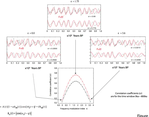
The signal Fm(t) introduced in Fig. 1 (see also Supplementary Fig. S1) is
15
eccentricity waveform the modulating frequency is ωm/2π = 1/826 kyr, so that the rectified cosine hm(t) has the correct 1/413-kyr frequency of the eccentricity cycle. The phase ψ is set equal to the actual value (Fig. 1d). ωc/2π is a natural oscillation frequency (carrier) of the climate system, assumed to be ~ 1/100 kyr. A(t) is a slowly varying negative linear ramp constructed ad hoc to attenuate the signal for early times. The frequency modulation index, ε = Δωc/ωm, is the ratio of the mean frequency deviation of the carrier (1/82–1/125)/2 to the
modulating frequency (1/826) [Rial 1999; Lathi and Ding, 2009]. For a rectified cosine of frequency 1/826 kyr the modulation index ε should be ~ 1.73, close to the calculated value ε = 1.75 that produces the highest correlation coefficient (0.775) between Fm(t) and the filtered LR04 stack over the past 0.8 Myr. The amplitude modulation index a = 0.25 is consistent with weak amplitude modulation. Besides a, the constant phase ϕ is the only other adjustable parameter in equation (1).
Extracting the modulator from LR04 stack.
16
17
Part 1.2: Synchronization of the Polar Climates Over the Last Ice Age2
1. Introduction
Having established the roll of forced synchronization in the Mid Pleistocene Transition, we now turn our focus to the synchronization of the ice sheets. The climate records seen in the polar ice cores can also be characterized as nonlinear, complex, oscillating systems, with periods of abrupt warming separated by abrupt cooling. Here, we demonstrate the effectiveness of modeling the polar climates as synchronized, nonlinear oscillators, using the same ice volume model (Saltzman, 2002) used in the previous section, only here we use two coupled systems, each of which represents one polar climate as simple Van der Pol oscillators.
Research identifying and modeling the polar climates’ similar dynamics can be summarized as follows: “The EPICA Community Members (2006) identified a linear relationship between the stadial intervals at the poles during the MIS3 interval 50 ka–30 ka (1 ka = 1000 years ago). Prior to this, Crowley had put forward the basic bipolar hemispheric seesaw hypothesis (Crowley, 1992; Broecker, 1998) as an explanation of how the abrupt warming episodes in the North Atlantic lead to the beginning of cooling episodes in Antarctica, namely via polar climate communication through meridional (equatorially asymmetric) heat transport and North Atlantic deep water (NADW) production. Blunier et al. (1998) and Blunier and Brook (2001) built on this idea, demonstrating that events in Greenland's climate follow those in Antarctica by about 1–3 ky (1 ky = 1000 years) and that this is due to the ocean controlling the climate at both poles. Hinnov et al. (2002) studied the specific connection between the Byrd and GISP2 records' inter-hemispheric anti-phasing (180° phase shift) of the
_________________________________________
18
Dansgaard–Oeschger (DO) oscillations over the 10–90 ka interval. Even more recently, Steig (2006) reported a π/2 phase shift between the polar climates, seen by analyzing high-resolution records from EDML (Antarctica) and NGRIP (Greenland) cores. Barker et al. (2009) then published data from the South Atlantic which demonstrated the existence of rapid but opposite temperature changes occurring at the same time as those documented in the north and proposed a link between the DO oscillations in the Arctic and the sub-Antarctic temperature variations. In a follow up study, they used Crowley's simple, conceptual bipolar seesaw model to forecast the unknown Greenland record using the 800 ky record of Antarctica (Barker et al., 2011), though the lack of actual Greenland records beyond ∼120 ka means that they were unable to validate their results. Finally, in response to this, Rial (2012) proposed the nonlinear phase synchronization of the millennial-scale polar climates fluctuations during the last glaciation as an explanation for the apparent teleconnection between the Polar Regions.”
19
To clarify, the term synchronization or phase synchronization refers to frequency entrainment and phase lock (i.e. a constant phase difference), and is not the opposite of
asynchronous as used by some authors to refer to the polar climate being locked out of phase
20 Fig. 1.5.
21 2. Polar synchronization paradigm
2.1. Polar synchronization
As mentioned earlier, in order for synchronization to be established, phase lock must be present between two or more, interacting time series. Note that the phase lock can either be in-phase, anti-in-phase, or an arbitrary, constant phase. For the polar regions, all millennial scale frequency components in the signal are π/2 phase locked, meaning each of a pole’s frequency components is shifted by one-fourth of its period to align with the other. Thus time series pairs like NGRIP-DomeC or GRIP-Byrd can be formally described as approximate Hilbert transform pairs (Bracewell, 1986; see Appendix A).
22 Fig. 1.6.
23
signal, a procedure equivalent to a Hilbert Huang Transform (HHT) (Huang et al., 1998). To obtain the phase shifted signal, we applied HHT (equivalent to a −π/2 shift) to the Dome C record with integral limits from past to future (see Appendix 1).
Fig. 1.7.
24 2.2. Transforming one polar climate into the other
The quantified phase difference calculations shown in Fig 1.5-7 require precise instantaneous phase calculations, which is a non-trivial process. To begin, as mentioned earlier, a set of relative dates are established via a pair of methane records from the two poles (e.g. Blunier et al., 1998; Capron et al., 2010). These chronologies were then extended via a Monte Carlo approach (e.g., adapted from Blunier et al., 2007). This gives us 7 cores and 12 pairs of records to work with.
In order to determine the instantaneous phase of these now comparable time series, analytical functions are constructed for each time series (see Appendix A) (Gabor, 1946). The ice core temperature proxy signals are complicated signals, whereas the Hilbert Transform is only proven accurate on components (Cohen, 1995; Huang et al., 1998). Therefore, the mono-components of the signal polar signals were extracted using the Empirical Mode Decomposition (EMD) (Huang et al., 1998) which provides Intrinsic Mode Functions (IMF). The HT is then applied to each mono-component signal (each IMF), a procedure equivalent to a Hilbert Huang Transform (HHT) (Huang et al., 1998). To obtain the phase shift transformed signal, we employed HHT (equivalent to a −π/2 shift) and inverse HHT (+π/2 shift) with integral limits from past to future (see Appendix A).
25
range. Our observations indicate that the phase shift is frequency independent, as all Fourier components are shifted by π/2, at least in the period band 1 ky–6 ky.
Figure 1.6 shows the full results of the comparison between NGRIP in the north and the HT of Dome C in the south. As shown in Fig. 1.7, the calculated phase lock is nearly constant and equal to π/2 modulo 2π. Sudden phase jumps of 2π, which occur during abupt de-synchronization episodes (Fig. 1.7), are likely excited by noise, timing errors or external forcing and do not persist for long periods.
3. Simulation of Antarctic climates from Greenland climates 3.1. Frequency band separation
In order to begin to build our model, we separate the polar signals into two bands, above and below 50 kyrs. The 800 kyr-long EPICA proxy records (and most temperature proxy records for the last million years) also have a well established tendency of consisting of easily identifiable and disjointed groups of statistically significant power peaks in the long period band (>70 kyr) and the short period band (<45 kyr), with little or no interaction between the two. The latter is assumed to reflect the high frequency response of sea ice, while the former reflects the long period response of the major ice sheets to eccentricity-induced changes in insolation.
26
time series (e.g., Gloersen and Huang, 2003; Lin and Wang, 2006; Sole et al., 2007; Huang and Wu, 2008) and are described in detail in Appendix D.
Fig. 1.8.
27
Dome C, shown in Fig. 1.8, shows very little distortion in either the long or the short band, suggesting a true separation of the processes that produced the long and short period signals in both a linear and nonlinear combination.
3.2. Modeling the climate of the South from that of the North
In climate science, there are few well-established, simplified models that include both aperiodic forcing and stochastic effects (as are needed for polar modeling), but many areas of science indicate that relaxation oscillators are excellent candidates for the simulation of natural nonlinear oscillators. The Van der Pol oscillator is one of the most common, and has already been applied in climate sciences. Saltzman and Moritz (1980), Saltzman et al. (1981), Saltzman and Sutera (1984) and later Saltzman (2002) formally introduced a set of nonlinear, ordinary differential equations for sea ice extent and average ocean temperature in a glacial atmosphere equivalent to a Van der Pol/Duffing oscillator, which have since been widely adapted (Yang and Neelin, 1993; Zhang et al., 1995; Egger, 1999; Rial and Yang, 2007; Stommel, 1961; Källén et al., 1979; Paillard, 1998; Schulz et al., 2004; Colin de Verdière et al., 2006; Marchal et al., 2007; Crucifix , 2011; Rial and Saha, 2011; Crucifix, 2012; De Saedeleer et al., 2013).
28
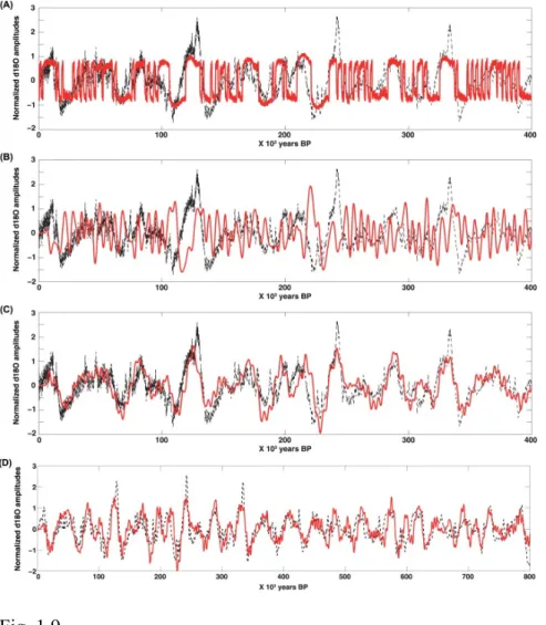
29 Fig. 1.9.
(A) The simulated record of Greenland temperature variation (red) and the high frequency (HF) component of the EPICA record. (B) The simulated Antarctic record without synchronization. (C) The Greenland record transformed by the VSO model into a synchronized Antarctica record compared to the actual time series (black). (D) The simulations (red) for the HF EPICA for the last 800 ky compared to the actual records (black). Parameter values for the results (D): q1 = 1000, q2 = 0, a1 = 0, a2 = 0.06, TN = 1500, TS = 2400, noise level = 0.55.
30
31 Fig. 1.10.
(A) Long period (∼100 ky) simulation using the ice sheet model without external forcing. Epica Dome C temperature proxy data (black) and simulated ∼100 ky components (red) are shown. (B) The model is externally forced by rectified cosine curve (blue line) that simulates the 413 ky eccentricity forcing. (C) The simulations (red) for the HF and low frequency components together for the last 800 ky compared to the actual records (black). Parameter values for the results (C) are same with those for Fig. 1.9D.
32
800 ky. Fig. 1.10C shows the long period component from the ice sheet model added to the simulated high frequency signal.
3.3. Model stability under parameter uncertainty
33
and where the parameter uncertainty is restricted to smaller than the uncertainty from the stochastic term.
Fig. 1.11.
Stability of the VSO model simulation as changing parameter values. (A) Correlation coefficient and RMSE as the forcing level a2 increases from 0 to 0.5. Strong external forcing makes the model to be controlled only by the forcing, so the model produces large errors for a2 > 0.1. (B) Correlation coefficient and RMSE as periods TN and TS range from 0 to 5000 years. When either TN or TS are less than 750 (white region), the model results diverge. The oscillation parameters bounded by the blue rectangular produce the smallest uncertainty (i.e. the stable regions for both TN and TS range from 750y to 4200y). (C) Correlation coefficient and RMSE as q1 increases from 0 to 1000 and q2 from 0 to 50. The VSO model produces stable simulations when q1 > 60.
34
VSO model parameter values which produces stable simulation of Antarctica temperature proxy for the last 800 ky.
Parameter Range Function
q1 60∼6000 Rate of mean ocean temperature change between Arctic and Antarctic
q2 0 Mean ocean temperature change between Arctic and Antarctic
a1 0 External forcing to north
a2 0.05∼0.12 External forcing to south TN 750∼4000 Oscillation (north) TS 750∼4000 Oscillation (south)
a1 and a2 adjust strength of external insolation forcing (a1: north, a2: south). These parameters modulate how strongly the insolation affects the natural oscillation of the climate. (a) The parameters are large enough: simulated results from the VSO model are completely dependent on the insolation. (b) These parameters are too small: the simulated results are independent of the insolation. Temperature fluctuation at millennial scale should be between (a) and (b). Though it is impossible to calculate the exact amount of insolation affecting the millennial scale climate oscillation, we suggest the range of parameter values that could produce compatible simulation with the observation.
35
Fig. 7 shows the model uncertainty from the parameters. The model behavior according to the parameter uncertainty and the ranges of the parameters that produce smaller effects than stochastic forcing can be summarized as follows:
i) Insolation parameters (a1, a2), Fig. 1.11A: Parameter ai regulates the strength of external forcing. The synchronization model originally included two forcing terms (a1, a2) at each pole (Eqs. (B.1) and (B.3)), but we use only one external forcing term (a2) in the south for this simulation. Strong external forcing overwhelms the model's responses to the other parameters (q and ω), thus a2 has to be constrained under a certain value because when external forcing is too strong, the simulated time series just follows the shape of forcing. From Fig. 1.11A, calculated as a2 increases, the model produces stable simulation when 0.05 < a2 < 0.10.
ii) Oscillation parameters (ω1, ω2), Fig. 1.11B: The angular frequencies ω1 and ω2 are given by ω1=2π/TN and ω2=2π/TS where TN and TS are the assumed periods of the natural oscillations of the North and South climates respectively.
The model produces close simulations when the periods are within both the millennial scale and the range of the assumed period of the thermohaline circulation (Marotzke et al., 1988; Bond et al., 2001). Fig. 1.11B shows the range of the natural frequency parameters which produces smaller uncertainty and a close simulation of Antarctic Records (e.g. TN: 1500yr and TS: 3000yr or vice versa).
36
cannot be used as a criterion for selecting best parameter values in this case. The results show that the correlation coefficients dramatically decrease as q2 increases and the model produces stable outputs when q1 > 60 and q2 < 10. Consequently, the reactive coupling term (q2) can be dropped in modeling while the dissipative term (q1) is required to be strong for both smaller uncertainty and a close simulation of the Antarctic temperature proxy.
4. Discussion
The results of both model and data study support a continuous phase synchronization of the polar climates for the length of the records. The physical processes behind this are not fully understood, but, as the next chapter demonstrates, evidence points to the thermohaline circulation as the most likely driver of the climate connection between the poles. The models we used to characterize the connection are robust with respect to changes in the adjustable parameters, and suggest that the connection between northern and southern climates is strongest when it involves the dissipative properties of the ocean/atmosphere, namely the difference between northern and southern heat flux.
37
polar climates were once unrelated to each other and likely chaotic, and that, through weak oceanic/atmospheric coupling, the two polar systems eventually synchronized by slowly modifying their own frequencies and phases to respond to each other's influence, until synchronization ensued and stabilized.
5. Conclusions
This study presents statistical investigations to explore and quantify the long-term relationship between Greenland and Antarctica's climate variability with polar synchronization as a mechanism to connect them, as well as presenting simplified, easily computable, and stable models for the last 800 ky of the polar paleoclimates. Using methane-matched records from GRIP and Byrd ice cores, we were able to match the age models of NGRIP and Dome C ice core records through a Monte-Carlo approach. Further, analysis of the model uncertainty with such minimal relative age uncertainty supports that simulated results are robust under small change of parameters. Use of this model and the simplified view of a highly complex system would be helped by further explanation of the underlying physical processes of the polar climates. However, synchronization as a paradigm for the linking of polar climate processes is well supported by our results and takes us a step further in our understanding of large-scale climate dynamics.
Part III: Conclusions
38
39
Supplemental Figures:
Section 1
40
41
42
Figure S4
43
Figure S5
44
Figures S6-S8
These figures (S6-S8) show details of the analysis summarized in Fig. 1.7.
47
Figure S9
48
Figure S10
Modulator, HF forcing, phase difference function ΔΦ(t) and spectrogram of the LR04 stack showing the time evolution of the power in the 1/41ky, 1/100ky and 1/400ky frequency
49
Figure S11
50
Figure S12
51
Figure S13
52
Figure S14
53 REFERENCES
Balanov, A., Janson, N., Postnov, D., Sosnovtseva, O., 2009. Synchronization, From Simple to Complex. Springer-Verlag, Berlin, Heidelberg, p. 425.
Barker, S., Diz, P., Vautravers, M.J., Pike, J., Knorr, G., Hall, I.R., Broecker, W.S., 2009. Interhemispheric Atlantic seesaw response during the last deglaciation. Nature 457, 1097e1102. Barker, S., Knorr, G., Edwards, L., Parrenin, F., Putnom, A.E., Skinner, L.C., Wolff, E., Ziegler, M., 2011. 800,000 Years of abrupt climate variability. Science 334, 347e 351.
Bennett, M., Schatz, M.F., Rockwood, H., Wiesenfeld, K., 2002. Huygens’ clocks. Proc. R. Soc. London A 458, 563e579.
Berger, A., Melice, J. L. & Loutre, M. F. On the origin of the 100-kyr cycles in the astronomical forcing. Paleoceanography 20, PA4019 (2005).
Blunier, T., Chappellaz, J., Schwander, J., Dallenbach, A., Stauffer, B., Stocker, T.F., Raynaud, D., Jouzel, J., Clausen, H.B., Hammer, C.U., Johnsen, S.J., 1998. Asyn- chrony of Antarctic and Greenland climate change during the last glacial period. Nature 394, 739e743.
Blunier, T., Brook, E.J., 2001. Timing of millennial-scale climate change in Antarctica and Greenland during the last glacial period. Science 291, 109e112.
Blunier, T., Spahni, R., Barnola, J.M., Loulergue, L., Schwander, J., 2007. Synchronization of ice core records via atmospheric gases. Clim. Past 3, 325e 330.
Bond, G., Kromer, B., Beer, J., Muscheler, R., Evans, M.N., Showers, W., Hoffmann, S., Lotti-Bond, R., Hajdas, I., Bonani, G., 2001. Persistent solar influence on North Atlantic climate during the Holocene. Science 294, 2130e2136.
Bracewell, R., 1986. The Fourier Transform and its Applications, second ed. McGraw- Hill, New York, p. 474.
Broecker, W.S., 1998. Paleocean circulation during the last deglaciation: a bipolar seesaw? Paleoceanography 13 (2), 119e121.
Broomhead, D.S., King, G., 1986. Extracting qualitative dynamics from experimental data. Phys. D 20, 217e236.
54
Clark, P. U. et al. The Middle Pleistocene transition: Characteristics, mechanisms, and implications for long-term changes in atmospheric pCO2 . Quat. Sci. Rev. 25, 3150–3184 (2006).
Cohen, L., 1995. Time-frequency Analysis. Prentice-Hall, Englewood Cliffs, NJ.
Colin de Verdière, A., Ben Jelloul, M., Sévellec, F., 2006. Bifurcation structure of thermohaline millennial oscillations. J. Clim. 19 (22), 5777e5795.
Crowley, T.J., 1992. North Atlantic deep water cools the Southern Hemisphere. Paleoceanography 7 (4), 489e497.
Crucifix, M., 2012. Oscillators and relaxation phenomena in Pleistocene climate theory. Phil. Trans. R. Soc. A 370, 1140e1165.
Crucifix, M., 2011. How can a glacial inception be predicted? Holocene 21, 831e 842.
De Saedeleer, B., Crucifix, M., Wieczorek, S., 2013. Is the astronomical forcing a reliable and unique pacemaker for climate? A conceptual model study. Clim. Dyn. 40 (1e2), 273e294.
Egger, J., 1999. Internal fluctuations in an oceaneatmosphere box model with sea ice. Clim. Dyn. 15, 595e604.
El-Kibbi, M. & Rial, J. A. An outsider’s review of the astronomical theory of the climate. Earth Sci. Rev. 56, 161–177 (2001).
EPICA Community Members, 2006. One-to-one coupling of glacial climate vari- ability in Greenland and Antarctica. Nature 444, 195e198.
Feliks, Y., Ghil, M., Robertson, A.W., 2010. Oscillatory climate modes in the Eastern
Mediterranean and their synchronization with the North Atlantic Oscillation. J. Clim. 23 (15), 4060e4079.
Gabor, D., 1946. Theory of Communication. Part 1: The analysis of information: Electrical EngineersePart III: Radio and Communication Engineering. J. Inst. 93 (26), 429e444.
Ganopolski, A., Calov, R., 2011. The role of orbital forcing, carbon dioxide and regolith in 100 kyr glacial cycles. Clim. Past 7, 1415e1425.
Gildor, H., Tziperman, E., 2001. Physical mechanisms behind biogeochemical glacial- interglacial CO2 variations. Geophys. Res. Lett. 28, 2421e2424.
55
Golyandina, N., Nekrutkin, V., Zhigljavsky, A., 2001. Analysis of Time Series Struc- ture: SSA and Related Techniques. Chapman and Hall/CRC.
Hinnov, L.A., Schulz, M., Yiou, P., 2002. Interhemispheric space-time attributes of the Dansgaard-Oeschger oscillations between 100 and 0ka. Quater. Sci. Rev. 21, 1213e1228. Huang, N.E., Shen, Z., Long, S.R., Wu, M.C., Shih, H.H., Zheng, Q., Yen, N.C., Tung, C.C., Liu, H.H., 1998. The empirical mode decomposition and the Hilbert Spectrum for nonlinear and nonstationary time series analysis. Proc. R. Soc. London A 454, 903e995.
Huang, N.E., Wu, Z., 2008. A review on HilberteHuang transform: method and its applications to geophysical studies. Rev. Geophys. 46, RG2006.
Huybers, P., Wunsch, C., 2005. Obliquity pacing of the late Pleistocene glacial terminations. Nature 434, 491e494.
Huygens, Ch, 1673. Horologium Oscillatorium, Apud F. Muguet, Paris, France. En- glish translation; The Pendulum Clock, 1986. Iowa U. Press, Ames.
Källén, E., Crafoord, C., Ghil, M., 1979. Free oscillations in a climate model with ice- sheet dynamics. J. Atmos. Sci. 36 (12), 2292e2303.
Lathi, B. P. & Ding, Z. Modern Digital and Analog Communication Systems (Oxford Univ. Press, 2009).
Lin, Z.S., Wang, S.G., 2006. EMD analysis of solar insolation. Meteorol. Atmos. Phys. 93, 1871e1893.
Lisiecki, L. Links between eccentricity forcing and the 100,000-year glacial cycle. Nature Geosci.3,349–352 (2010).
Lund, D.C., Mix, A.C., 1998. Millennial-scale deep water oscillations: reflections of the North Atlantic in the deep pacific from 10 to 60 ka. Paleoceanography 13, 10e19.
Maraun, D., Kurths, J., 2005. Epochs of phase coherence between El Niño/Southern Oscillation and Indian monsoon. Geophys. Res. Lett. 32, L15709.
Marchal, O., Jackson, C., Nilsson, J., Paul, A., Stocker, T.F., 2007. Buoyancy-driven flow and nature of vertical mixing in a zonally averaged model. In: Schmittner, A., Chiang, J.C.H.,
Hemming, S.R. (Eds.), Ocean Circulation: Mechanisms and Im- pacts e Past and Future Changes of Meridional Overturning. American Geophysical Union, Washington, D.C.
56
Muller, R. & McDonald, G. Ice Ages and Astronomical Causes: Data, Spectral Analysis and Mechanisms (Springer, 2000).
Oerlemans, J. Milankovitch and Climate, Part 2 (Berger, A. L. et al.) 607–611 (1984).
Oliveira, Henrique M., and Luís V. Melo. "Huygens synchronization of two clocks." Scientific
Reports 5 (2015).
Osipov, G.V., Hu, B., Zhou, C.S., Ivanchenko, M.V., Kurths, J., 2003. Three types of transitions to phase synchronization in chaotic oscillators. Phys. Rev. Lett. 91, 024101.
Paillard, D., 1998. The timing of Pleistocene glaciations from a simple multiple-state climate model. Nature 391, 378e381.
Paillard, D., Parrenin, F., 2004. The Antarctic ice sheet and the triggering of de- glaciations. Earth Planet. Sci. Lett. 227, 263e271.
Pikovsky, A., Rosenblum, M., Kurths, J., 2001. Synchronization: A Universal Concept in Nonlinear Sciences. Cambridge University Press.
Pisias, N. G. & Moore, T. C. Jr The evolution of the Pleistocene climate: A time series approach. Earth Planet. Sci. Lett. 52, 450–458 (1981).
Raymo, M. E. The timing of major climate terminations. Paleoceanography 12, 577–585 (1997). Rial, J.A. Pacemaking the ice ages by frequency modulation of Earth’s orbital eccentricity. Science 285, 564–568 (1999).
Rial, J.A., 2012. Synchronization of polar climate variability over the last ice age: in search of simple rules at the heart of climate’s complexity. Am. J. Sci. 312 (4), 417e448.
Rial, J.A., Oh, J., Reischmann, E., 2013. Synchronization of the climate system to orbital eccentricity insolation and the 100ky problem. Nature Geosci. 6, 289e 293.
Rial, J.A., Saha, R., 2011. Modeling abrupt climate change as the interaction between sea ice extent and mean ocean temperature under orbital insolation forcing. In: Rashid, H., Polyak, L., Mosley-Thompson, E. (Eds.), Abrupt Climate Change: Mechanisms, Patterns, and Impacts, Geophysical Monograph Series, vol. 193, pp. 57e74.
57
Ridgwell, A., Watson, A., Raymo, M., 1999. Is the spectral signature of the 100 kyr glacial cycle consistent with a Milankovitch origin. Paleoceanography 14, 437e 440.
Rosenblum, M.G., Pikovsky, A.S., Kurths, J., 1997. From phase to lag synchronization in coupled chaotic oscillators. Phys. Rev. Lett. 78 (22), 4193e4196.
Rulkov, N.F., Sushchik, M.M., Tsimring, L.S., Abarbanel, H.D.I., 1995. Generalized
synchronization of chaos in directionally coupled chaotic systems. Phys. Rev. E 51, 980e994. Saltzman, B., 2002. Dynamical Paleoclimatology: A Generalized Theory of Global Climate Change. Academic Press, San Diego.
Saltzman, B., Maasch, K.A., 1988. Carbon cycle instability as a cause of the Late Pleistocene Ice Age Oscillations: modeling the asymmetric response. Global Biogeochem. Cycl. 2 (2), 177e185. Saltzman, B., Moritz, R., 1980. A time-dependent climatic feedback system involving sea-ice extent, ocean temperature, and CO2. Tellus 32, 93e118.
Saltzman, B., Sutera, A., 1984. A model of the internal feedback system involved in late quaternary climatic variations. J. Atmos. Sci. 41, 736e745.
Saltzman, B., Sutera, A., Evenson, A., 1981. Structural stochastic stability of a simple auto-oscillatory climate feedback system. J. Atmos. Sci. 38, 494e503.
Schulz, M., Paul, A., Timmermann, A., 2004. Glacialeinterglacial contrast in climate variability at centennial-to- millennial timescales: observations and conceptual model. Quater. Sci. Rev. 23, 2219e2230.
Sole, J., Turiel, A., Llebot, J.E., 2007. Using empirical mode decomposition to corre- late paleoclimatic time-series. Nat. Hazards Earth Syst. Sci. 7, 299e307.
Steig, E.J., 2006. Climate change: the southenorth connection. Nature 444, 152e 153.
Stenni, B., Masson-Delmotte, V., Selmo, E., Oerter, H., Meyer, H., Röthlisberger, R., Jouzel, J., Cattani, O., Falourd, S., Fischer, H., Hoffmann, G., Iacumin, P., Johnsen, S.J., Minster, B., Udisti, R., 2003. The deuterium excess records of EPICA Dome C and Dronning Maud Land ice cores (East Antarctica). Quarter. Sci. Rev. 29, 146e159.
Stommel, H., 2010. Thermohaline convection with two stable regimes of flow. Tellus 13 (2), 224e230.
Strogatz, Steven. Sync: The emerging science of spontaneous order. Hyperion, 2003.
58
Theiler, J., Eubank, S., Longtin, A., Galdrikian, B., Farmer, J.D., 1992. Testing for nonlinearity in time series: the method of surrogate data. Phys. D 58 (1e4), 77e 94.
Tsonis, A.A., Swanson, K., Kravtsov, S., 2007. A new dynamical mechanism for major climate shifts. Geophys. Res. Lett. 34, L13705.
Tziperman, E., Raymo, M., Huybers, P. & Wunsch, C. Consequences of pacing the Pleistocene 100kyr ice ages by nonlinear phase locking to Milankovitch forcing. Paleoceanography 21, PA4206 (2006).
Van der Pol, B. Frequency Modulation. Proc. Inst. Radio Eng. 18, 1194–1205 (1930).
Vautard, R., Ghil, M., 1989. Singular spectrum analysis in nonlinear dynamics, with applications to paleoclimatic time series. Phys. D 35, 395e424.
Yang, J., Neelin, J.D., 1993. Sea-ice interaction and the stability of the thermohaline circulation. Atmos. Ocean 35, 433e469.
59
CHAPTER 2: DETECTING THE THERMOHALINE CIRCULATION’S PERIODICITY: HOW POLAR PALEOCLIMATES COMMUNICATE 3
Introduction: Previous studies have empirically identified a plausible dynamic connection
between the Polar Regions climates since the last ice age, but the mechanism(s) responsible remains elusive. Recent works have identified synchronization of the polar climate oscillators as a possible mechanism, based on the constant relative phase of their proxy time series throughout most of the last glaciation. Consequently, one pole’s millennial-scale climatic time series can be approximately transformed into that of the other pole through a linear mathematical operator. Here we show that, if each stable isotope proxy time series can therefore be thought of as the input and/or output of an unknown transfer function that couples two synchronized oscillators, ad-hoc spectral deconvolution techniques can be used to estimate this transfer function, i.e. the operator which converts one polar signal into the other. After special attention is paid to the reliability of the proxies’ relative chronologies, the deconvolution reveals two, equally possible, directionally-dependent transfer functions, one of which exhibits a predominant 1.67 ky period, consistent with the oft-suggested, but as yet unproven, periodical, millennial-scale oscillations of the ocean/atmosphere system. As far as we know, this is the first time that a deconvolution involving data from both poles has been attempted to better understand polar climate connectivity. We discuss the possibility that the Thermohaline Circulation is one plausible
_________________________________________
60
physical mechanism of connection, which could drive polar communication through temperature and gas exchange.
The mechanism(s) of polar climate connection remains a fundamental question of polar dynamics (EPICA Community Members, 2006; Broeker, 1998; Steig, 2006; Rial, 2012). The bi-polar seesaw, one of the forefront proposed models of connection, was the first published solution, stating that the two polar climates oscillate in direct opposition, which was later refined by Broecker (1998) and has been expanded to consider the necessary dynamics of heat and fresh water signals that could create the anti-phase oscillation (Stocker et al., 2003). EPICA Community Members discuss a ‘one-to-one’ relationship between Antarctic warming and stadial Greenland in support of the bipolar seesaw (Epica Community Members, 2006). However, new, high resolution data is more consistent with a π/2 phase shift (Oh et al., 2014), which has since been shown to be stable for the duration of the available δ18O ice core records with inter-comparable age models (Rial, 2012, Oh et al., 2014). Additionally, the quasi-periodic major climate change events, such as the Heinrich events and Dansgaard-Oescher oscillations (Ditlevsen et al., 2007), are not well explained by the mechanism of the bipolar seesaw, further motivating the hypothesis of polar synchronization and the exploration of polar climate connections under this paradigm.
61
in narrowing these inconsistencies of age models between proxy records at both poles: the methane matched model method, which establishes better relative ages between the poles, (Oh et al, 2014; Blunier et al., 2007) and the AICC 2012 age model, which refines absolute ages in southern cores in a standardized manner, and ties them to a northern core (Veres et al., 2013). In this paper, we examine the results from the methane matched age model due to the focus of this study on the relationship between the poles, prioritizing relative ages (Oh et al., 2014). While the ice cores available from AICC 2012 have also been analyzed, and found to show comparable spectral peaks, the methods used to narrow absolute dates do not specifically focus on the pole to pole relationship, increasing the potential for error in the transfer function (see Supplemental Information for details).
62
Figure 2.1: Spectra of the transfer functions (spectral ratios) obtained from the deconvolution of the
twelve combinations of Greenland and Antarctica time series (GISP2, GRIP and NGRIP from Greenland and
Byrd, DomeC, Vostok and Fuji from Antarctica) whose age models have been matched using a combination of
methane-matching and Monte Carlo estimation, plotted in loglog (Oh et al., 2014). The stronger spectral
peaks at 1667±90 years and at 2500±200 years are highlighted. All the 12 different combinations of records
from Greenland and Antarctica were used to generate 24 transfer functions (12 N-S and 12 S-N). Here the
damped least-squares deconvolution regularization method (Dimri, 1992) is used for all the cases shown. All
the regularization methods used produce similar results. Spectra are calculated using the multi-taper method
(MTM) with three tapers. The linear plot can be seen in Supplemental Figure 3.
63
frequency. We assume that a(t) =h(t) g(t) and g(t) = s(t) a(t), where h(t) is the
North-South transfer function, s(t) is the South-North transfer function and stands for the
convolution operation. In the frequency domain convolution translates into spectral
product and so A(w)=H(w)G(w) and G(w)=S(w)A(w). Therefore, spectral deconvolution
means that H(w)=A(w)/G(w)=1/S(w), where H(w) and S(w) are the Fourier spectra of the
N-S and S-N transfer functions respectively. Five separate methods of deconvolution
regularization were applied and tested to identify robust, stable power spectra (see
Supplemental Figure 1 and 2 for details and examples) (Dimri, 1992; Aster et al., 2013).
Note that the direction of the deconvolved transfer function is determined by which polar record is used for numerator or denominator in the deconvolution (Dimri, 1992). The resulting time series obtained by Fourier inversion are assumed to represent the ‘transfer functions’ between the oscillations of the polar climates, and can be thought of as a measure of the dynamic teleconnection between the poles. Significant spectral peaks from both transfer function directions are noted in Figure 1 for reference.
Remarkably, all deconvolutions result in power spectra with clear frequency peaks depending on whether they are N-S or S-N spectral ratios, as seen in Figure 1. The deconvolved spectra exhibit strong spectral peaks at periods of 2.5±0.2, 1.89±0.06, 1.4±0.1and 1±0.1 kyrs in the south to north transfer function (the first of which may be attributed to solar forcing signals, and is not strongly present in all pairs (Usoskin, 2008)), while the north to south exhibits a single, strong peak at 1.67±0.09 with secondary peaks at 1.3 ±0.06 and 1.1±0.09kyrs. All listed peaks are above the 95% confidence interval. While spectral amplitudes vary across pairs, peak locations remain the same, as do the nearly sinusoidal nature of the north to south transfer
⊗ ⊗
64
65
Figure 2.2: Selected time-domain transfer functions (left and their spectra (right) from Figure 1. In the
N-S functions, the spectrum of Greenland’s NGRIP is the denominator and in the S-N functions, Antarctica’s
DomeC is the denominator of the spectral ratio. The strong power peak at 1.67±0.09ky is the main
characteristic of the N-S transfer function (see Figure 1). In the S-N transfer functions, a broad peak is centered at 1.4±0.1ky, another at 1.8kyrs, and a less prominent one at 2.5±0.2ky. The time series of the middle pair can be seen in Supplemental Figure 4.
66
periodicities close to the highly coherent N-S 1.67kyr signal have been identified in the paleoclimate literature: the Keeling tidal cycle and the Thermohaline Circulation (THC). The Keeling tidal cycle is a minor harmonic of orbital cycles, creating an oscillation of tidal strength with a proposed 1.8kyr periodicity, which is also comparable to the 1.89kyr signal in the S-N signal. Though it is possible that the asymmetric distribution of the polar oceans could result in modification of upwelling intensity within the oceans, leading to pole-to-pole propagation of energy, a strong influence from this tidal forcing should be visible in the individual polar climate records, but is not. Indeed, the level of significance of this harmonic of the tidal cycles is still controversial (Keeling, 2000; Munk, 2002), as a possible signature of its periodicity has not been conclusively identified in existing records. Conversely, the influence of the THC in polar climates has been widely suggested in a variety of datasets.
67
theoretical consequences for the global climate (Rahmstorf, 2006; Latif et al., 2000; Stouffer et al., 2006).
Published periodicities for the THC are usually ~1.5±.5kyrs, supported by the appearance of this periodicity in numerous data sets. Specifically, for the last three decades (Ditlevsen, 2007; Pestiaux et al., 1988; Hinnov et al., 2002; Holger et al.; Obrochta et al., 2012), an extensive literature has accumulated on observations of millennial-scale periodic oscillations in sediment cores, cave records, lake pollen and ice cores covering the Holocene and the last ice age. These oscillations have largely been attributed to the THC.
68
Not only is the THC a potential carrier of temperature and salinity signals, it is also a carrier of dissolved CO2, a signal which may be sequestered and released at varying rates based on the mixing stratification at either pole, as well as the gradient of gases and temperature at the ocean/atmosphere boundary of upwelling regions. This signal has been cited as having a large impact on major polar climate change events in the distant past on a much longer time scale than this study (Ridgewell et al., 2014). Two out of three of the traditional carbon pumps are affected by changes in temperature, sea ice, and salinity, allowing the dissolved CO2 signal to follow changes in the polar climates, and to be transmitted through the major down welling regions at the poles (Ridgewell et al., 2014). In this manner, the THC is theoretically able to transmit, store and release polar climate information forcing signals, best preserved in the North to South direction, given the lack of upwelling regions in this path.
It is also worth noting that the predominant periodicities in both directions loosely fit a sub-harmonic relationship. That is, if we identify F0=1/5000y as a ‘fundamental’ frequency, then its harmonics are 2F0=F1=1/2500y, 3F0=F2=1/1667y, 4F0 =F3=1/1250y, and 5F0=F4=1/1000y. Frequencies within a hundred years of each harmonic F0, F1, F2, F3, and F4 have been identified in our transfer functions, which is generally within the potential error range given the prioritization of relative ages over absolute in our dataset (Blunier et al., 2007). However, the physical mechanism underlying this relationship, and the origin of the fundamental frequency F0 remain unknown.
69
presence of the THC in the transfer functions. These intermediate proxies would allow us to begin to reconstruct various layers of ocean temperature, circulation, and dissolved gas concentrations. Ideally, further stable phase relationships between the polar records and sediment core proxy records, or between individual sediment core proxy records, would allow for the use of synchronization and deconvolution analysis to trace the signal through the deep ocean and surface waters. Unlike the ice cores, however, sediment core age models have not yet been refined thoroughly enough to allow for accurate phase relationship analysis on the scale of single millennia. Low, irregular sampling rates, unreported age model uncertainties, wide variation between investigator-specific tuning methods, and even proxy calibration uncertainties, create potential errors which currently negate the use of inter-sediment core comparison (Hinnov et al., 2002; Obrochta et al., 2012; Darby et al., 2012).
70
71
Figures S1-S4
Supplemental Figure 2.1: Due to the prominent spectral hole in NGRIP, row one shows the spectra of the transfer functions of the deconvolution of the methane-matched northern cores averaged without NGRIP from all methane-matched southern cores averaged, north to south in column one and south to north in column two. Four methods of regularization are plotted to show robustness between methods. The second row shows the same, but with the NGRIP time series, showing that though NGRIP shows the strongest spectral hole at 1.67kyrs, all matched data sets produce the same peak. North to south transfer functions show peaks at periods of 4.75, 1.67, and 1.1kyrs. The south to north transfer function spectra contains significant peaks at 1.89, 1.54 and 1 kyrs, with smaller peaks at 2.5 and 1.4kyrs not highlighted, but above the 95% confidence interval for the dataset.
20 50 100
10 20 30 40 50
60 Deconvolution Spectra
20 50 100
5 10 15 20
Deconvolution Spectra
20 50 100
10 20 30 40 50
60 Deconvolution Spectra
20 50 100
5 10 15 20
Deconvolution Spectra Deconvolution of Averages without NGRIP:!
N->S!
Damped LS!
Weiner!
TSVD!
4740! 1670! 1100!
Deconvolution of Averages without NGRIP:! S->N!
Tikhonov!
Damped LS!
Weiner!
TSVD!
Tikhonov!
Deconvolution of Averages with NGRIP:! N->S!
Damped LS!
Weiner!
TSVD!
Tikhonov!
4740! 1670! 1100!
Deconvolution of Averages with NGRIP:! S->N!
1890!1540! 1000!
1890!1540! 1000!
Damped LS!
Weiner! TSVD! Tikhonov! N or m al ize d+ So ec tr al +A m pl itu de + N or m al ize d+ So ec tr al +A m pl itu de +
Period (years)! Period (years)!
72
Supplemental Figure 2.2: Deconvolution regularization results for the DomeC and NGrip cores. The first column shows the value of the main power peak present at that regularization factor (along the x axis), while the second two columns show the entire spectrum of results (along the y axis) over the regularization factors of all 4 regularization methods, where red denotes significant peak values, in both directions in the south to north and north to south directions. The clear continuity of peaks in significant period ranges show the robustness of our results, while length of these signals also show the different effects of identical regularization factors across methods.
0.5 1 5 10 50 100 150 200 250 300 350 400 450 500
3015927
249
Damped LS
Regularization Factor
Period of the peak
A−B
B−A
0.5 1 5 10 50 100 150 200 250 300 350 400 450 500
3015927
249
TSVD
Regularization Factor
Period of the peak
A−B
B−A
0.5 1 5 10 50 100 150 200 250 300 350 400 450 500
3015927
249
Tikhonov
Regularization Factor
Period of the peak
A−B
B−A
0.5 1 5 10 50 100 150 200 250 300 350 400 450 500
3015927
249
Wiener
Regularization Factor
Period of the peak
A−B
B−A
0.5 1 5 10 50 100 150 200 250 300 350 400 450 500 3015
927 249
Damped−LS: AB
0.5 1 5 10 50 100 150 200 250 300 350 400 450 500 3015
927 249
Damped−LS: BA
0.5 1 5 10 50 100 150 200 250 300 350 400 450 500 3015
927 249
TSVD: AB
0.5 1 5 10 50 100 150 200 250 300 350 400 450 500 3015
927 249
TSVD: BA
0.5 1 5 10 50 100 150 200 250 300 350 400 450 500 3015
927 249
Tikhonov: AB
0.5 1 5 10 50 100 150 200 250 300 350 400 450 500 3015
927 249
Tikhonov: BA
0.5 1 5 10 50 100 150 200 250 300 350 400 450 500 3015
927 249
Wiener: AB
0.5 1 5 10 50 100 150 200 250 300 350 400 450 500 3015
927 249
73
74
Supplemental Figure 2.4: The figure above shows the time series of one set of the transfer function spectra shown in the main text Figure 2, but makes use of FFT spectral decomposition for a better comparison with Supplemental Figure 1. FFT creates narrower spectral peaks, thus missing some of the possible power spreading but preserving significant frequency spikes. This pair is one of the simplest spectra, largely due to the use of NGRIP in the deconvolution, but is representative of the time domain transfer functions. The main spectral peaks for each spectra are centered at 1.67 and 1.4kyrs.
20 40 60 80 100
20 40 60 80 100 120 140
200 400 600 800 1000 1200 1400
-0.4
-0.2 0.2 0.4
Spectra of NGRIP and DomeC Transfer Functions!
NGRIP and DomeC Transfer Functions!
North -> South!
North -> South!
South->North!
South->North!
1670! 1400!
Re gul ari ze d S pe ct ra l P ow er A m pl it ude ! Re gul ari ze d A m pl it ude (a rbi tra ry uni te s) ! 80000! 70000! 60000! 50000! 40000! 30000!
75
Supplemental Figure 2.5: Data and modeled data from the adapted Saltzman model as used in Rial and Saha (2011), including the coefficient of connection to represent synchronization. Shown here are 5-20 kyrs of data, demonstrating close fit through significant events.
NGRIP
VOSTOK
u
2u
3Simulations (N-S synchronized)
North
South
Nor
maliz
ed amplitude
Nor
maliz
ed amplitude
5 10 15 20 5 10 15 20
Kyears BP Kyears BP
Data
YD BA
76
Supplemental Figure 2.6: Transfer functions and deconvolution spectra for the deconvolution of modeled data in Figure S5, with main spectral peaks highlighted. Without the assumption of a THC included in the model, frequencies within the range of the transfer functions seen in the data are recovered. These persist in all best fit runs of the model, indicating that in order to replicate the behavior seen in the records, a transfer of this period is needed, though the model lacks specific physical parameters to define how this transfer operates.
Model Deconvolution Transfer Function
North from South
South from North Transfer Function Spectra