ZFIRE: using Hα equivalent widths to investigate the in situ initial mass function at z ~ 2

Australian Astronomical Observatory, PO Box 915, North Ryde, NSW 1670, Australia

6_{Leiden Observatory, Leiden University, PO Box 9513, NL-2300 RA Leiden, the Netherlands} 7_{Max-Planck Institute for Astronomy, K¨onigstuh 17, D-69117 Heidelberg, Germany}

8_{Department of Physics, University of California Davis, One Shields Avenue, Davis, CA 95616, USA}

Accepted 2017 March 9. Received 2017 February 6; in original form 2016 October 30

A B S T R A C T

We use the ZFIRE (http://zfire.swinburne.edu.au) survey to investigate the high-mass slope of the initial mass function (IMF) for a mass-complete (log10(M∗/M)∼9.3) sample of 102 star-forming galaxies atz∼2 using their Hαequivalent widths (HαEWs) and rest-frame optical colours. We compare dust-corrected Hα EW distributions with predictions of star formation histories (SFHs) fromPEGASE.2 andSTARBURST99synthetic stellar population models. We find an excess of high HαEW galaxies that are up to 0.3–0.5 dex above the model-predicted Salpeter IMF locus and the HαEW distribution is much broader (10–500 Å) than can easily be explained by a simple monotonic SFH with a standard Salpeter-slope IMF. Though this discrepancy is somewhat alleviated when it is assumed that there is no relative attenuation difference between stars and nebular lines, the result is robust against observational biases, and no single IMF (i.e. non-Salpeter slope) can reproduce the data. We show using both spectral stacking and Monte Carlo simulations that starbursts cannot explain the EW distribution. We investigate other physical mechanisms including models with variations in stellar rotation, binary star evolution, metallicity and the IMF upper-mass cut-off. IMF variations and/or highly rotating extreme metal-poor stars (Z∼0.1 Z) with binary interactions are the most plausible explanations for our data. If the IMF varies, then the highest HαEWs would require very shallow slopes ( >−1.0) with no one slope able to reproduce the data. Thus, the IMF would have to vary stochastically. We conclude that the stellar populations atz2 show distinct differences from local populations and there is no simple physical model to explain the large variation in HαEWs atz∼2.

Key words: dust, extinction – galaxies: abundances – galaxies: fundamental parameters – galaxies: high-redshift – galaxies: star formation.

1 I N T R O D U C T I O N

The initial mass function (IMF) or the mass distribution of stars formed in a volume of space at a given time is one of the most funda-mental empirically derived relations in astrophysics (Salpeter1955;

_{E-mail: [email protected] (TN); kglazebrook@swin.} edu.au(KG)

3072

T. Nanayakkara et al.

balance of the interstellar medium (ISM), mass-to-light ratios, galactic dark matter content and how we model galaxy formation and evolution (Kennicutt1998a; Hoversten2007).

The IMF of stellar populations (SPs) can be investigated either via direct (studies that count individual stars to infer stellar ages to compute an IMF, e.g. Bruzzese et al.2015) or indirect methods (studies that model the integrated light from SPs to infer an IMF, e.g. Baldry & Glazebrook2003). Due to current observational con-straints, the number of extragalactic IMF measurements that utilizes direct measures of the IMF is limited (Leitherer1998). Therefore, most studies employ indirect measures of the IMF, which are af-fected by numerous systematic uncertainties and limitations.

Indirect IMF measures can be insensitive to low-mass SPs since bright O, B and red supergiant stars may outshine low-mass stars. In contrast at the highest mass end, there can be an insufficient number massive stars to make a significant contribution to the detected light (Leitherer1998; Hoversten & Glazebrook2008). In addition, degeneracies in SP models play a significant role in the uncertainties of the derived IMFs, especially since stellar age, stellar metallicity, galactic dust, galactic star formation history (SFH) and stellar IMF cannot be easily disentangled (Conroy2013). Furthermore, indirect IMF results may depend strongly on more sophisticated features of SP models [mainly stellar rotation, binary evolution of O and B stars and the treatment of Wolf–Rayet (W-R) stars (Murdin2000)] and dark matter profiles of galaxies. Smith (2014) showed that galaxy by galaxy comparisons of inferred IMF mass factors via dynamical and spectroscopic fitting techniques can lead to inconsistent results due to our limited understanding of element abundance ratios, dark matter contributions and/or more sophisticated shape of the IMFs (McDermid et al.2014; Smith2014).

The concept of an IMF was first introduced by Salpeter (1955) as a logarithmic slopedefined by

(logm)=dN/d(log m)∝m, (1)

wheremis the mass of a star,Nis the number of stars within a logarithmic mass bin and= −1.35 is the slope of the IMF. His-toric studies of the IMF slope at the high-mass end (M1 M) showed no statistically significant differences from the value de-rived by Salpeter giving rise to the concept of IMF universality (Scalo 1986b; Gilmore2001). Theoretical studies attempt to ex-plain the concept of universal IMF by invoking mechanisms such as fragmentation of molecular clouds (Larson1973) or feedback from the ISM (Klishin & Chilingarian2016). However, there is no definitive theoretical model that can predict a given universal IMF from first principles, which limits our theoretical understanding of the fundamental physics that govern the IMF.

1.1 Should the IMF vary?

We expect the IMF to vary since a galaxy’s metallicity, SFRs and en-vironment can change dramatically with time (e.g. Schwarzschild & Spitzer1953; Larson1998,2005; Weidner et al.2013; Chattopad-hyay et al.2015; Ferreras et al.2015; Lacey et al.2016). Lower metallicities, higher SFRs and high cloud surface densities promi-nent at high redshift can favour the formation of high-mass stars (Chattopadhyay et al.2015) while interactions between gas clumps in dense environments can suppress the formation of low-mass stars (Krumholz et al. 2010). Furthermore, physically motivated models of early-type galaxies (ETGs) suggest scenarios in which star formation occurs in different periods giving rise to variabil-ity in the mass of the stars formed (Vazdekis et al.1996; Weidner et al.2013; Ferreras et al.2015).

Following from theoretical predictions, recent observational stud-ies have started showing increasing evidence for a non-universal IMF (Hoversten & Glazebrook2008; van Dokkum & Conroy2010; Gunawardhana et al.2011; Meurer2011; Cappellari et al.2012,

2013; Conroy et al.2013; Ferreras et al.2013; La Barbera et al.2013; Mart´ın-Navarro et al.2015a,b,c,d). These studies investigate both ETGs and late-type galaxies in different physical and environmen-tal conditions and use different techniques to probe the IMF at the lower and upper mass end.

IMF studies of ETGs in the local universe infers/has shown a high abundance of low-mass stars (van Dokkum & Conroy2010; Ferreras et al.2013; La Barbera et al.2013) with strong evidence for IMF variations as a function of galaxy velocity dispersion (Cap-pellari et al.2012,2013; van Dokkum & Conroy2012; Conroy et al.2013), metallicity (Mart´ın-Navarro et al.2015d) and radial distance within a galaxy (Mart´ın-Navarro et al.2015a). These re-sults suggest that the IMF of ETGs are most likely to depend on the physical conditions of the galaxy when it formed bulk of its stars. Local star-forming galaxies show evidence for IMF variation as a function of galaxy luminosity (Schombert et al.1990; Lee et al.2004; Hoversten & Glazebrook2008; Meurer et al. 2009; Meurer2011), metallicity (Rigby & Rieke2004), and SFR (Gu-nawardhana et al. 2011). Comparisons between HI-selected low

and high surface brightness galaxies have shown the need for a systematic variation of the upper mass cut-off and/or the slope of the IMF to model the far-ultraviolet and Hαluminosities (Meurer et al.2009; Meurer2011). HαEW and optical colour analysis of the Sloan Digital Sky Survey (SDSS) (York et al.2000) data showed that low-luminous galaxies may be deficient in high-mass stars (Hoversten & Glazebrook2008), while a similar analysis on the Galaxy And Mass Assembly (GAMA) survey (Driver et al.2009) showed an excess of high-mass stars in high star-forming galaxies (Gunawardhana et al.2011), both compared to expectations from a Salpeter IMF.

In spite of IMF being fundamental to galaxy evolution, our un-derstanding of it at higher redshifts (z2) is extremely limited. IMF studies of strong gravitational lenses atz>1 have shown no deviation from Salpeter IMF (Pettini et al.2000; Steidel et al.2004; Quider et al.2009), but quiescent galaxies atz<1.5 have shown systematic trends for the IMF with stellar mass (Mart´ın-Navarro et al. 2015c). Using local analogues toz ∼ 2 galaxies, Mart´ın-Navarro et al. (2015b) find evidence for an abundance of low-mass stars in the early universe.

the ratio of the strength of the emission line to the continuum level can be considered as the ratio of massive O and B stars to∼1 M stars present in a galaxy.

The rest-frame optical colours of a galaxy is tightly correlated with its Hαemission. The Hαflux probes the specific SFR (sSFR) of the shorter lived massive stars, while the optical colours probe the sSFR of the longer lived less massive stars. Therefore, in a smooth exponentially declining SFH, the optical colour of a galaxy will transit from bluer to redder colours with time due to the increased abundance of older less massive red stars. Similarly, with declining SFR the Hαflux will decrease and the continuum contribution of the older redder stars will increase, which will act to decrease the HαEW in a similar SFH. The HαEW and optical colour parameter space is degenerated in such a way that the slope of the function is equivalent to lowering the highest mass stars that are formed and/or increasing the fraction of intermediate-mass stars.

Multiple studies have investigated possibilities for IMF variation in galaxies using Balmer line flux in the context of probing SFHs (Meurer et al.2009; Weisz et al.2012; Zeimann et al.2014; Guo et al.2016; Smit et al.2016). Modelling effects of IMF variation using Hα or Hβ to UV flux ratios have strong dependence on the assumed SFH and dust extinction of the galaxies and is only sensitive to the upper end of the high-mass IMF. Apart from IMF variation (Boselli et al.2009; Meurer et al.2009; Pflamm-Altenburg, Weidner & Kroupa2009), stochasticity in SFH (Boselli et al.2009; Fumagalli, da Silva & Krumholz2011; Guo et al. 2016), non-constant SFHs (Weisz et al.2012) and Lyman leakage (Rela˜no et al.2012) can provide viable explanations to describe offsets between expected Balmer line to UV flux ratios and observed values. Kauffmann (2014) used SFRs derived via multiple nebular emis-sion line analysis with the 4000 Å break and HδA absorption to

probe the recent SFHs of SDSS galaxies with log10(M∗/M)<10

and infer possibilities for IMF variation. They did not find conclu-sive evidence for IMF variation, with contradictions in the 4000 Å features with Bruzual & Charlot (2003) stellar templates being at-tributed to errors in the spectro-photometric calibration. However, using absorption line analysis to probe possible IMF variations in actively star-forming galaxies suffers from strong Balmer line emis-sions that dominate and fill the absorption features. Furthermore, absorption lines probe older SPs, and linking them with current star formation requires further assumptions about the SFH.

Smit et al. (2016) used Spectral Energy Distribution (SED) fitting techniques to probe discrepancies between Hαto UV SFRs ratios ofz∼ 4–5 galaxies and local galaxies. They inferred an excess of ionizing photons in thez∼4–5 galaxies but the origin could not be distinguished between a shallow high-mass IMF scenario and a metallicity dependent ionizing spectrum. Using broad-band

figures. The change in galaxy evolutionary tracks due to IMF is largely orthogonal to the changes in tracks due to effects of dust extinction. Therefore, our method allows stronger constraints to be made on the high-mass IMF compared to the studies that probe Balmer line to UV flux ratios and is an improvement of the recipe that was first implemented by Kennicutt (1983) and subsequently used by Hoversten & Glazebrook (2008) and Gunawardhana et al. (2011) to study the IMF atz∼0.

The paper is organized in the following way. Section 2 describes the sample selection, the continuum fitting procedure, HαEW cal-culation, optical colour derivation and the completeness of our se-lected sample. Section 3 shows how the synthetic stellar population (SSP) models were computed. In Section 3.2, we show the first results of our IMF study and identify SP effects that could describe the distribution of our sample. We discuss effects of dust to our analysis in Section 4, observational bias in Section 4.5 and star-bursts in Section 5. In Section 6, we discuss the effects of other properties such as stellar rotation, binary stars, metallicity and the high-mass cut-off of the stellar models to our analysis. Section 7 investigates dependences of our parameters with other observables. Section 8 gives a through discussion of our results investigating the change of IMF and other possible scenarios. We conclude the paper in Section 9 by describing further improvements needed in the field to determine the IMF of the galaxies in the high-redshift universe. Throughout the paper, we refer to the IMF slope of= −1.35 com-puted by Salpeter (1955) as the Salpeter IMF. We assume various IMFs and a cosmology withHubble=70 km s−1_Mpc−1_{, =0.7}

andm=0.3. All magnitudes are expressed using the AB system.

2 O B S E RVAT I O N S A N D DATA

2.1 Galaxy sample selection

The sample used in this study was selected from the ZFIRE (Nanayakkara et al.2016) spectroscopic survey, which also con-sists of photometric data from the ZFOURGE survey (Straatman et al.2016). In this section, we describe the sample selection pro-cess from the ZFIRE survey for our analysis.

ZFIRE is a spectroscopic redshift survey of star-forming galaxies at 1.5<z<2.5, which utilized the MOSFIRE instrument (McLean et al.2012) on Keck-I to primarily study galaxy properties in rich environments. ZFIRE has observed ∼300 galaxy redshifts with typical absolute accuracy of∼15 km s−1_{and derived basic galaxy}

3074

T. Nanayakkara et al.

up to 5σ emission line flux limits of∼3 ×10−18_{erg s}−1_cm−2

selected from deep NIR dataKAB<25 obtained by the ZFOURGE

survey.

ZFOURGE1_{(PI I. Labb´e) is aK}

s-selected deep 45 night

photo-metric legacy survey carried out using the purpose built FourStar imager (Persson et al.2013) in the 6.5-m Magellan Telescopes lo-cated at Las Campanas observatory in Chile. The survey covers 121 arcmin2_{in each of the COSMOS, UDS (Beckwith et al.2006)}

and CDFS (Giacconi et al. 2001) legacy fields. Deep FourStar medium band imaging (5σ depth ofKs≤25.3 AB) and the wealth

of public multiwavelength photometric data (UV to far infrared) available in these fields were used to derive photometric redshifts with accuracies1.5 per cent usingEAZY(Brammer, van Dokkum

& Coppi2008). Galaxy masses, ages, SFRs and dust properties were derived usingFAST(Kriek et al.2009) with a Chabrier (2003)

IMF, exponentially declining SFHs and Calzetti et al. (2000) dust law. Atz ∼2, the public ZFOURGE catalogues are 80 per cent mass complete to∼109_M

(Nanayakkara et al.2016). Refer to Straatman et al. (2016) for further details on the ZFOURGE survey. ZFIRE and ZFOURGE are ideal surveys to use in this study since both provide mass complete samples. The total ZFIRE sample in the COSMOS field contains 142 Hα-detected [>5σ, redshift quality flag (Qz)=3] star-forming galaxies that is mass complete down to

log10(M∗/M)>9.30 (at 80 per cent forKs=24.11). Thus, our Hα

-selected sample contains no significant systematic biases towards SFH, stellar mass and magnitude. Furthermore, ZFIRE contains a large cluster atz=2 containing 51 members with 5σHαdetections (Yuan et al.2014) and therefore we are able to examine if the IMF is affected by the local environment of galaxies.

For this study, we apply the following additional selection criteria to the 142 Hα-detected galaxies.

(i) We remove active galactic nucleus (AGN) us-ing photometric (Cowley et al. 2016) and emission line [log10(f([NII])/f(Hα))>−0.5; Coil et al. (2015)] criteria resulting

in identifying 26 AGN with our revised sample containing

N = 116 galaxies. We note that all galaxies selected as AGN from ZFOURGE photometry by Cowley et al. (2016) are flagged as AGN by the Coil et al. (2015) selection. We further discuss contamination to Hαfrom subdominant AGN in Appendix A1.

(ii) Galaxies must have a matching ZFOURGE counterpart such that we can obtain galaxy properties, resulting inN=109 galaxies. (iii) We compute the total spectroscopic flux for these galaxies and remove four galaxies with negative fluxes resulting inN=105 galaxies. We perform stringent Hα emission quality cuts to the spectra for these 105 galaxies and remove two galaxies due to strong sky line subtraction issues. We further remove one galaxy due to an overlap of the galaxy spectra with a secondary object that falls within the same slit.

Our final sample of galaxies used for the IMF analysis in this paper comprise of 102 galaxies. Henceforth, we refer to this sample of galaxies as the ZFIRE SP sample.

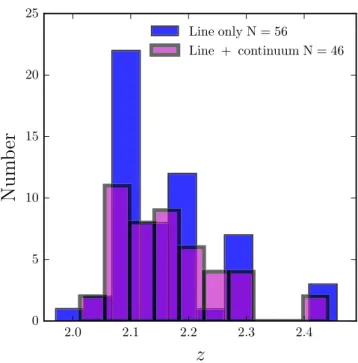
The redshift distribution for the ZFIRE-SP sample is shown by Fig.1. The ZFIRE-SP sample is divided into continuum-detected and non-detected galaxies as described in Section 2.3. Galaxies in our sample lie within redshifts of 1.97<z<2.46 corresponding to at∼650 Myr.

1_{http://zfourge.tamu.edu}

Figure 1. The redshift distribution of the ZFIRE-SP sample. Galaxies with line+continuum detection are shown by magenta and galaxies only with Hα line detection are shown by blue.

2.2 Completeness

In order to determine any significant detection biases in our ZFIRE-SP sample, we evaluate the completeness of the galaxies selected in this analysis. We define a redshift window for analysis between 1.90<z< 2.66 (∼8.6 Gpc), which corresponds to the redshifts that Hαemission will fall within the MOSFIREKband. Note that here we discuss galaxies with Hαdetections and Qz>1, while in

Section 2.1 we discussed the Qz=3 Hα-detected sample.

In the ZFOURGE catalogues used for the ZFIRE sample selection (see Nanayakkara et al.2016for details), there were 1159 galaxies (including star-forming and quiescent galaxies) in the COSMOS field with photometric redshifts (zphoto) within 1.90<zphoto<2.66.

160 of these galaxies with 1.90<zphoto<2.66 were targeted inK

band out of which 1282_{were detected with at least one emission line}

with SNR>5. None of the Hα-detected galaxies had spectroscopic redshifts outside the considered redshift interval. However, three additional galaxies (one object with Qz=2, two objects with Qz=3)

fell within 1.90<z<2.66 due to inaccurate photometric redshifts. There were eight galaxies targeted inKband that did not have Hα detections but do have other emission line detections (i.e. No Hαbut have [NII], [OIII], Hβetc.). Furthermore, there were no galaxies that

were targeted inKband expecting Hαbut resulted in other emission line detections.

There were 151 objects within 1.90< z <2.66 with Hα de-tections (Qz>1) and 26 of them were flagged as AGN following

selection criteria from Coil et al. (2015) and Cowley et al. (2016). In the remaining 125 galaxies, 8 galaxies did not have matching ZFOURGE counterparts and 8 galaxies had low confidence for redshift detection (Qz= 2) from Nanayakkara et al. (2016). We

2_{Note that this is different from the 142 galaxies mentioned in Section 2.1} because the sample of 142 galaxies has a Qz=3, includes galaxies with no ZFOURGE counterparts (see Nanayakkara et al.2016for further details) and galaxies with non-optimal ZFOURGE photometry (see Straatman et al.2016

Nselected: number of ZFIRE-detected galaxies selected for the IMF study with spectroscopic redshifts within 1.90<z<2.66.

Nline only: number of galaxies selected for the IMF study which shows no continuum detection with spectroscopic redshifts within 1.90<z<2.66. Nnull detection: number of ZFIREK-band-targeted galaxies with photometric redshifts within 1.90<z<2.66 and no Hαdetection.

a_{Where applicable spectroscopic redshifts have been used to calculate the stellar masses fromFAST.} b_{One galaxy flagged as an AGN does not have a matching ZFOURGE counterpart.}

removed those 16 galaxies from the sample. Out of the 109 remain-ing galaxies, 7 are removed due to the followremain-ing reasons: 4 galaxies due to negative spectroscopic flux, 1 galaxy due to multiple objects overlapping in the spectra and 2 galaxies due to extreme sky line interference.

Our sample constitutes of the remaining 102 galaxies out of which, 46 have continuum detections (see Section 2.3). Further-more, 38 (out of which 16 are continuum detected) galaxies are confirmed cluster members (Yuan et al.2014) and the remaining 64 (out of which 30 are continuum detected) galaxies comprise of field galaxies. 32 galaxies targeted with photometric redshifts between 1.90<z<2.66 show no Hαemission detection. We divide our sample into three mass bins with masses between log10(M)<9.5,

9.5≤log10(M)≤10.0, 10.0<log10(M) and show the

corre-sponding data as described above in Table1.

We define observing completeness as the percentage of de-tected galaxies (Qz > 1) with photometric redshifts between

1.90<z<2.66 and calculate it to be ∼80 per cent. However, it is possible that the 32 null detections with photometric redshifts within 1.90<z <2.66 to have been detected if the ZFIRE sur-vey was more sensitive. We stack the photometric redshift likeli-hood functions (P(z)) of the ZFIRE targeted galaxies within this redshift range, to compute the expectation of detections based of photometric redshift accuracies (see the Nanayakkara et al.2016

section 3.2 for further details on howP(z) stacking is performed). The calculated expectation for Hαto be detected withinKband is ∼80 per cent, which is extremely similar to the observed complete-ness. Therefore, non-detections rate is consistent with uncertainties in the photometric redshifts. To further account for any detection bias, we employ a stacking technique of the non-detected spectra in order to calculate a lower limit to the stacked EW values. This is further discussed in Section 5.2.

2.3 Continuum fitting and HαEW calculation

In this section, we describe our continuum fitting method for our 102 Hα-detected galaxies selected from the ZFIRE survey. Fitting a robust continuum level to a spectrum requires nebular emission lines and sky line residuals to be masked. Furthermore, the wavelength interval used for the continuum fit should be sufficient enough to

perform an effective fit but should be smaller enough to not to be influenced by the intrinsic SED shape. After extensive testing of various measures used to fit a continuum level, we find the method outlined below to be the most effective to fit a continuum level for our sample.

By visual inspection and spectroscopic redshift of the galaxies in our sample, we mask out the Hαand [NII] emission line regions

in the spectra. We further mask all known sky lines by selecting a region×2 the spectral resolution (±5.5 Å) of MOSFIREKband. We then use the astropy(Astropy Collaboration et al.2013) sigma-clipping algorithm to mask out remaining strong features in the spectra. These spectra are then used to fit an inverse variance weighted constant level fit, which we consider as the continuum level of the galaxy. Three objects fail to give a positive continuum level using this method and for these we perform a 3σclip with two iterations without masking nebular emission lines and sky lines. Using this method we are able to fit positive continuum levels to all galaxies in our sample. We further investigate the robustness of our measures continuum levels in Appendix A using ZFOURGE photometric data and conclude that our measured continuum level is consistent (or in agreement) with the photometry.

We use two approaches to calculate the Hα line flux: (1) di-rect flux measurement and (2) Gaussian fit to sky-line blended and kinematically unresolved emission lines. Our two methods provide consistent results for emission lines that are not blended with sky lines (see Appendix A). By visual inspection, we selected kinemat-ically resolved (due to galaxy rotation etc.) Hαemission lines that were not blended with sky lines and computed the EW by inte-grating the line flux. Within the defined emission line region, we calculated the Hαflux by subtracting the flux at each pixel (Fi) by the corresponding continuum level of the pixel (Fconti). For the

remaining sample, which comprises of galaxies with no strong ve-locity structure and galaxies with Hαemission with little velocity structure and/or Hαcontaminated by sky lines, we perform Gaus-sian fits to the emission lines, to calculate the Hαflux values. We then subtract the continuum level from the computed Hαline flux. Next, we use the calculated Hαflux along with the fitted contin-uum level to calculate the observed HαEW (HαEWobs) as follows:

HαEWobs=

i

1−Fi−Fconti

Fconti

3076

T. Nanayakkara et al.

whereλiis the increment of wavelength per pixel. Finally, using

the spectroscopic redshift (z) we calculate the rest-frame HαEW (αEWrest), which we use throughout the paper:

HαEW= HαEWobs

1+z . (2b)

We calculate EW errors by bootstrap re-sampling the flux of each spectra randomly within limits specified by its error spectrum. We re-calculate the EW iteratively 1000 times and use the 16th and 84th percentile of the distribution of the EW measurements as the lower and upper limits for the EW error, respectively. Since the main uncertainty arises from the continuum fitting, we do not consider the error of the Hαflux calculation in our bootstrap process.

The robustness of an EW measurement relies on the clear identi-fication of the nebular emission line and the underlying continuum level. The latter becomes increasingly hard to quantify at high red-shift for faint star-forming sources due to the continuum not being detected. Therefore, we derive continuum detection limits to iden-tify robustly measured continua from non-detections.

In order to establish the limit to which our method can reliably measure the continuum, we select 14 2D slits with no continuum or nebular emission line detections to extract 1D spectra. We define extraction apertures using a representative profile of the flux moni-tor star and perform multiple extractions per slit depending on their spatial size. A total of 93 1D sky spectra are extracted and their con-tinuum level is measured by masking out sky lines and performing a sigma-clipping algorithm. The error of the sky continuum fit is calculated by bootstrap re-sampling of the sky fluxes 1000 times. We consider the 1σ scatter of the bootstrapped continuum values to be the error of the sky continuum fit and 1σ scatter of the flux values used for the continuum fit as the rms of the flux.

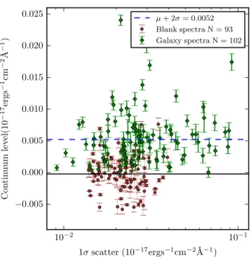
The comparison between the flux continuum levels for the sky spectra with the ZFIRE-SP sample spectra are shown in Fig. 2. The median and the 2σ standard deviation for the continuum lev-els of the sky spectra are −2.3 ×10−21_{erg s}−1_cm−2_Å−1 _and

5.4×10−20_{erg s}−1_cm−2_Å−1_{, respectively. We consider the}

hor-izontal blue dashed line in Fig.2, which is 2σ above the median sky level, to be our lower limit for the continuum detections in our sample. The 46 galaxies in our ZFIRE-SP sample with continuum levels above this flux level detections are considered to have a robust continuum detection. For the remaining 56 galaxies, we consider the continuum measurement as a limit and use it to calculate a lower limit to the HαEW values. The redshift distribution of these galaxies is shown by Fig.1.

2.4 Calculating optical colours

Rest-frame optical colours for the ZFIRE-SP sample are com-puted using an updated version of EAZY3(Brammer et al.2008),

which derives the best-fitting SEDs for galaxies using high-quality ZFOURGE photometry to compute the colours. We investigate the robustness of the rest-frame colour calculation ofEAZYin

Ap-pendix B3. The main analysis of our sample is carried out using optical colours derived using two idealized, synthetic box-car fil-ters, which probes the bluer and redder regions of the rest-frame SEDs. We select these filters to avoid regions of strong nebular emission lines as explained in Section 3 and Appendix B.

In order to allow direct comparison between ZFIREz∼2 galaxies withz=0.1 SDSS galaxies from HG08, we further calculate

opti-3_{Development version:https://github.com/gbrammer/eazy-photoz/}

Figure 2. The figure illustrates the continuum detection levels for the ZFIRE-SP sample. The measured continuum level is plotted against the 1σ scatter of the flux values used to fit the continuum level. The brown circles represent the continuum levels calculated for the blank slits and the green diamonds represent the continuum level calculated for the IMF sample. The blue horizontal line is the 2σ scatter above the median (∼0) for the blank sky regions. Any continua detected above this level of 5.2×10−20_{erg s}−1_cm−2 _Å−1_{are considered as detected continuum levels.}

cal colours for the ZFIRE-SP sample atz=0.1 using blueshifted SDSSgandrfilters. Blueshifting the filters simplifies the (g−r) colour calculation atz =0.1 ((g− r)0.1) by avoiding additional

uncertainties, which may arise due toK-corrections if we redshift the galaxy spectra toz=0.1 fromz=0.

3 G A L A X Y S P E C T R A L M O D E L S

In this section, we describe the theoretical galaxy stellar spec-tral models employed to investigate the effect of IMF, SFHs and other fundamental galaxy properties in Hα EW versus optical colour parameter space. We usePEGASE.2 detailed in Fioc &

Rocca-Volmerange (1997) as our primary spectral synthesis code to per-form our analysis and further employSTARBURST99(S99; Leitherer

et al.1999) and BPASSV2 (Eldridge & Stanway2016) models to

investigate the effects of other exotic stellar features.

PEGASEis a publicly available spectral synthesis code developed

by the Institut d’Astrophysique de Paris. Once the input parameters are provided,PEGASEproduces galaxy spectra for varying time-steps,

which can be used to evaluate the evolution of fundamental galaxy properties over cosmic time.

3.1 Model parameters

In this paper, we primarily focus on the effect of varying the IMF, SFH and metallicity on Hα EW and optical colour of galaxies. A thorough description of the behaviour ofPEGASEmodels in this

off due to the ambiguity of the stellar evolution models above this mass. Varying the upper mass cut-off has a strong effect on Hα EW and optical colours. As HG08 showed this is strongly degener-ated with changing. In this work, we focus onparametrization, noting that changing the cut-off could produce similar effects. We further discuss the degeneracy between the high-mass cut-off and the HαEW versus optical colours slope in Section 6.4.

(ii) The SFH : exponentially increasing/declining SFHs, constant SFHs and starbursts are used. Exponentially declining SFHs are in the form of SFR(t)=p2exp(−t/p1)/p1, withp1varying from 500

to 1500 Myr. Starbursts are used on top of constant SFHs with varying burst strength and time-scales. Further details are provided in Section 5.3.

(iii) Metallicity : models with consistent metallicity evolution and models with fixed metallicity of 0.02 are used.

The other parameters we use for thePEGASEmodels are as follows.

We use Supernova ejecta model B from Woosley & Weaver (1995) with the stellar wind option turned on. The fraction of close binary systems are left at 0.05 and the initial metallicity of the ISM is set at 0. We turn off the galactic in-fall function and the mass fractions of the substellar objects with star formation are kept at 0, Galactic winds are turned off, nebular emissions are turned on and we do not consider extinction as we extinction correct our data.

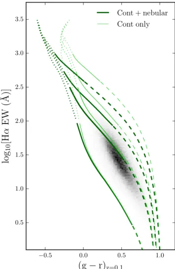
As a comparison with HG08, in Fig.3we show the evolution of four model galaxies fromPEGASEin the HαEW versus (g−r)0.1

colour space. The models computed with exponentially declining SFHs withp1= 1000 Myr, varying IMFs and nebular emission

lines agree well with the SDSS data. However, the evolution of the (g−r)0.1colour shows strong dependence on the nebular emission

contribution, especially for shallower IMFs. HG08 never considered the effect of emission lines in (g−r)0.1colours and the significant

effect at younger ages/bluer colours are likely to be important for

z∼2 galaxies.

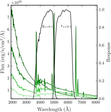
Fig.4shows an example of a synthetic galaxy spectra generated byPEGASE. The galaxy is modelled to have an exponentially

declin-ing SFH withp1=1000 Myr and a= −1.35 IMF. Due to the

declining nature of the SFR, the stellar and nebular contribution of the galaxy spectra decreases with cosmic time. We overlay the filter response functions of thegz₌0.1andrz=0.1filters used in the

analysis by HG08. As evident from the spectra, this spectral region covered by thegz₌0.1 andrz=0.1 filters includes strong emission

lines such as [OIII] and Hβ. Therefore, the computed (g−r)0.1

colours will have a strong dependence on photoionization proper-ties of the galaxies.

To mitigate uncertainties in photoionization models in our anal-ysis, we employ synthetic filters specifically designed to avoid

re-Figure 3. The evolution ofPEGASESSP galaxies in the Hα EW versus (g−r)0.1colour space. We show four galaxy models with exponentially declining SFHs computed using identical parameters but varying IMFs. The thick dark green tracks show from top to bottom galaxies withvalues of −0.5,−1.0,−1.35 and−2.0, respectively. The thin light green tracks follow the same evolution as the thick ones, but the nebular line contribution is not considered for the (g−r)0.1colour calculation. All tracks commence at the top left of the figure and are divided into three time bins. The dotted section of the track corresponds to the first 100 Myr of evolution of the galaxy. The solid section of the tracks show the evolution between 100 and 3100 Myr (z∼2) and the final dashed section shows evolution of the galaxy up to 13 100 Myr (z∼0). The distribution of the galaxies from the SDSS HG08 sample is shown by 2D histogram.

gions with strong nebular emission lines. We design two box-car filters centred at 3400 and 5500 Å with a width of 450 Å. The rest-frame wavelength coverage of these filters corresponds to a similar region covered by the FourStarJ1andHlong filters in the

observed frame for galaxies atz=2.1 and therefore requires negli-gibleK-corrections. Further details on this filter choice is provided in Appendix B1. Henceforth, we refer to the blue filter as [340], the redder filter as [550] and the colour of blue filter−red filter as [340]–[550]. The [340]–[550] colour evolution of a galaxy is independent of the nebular emission lines.

We also compare results usingS99(Leitherer et al.1999) models in Appendix C. We find thatPEGASEandS99models show similar

evolution and find that our choice of SSP model (PEGASEorS99) to

3078

T. Nanayakkara et al.

Figure 4. An example of a model galaxy spectrum generated byPEGASE. Here, we show the evolution of the optical wavelength of a galaxy spectra with an exponentially declining SFH and a= −1.35 with no metallicity evolution. The time-steps of the models from top to bottom are: 100 Myr (dark green), 1100 Myr (green), 2100 Myr (lime green) and 3100 Myr (light green). Thegz=0.1andrz=0.1filter response functions are overlaid on the figure.

introduce rotational and/or binary stars used in these models do have an influence of the HαEWs and [340]–[550] colours, which we discuss in detail in Section 8.4.

3.2 Comparison to HαEW and optical colours atz∼2

We explore the IMF ofz∼2 star-forming galaxies using HαEW values from ZFIRE spectra and rest-frame optical colours from ZFOURGE photometry. Our observed sample used in our analysis is shown in Fig.5. The left-hand panel shows the distribution of Hα EW and [340]–[550] colours of the ZFIRE-SP sample before dust corrections are applied. We overlay model galaxy tracks generated by PEGASEfor various IMFs. All models are computed using an

exponentially declining SFH, but with varying time constants (p1)

as shown in the figure caption. For a given IMF, smoothly varying monotonic SFHs have very similar loci in this parameter space. The thick set of models (third from top) shows a slope with= −1.35, which is similar to the Salpeter slope. Galaxies above these tracks are expected to contain a higher fraction of higher mass stars in comparison to the mass distribution expected following a Salpeter IMF. Similarly, galaxies below these tracks are expected to contain a lower fraction of high-mass stars. Galaxies have a large spread in this parameter space but we expect this scatter to decrease when dust corrections are applied to the data as outlined in Section 4.1.

We note the large scatter of the HαEW values with respect to the Salpeter IMF, especially the large number of high-EW objects (0.5 dex above the Salpeter locus). Could this simply be due to the ZFIRE-SP sample only detecting Hαemissions in bright ob-jects, i.e. a sample bias? First, we note our high completeness of ∼80 per cent for Hαdetections (Section 2.2). Secondly, our Hαflux limits are actually quite faint. To show this explicitly, we define Hα flux detection limits for our sample using 1σ detection thresholds

for each galaxy parametrized by the integration of the error spec-trum within the same width as the emission line. Fig.5(right-hand panel) shows the HαEW calculated using Hαflux detection limits, which illustrates the distribution of the ZFIRE-SP sample if the Hα flux was barely detected. The HαEW of the continuum-detected galaxies decrease by∼1 dex which suggest that our EW detection threshold is not biased towards higher HαEW values.

Similar to IMF, there are a number of effects that may account for the clear disagreement between the observed data and models. In subsequent sections, we explore effects from

(i) dust (Section 4),

(ii) observational bias (Section 4.5), (iii) starbursts (Section 5),

(iv) stellar rotation (Section 6.1), (v) binary stellar systems (Section 6.2), (vi) metallicity (Section 6.3) and (vii) high-mass cut-off (Section 6.4)

in SSP models to explain the distribution of HαEW versus optical colours of the ZFIRE-SP sample without invoking IMF change.

4 I S D U S T T H E R E A S O N ?

As summarized by Kennicutt (1983), the dust vector is nearly or-thogonal to IMF change vector and therefore we expect the tracks in the HαEW versus optical colour parameter space to be independent of galaxy dust properties. In this section, we describe galaxy dust properties. We explain how dust corrections were applied to the data and their IMF dependence and explore the difference in reddening between stellar and nebular emission line regions as quantified by Calzetti et al. (2000) forz∼0 star-forming galaxies.

We useFAST(Kriek et al.2009) with ZFIRE spectroscopic

red-shifts from Nanayakkara et al. (2016) and multiwavelength photo-metric data from ZFOURGE (Straatman et al.2016) to generate estimates for stellar attenuation (Av) and stellar mass for our

galax-ies.FASTuses SSP models from Bruzual & Charlot (2003) and aχ2

fitting algorithm to derive ages, star formation time-scales and dust content of the galaxies. AllFASTSED templates have been

calcu-lated assuming solar metallicity, Chabrier (2003) IMF and Calzetti et al. (2000) dust law. We refer the reader to Straatman et al. (2016) for further information on the use ofFASTto derive SP properties in

the ZFOURGE survey.

4.1 Applying SED-derived dust corrections to data

We use stellar attenuation values calculated byFASTto perform dust

corrections to our data. First, we consider the dust corrections for rest-frame HαEWs and then we correct the [340]–[550] colours.

By using Cardelli, Clayton & Mathis (1989) and Calzetti et al. (2000) attenuation laws to correct nebular and continuum emission lines, respectively, we derive the following equation to obtain dust-corrected HαEW (EWi) values:

log₁₀(EWi)=log10(EWobs)+0.4Ac(V)(0.62f−0.82), (3)

where EWobsis the observed EW,Acis the SED-derived continuum

attenuation andfis the difference in reddening between continuum and nebular emission lines.

Figure 5. The HαEW versus [340]–[550] colour distribution of the ZFIRE-SP sample. No dust corrections have been applied to the observed data. Galaxies with Hαand continuum detections are shown by magenta stars while galaxies only with Hαdetections (and continuum from 1σupper limits) are shown as 1σ lower limits on EW by blue triangles. The errors for the continuum-detected galaxies are from bootstrap re-sampling. The solid (t<3200 Myr) and dashed lines (t>3200 Myr) are SSP models computed fromPEGASE. Similar to Fig.3, we compute models for four IMFs withvalues of−0.5,−1.0,−1.35 (this is the thick set of tracks which is similar to the IMF slope inferred by Salpeter) and−2.0. Each set of tracks from top to bottom represents these IMF in order. For each IMF, we compute three models with exponentially declining SFHs with varyingp1values. From top to bottom, for each IMF these tracks represent

p1values of 1500, 1000 and 500 Myr.Left:the HαEW versus [340]–[550] colours of the ZFIRE-SP sample.Right:similar to the left figure but the HαEW has been calculated using 1σdetection limits of the Hαflux values to demonstrate the sensitivity limits of our EW measurements.

analysis using a dust correction off= 1 to consider equal dust extinction between stellar and ionized gas regions. This is driven by the assumption that A and G stars that contribute to the continuum of

z∼2 star-forming galaxies are still associated within their original birthplaces similar to O and B stars due to insufficient time for the stars to move away from the parent birth clouds within the<3 Gyr time-scale.

Similarly, using Calzetti et al. (2000) attenuation law we obtain dust-corrected fluxes for the [340] and [550] filters as follows:

f([340])=f([340]obs)×100.4×1.56Ac(V) (4a)

f([550])=f([550]obs)×100.4×1.00Ac(V). (4b)

A complete derivation of the dust corrections presented here are shown in Appendix D2.

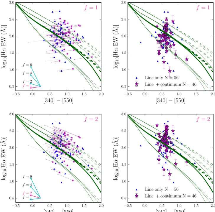
Fig. 6 shows the distribution of our sample before and after dust corrections are applied. In the left-hand panels, we show our sample before any dust corrections are applied, with arrows in cyan

denoting dust vectors for varyingfvalues. It is evident from the figure that the galaxies in this parameter space are very dependent on thefvalue used. Forfvalues of 1 and 2, the effect of dust is orthogonal to IMF change, while values above 2 may influence the interpretation of the IMF. We note thatf>2 makes the problem of high HαEW objects worse, so we do not consider such values further.

3080

T. Nanayakkara et al.

Figure 6. The dust correction process of the ZFIRE-SP sample. This figure is similar to Fig.5but shows the intermediate and final step of the dust correction process.Top left:here, we show the dust correction vector for each galaxy in our sample, computed following the prescriptions explained in Section 4.1. In summary, we use Calzetti et al. (2000) attenuation law to correct the continuum levels and the optical [340]–[550] colours. We use Cardelli et al. (1989) attenuation law to dust correct the nebular emission lines. We use attenuation values calculated byFASTand apply equal amount of extinction to continuum and nebular emission line regions. The purple arrows denote the dust vector for the individual galaxies. Galaxies with no arrows have 0 extinction. The arrows in the bottom left corner show the dust vector for a galaxy withAv=0.5 but with varying Calzetti, Kinney & Storchi-Bergmann (1994) factors, which is shown asfnext to each arrow.Top right:the final HαEW versus [340]–[550] colour distribution of the dust-corrected ZFIRE-SP sample withf=1. Most galaxies lie at ([340]−[550])∼0.6, which corresponds to∼850 Myr of age following the Salpeter IMF tracks.Bottom left:similar to top left panel, but with a higher amount of extinction to nebular emission line regions compared (∼×2) to the continuum levels.Bottom right:the final HαEW versus [340]–[550] colour distribution of the dust-corrected ZFIRE-SP sample withf=2.27.

Even∼×2 larger errors for the individual HαEW measurements cannot account for the galaxies with the largest deviations from the Salpeter tracks. The change offfrom 2⇒1 decreases the median HαEW value by∼0.2 dex. However, galaxies still show a large scatter in HαEW versus [340]–[550] colour parameter space with points lying well above the Salpeter IMF track.

Figure 7. Here, we show the distribution of the ZFIRE-SP sample in the HαEW versus [340]–[550] colour parameter space with the Hαcontinuum and optical colours dust corrections applied followingleft:Calzetti et al. (2000) attenuation law,centre:Pei (1992) SMC attenuation law andright:Reddy et al. (2015) attenuation law. In all panels, Cardelli et al. (1989) attenuation law has been used to dust correct the nebular emission lines with equal amount of extinction applied to continuum and nebular emission line regions (f=1). The arrows in the bottom left corner show the dust vector for a galaxy withAv=0.5 but with varying Calzetti et al. (1994) factors, which is shown asfnext to each arrow.

attenuation curve forz∼2 galaxies atλ2500 Å and a Calzetti et al. (2000)-like attenuation curve for the shorter wavelengths. However,HSTgrism and SED fitting analysis of galaxies atz∼2– 6 has shown no deviation in the attenuation law derived by Calzetti et al. (2000) for local star-forming galaxies. Such conflicts are also apparent in simulation studies, where Mancini et al. (2016) showed evidence for SMC-like attenuation with clumpy dust regions while Cullen et al. (2017) have shown that galaxies contain similar dust properties as inferred by Calzetti et al. (2000).

In order to understand the role of dust laws in the HαEW ver-sus [340]–[550] colour parameter space, we compare the results using other dust laws such as Pei (1992) SMC dust law and Reddy et al. (2015) z ∼ 2 dust law to correct the stellar contributions (Hαcontinuum and optical colours). A comparison between the distribution of galaxies obtained with different dust laws for a givenfis shown by Fig. 7. The fraction of galaxies withEW

>2σ from the= −1.35 IMF track withf=1 (f=2) dust cor-rections are∼20 per cent(∼45 per cent),∼35 per cent(∼75 per cent) and∼15 per cent(∼55 per cent) for Calzetti et al. (2000), Pei (1992) SMC and Reddy et al. (2015) dust laws, respectively. However, we refrain from interpreting the differences in the distributions of the sample between the considered dust laws because the attenuation values used in the ZFIRE/ZFOURGE surveys have been derived from SED fitting byFASTusing a Calzetti et al. (2000) dust law. Compared to the adopted dust law, the change in the value offhas a stronger influence on the galaxies in our parameter space and can significantly affect the EW values, which is discussed further in Section 4.4.

To investigate differences between ourz∼2 sample with HG08

z∼0 sample, we derive dust corrections to the (g−r)0.1colours.

Using the following equations to apply dust corrections tog0.1and

r0.1fluxes we recalculate the (g−r)0.1colours for the ZFIRE-SP

sample.

f(gi)0.1=f(gobs)0.1×100.4×1.25Ac(V) (5a)

f(ri)0.1=f(robs)0.1×100.4×0.96Ac(V). (5b)

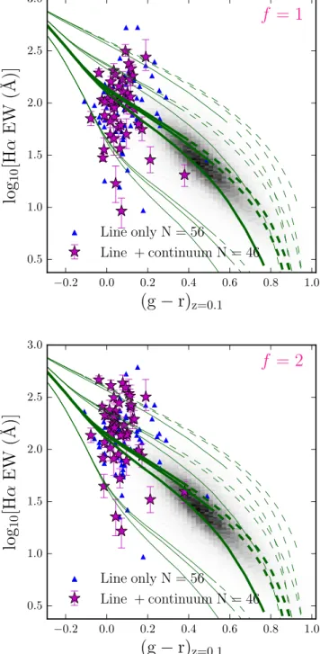
We show the HαEW versus (g−r)0.1colour comparison between

ZFIRE and SDSS samples in Fig.8. The dust corrections for the ZFIRE-SP sample have been performed using anf = 1 and an

f= 2. Similar to the [340]–[550] colour relationship, there is a significant presence of galaxies with extremely high HαEW values and∼60 per cent of the galaxies lie above the Salpeter IMF track when dust corrections are applied with anf=2. Furthermore, the

z∼2 sample shows much bluer colours compared to HG08 sample, which we attribute to the younger ages (∼850 Myr inferred from tracks with a Salpeter IMF) and the higher SFRs of galaxies atz∼2. In Fig.9, we use the= −1.35 IMF tracks to compute the de-viation of observed HαEW values from a canonical Salpeter like IMF. For each (g−r)0.1 galaxy colour, we calculate the expected

HαEW using the standardPEGASEmodel computed using an

ex-ponential decaying SFH with ap1=1000 Myr. We then calculate

the deviation between the observed values to the expected values. Only thef=2 scenario is considered here to be consistent with the dust corrections applied by HG08. Our results suggest that the ZFIRE sample exhibits a lognormal distribution with a mean and a standard deviation of 0.090 and 0.321 units, respectively. Similarly for the HG08 sample, the values are distributed with a mean and a standard deviation of−0.032 and 0.250 units. Compared to HG08, the ZFIRE-SP sample shows a larger scatter and favours higher Hα EW values for a given Salpeter-like IMF. A simple two sample K-S test for the ZFIRE-SP sample and HG08 gives aKsstatistic of 0.37

and aPvalue of 1.32×10−12_{, which suggests that the two samples}

are distinctively different from each other. In subsequent sections, we further explore whether the differences between thez∼0 and

z∼2 populations are driven by IMF change or other SP parameters.

4.2 IMF dependence of extinction values

Dust corrections applied to the ZFIRE-SP sample, as explained in Section 4.1, are derived from FAST (Kriek et al.2009) using

best-fitting model SEDs to ZFOURGE photometric data.FASTuses

a grid of SED template models to fit galaxy photometric data to derive the best-fitting redshift, metallicity, SFR, age and Av

values for the galaxies via a χ2 _{fitting technique. Even though}

these derived properties may show degeneracy with each other (see Conroy2013for a review), in generalFASTsuccessfully describes

observed galaxy properties of deep photometric redshift surveys (Whitaker et al.2011; Skelton et al.2014; Straatman et al.2016).

3082

T. Nanayakkara et al.

Figure 8. Comparison of the HαEW and (g−r)0.1colours of thez∼2 ZFIRE-SP sample with the HG08z∼0 sample. The HG08 sample is shown by the 2D grey histogram. ThePEGASEmodels shown correspond to varying IMFs: from top to bottom= −0.5,−1.0,−1.35 and−2.0. Similar to Fig.5, for each IMF we show three models with exponentially declining SFHs with varyingp1 values (from top to bottomp1 =1500, 1000 and 500 Myr). Model tracks att>3200 Myr are shown by the dashed lines. Top:ZFIRE-SP sample with dust corrections applied with anf=1.Bottom:

ZFIRE-SP sample with dust corrections applied with anf=2. Note that HG08 uses anf=2 in their dust corrections.

cannot explore the effect of varying IMFs on theFAST-derived

ex-tinction values.

In order to examine the role of IMF on derived extinction values, we compare the distribution of ZFIRE rest-frame UV and optical colours withPEGASEmodel galaxies. Following the same procedure

used to derive the [340] and [550] filters, we design two box-car

Figure 9. Deviations of the observed Hαfrom the canonical Salpeter like IMF tracks in the HαEW versus (g−r)0.1 colour space. We show the

z∼0 SDSS HG08 sample (grey–black) and thez∼2 ZFIRE-SP sample (cyan–red). Both histograms are normalized to an integral sum of 1 and the best-fitting Gaussian functions are overlaid. The parameters of the Gaussian functions are shown in the legend.

filters centred at 1500 Å ([150]) and 2600 Å ([260]) with a length of 675 Å. The wavelength regime covered by these two filters approx-imately correspond to theBandIfilters in the observed frame for galaxies atz∼2 (further information is provided in Appendix B2). Therefore, K-corrections are small and the computed values are robust.

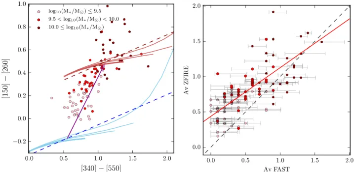
By binning galaxies in stellar mass, we find massive galaxies to be dustier than their less massive counterparts. We show the distribution of our sample in the rest-frame UV versus rest-frame optical parameter space in Fig.10(left-hand panel).PEGASEmodel

galaxies with= −1.35 and varying SFHs are shown by the solid model tracks. When we apply anAv =1 extinction, the models

show a strong diagonal shift due to reddening of the colours in both axis. For each set of tracks, we perform a best-fitting line to the varying SFH models. The dust vector (shown by the arrow) joins the two best-fitting lines drawn to the models withAv = 0 and

Av =1 at timet. We defineAv(ZF) to be the correction needed

for each individual galaxy to be brought down parallel to the dust vector to the best-fitting line withAv=0, and is parametrized by

the following equation:

Av(ZF)= −0.503×([340]−[550])

+1.914×([150]−[260])+0.607. (6)

Our simple method of dust parametrization is similar to the tech-nique used byFAST, which fits SED templates to the UV continuum to

Figure 10. Dust parametrizations to investigate IMF dependences of dust extinction values. Galaxies are divided into three mass bins.Left:the dust content of the galaxies are parametrized using UV/optical colours. The cyan solid lines arePEGASEmodels for= −1.35 IMF with varying SFHs. The dashed blue line is the best-fitting line for these models. The pink lines are similar to the cyan lines, but with an extinction of 1 mag. The magenta dashed line is the best-fitting line for these models withAv=1. The purple arrow denotes the direction of the dust vector and connects the two best-fitting lines at timet.Right:comparison between the extinction derived by equation (6) with the extinction values derived byFAST. The error bars are the upper and lower 68th percentile of theAv values compiled byFASTand the diagonal red line is the error-weighted least-squares fit to the data. The diagonal dashed line is theAv(SED)=Av(ZF) line.

In the right-hand panel of Fig.10, we compare the derived extinc-tion values from our method [Av(ZF)] with the extinction values

de-rived byFAST[Av(SED)]. Since Chabrier (2003) IMF atM∗>1 M

is similar to the slope of Salpeter IMF (= −1.35), the comparison is largely independent of the IMF. The median andσNMADscatter

of theAvvalues derived via FASTand our method is∼−0.3 and

∼−0.3, respectively. Therefore, the values agree within 1σ. There is a systematic bias forAv(ZF) to overestimate the extinction at

lowerAv(SED) values and underestimate at higherAv(SED)

val-ues. We attribute this residual pattern to age metallicity degeneracy, which is not considered in the derivation ofAv(ZF).

The choice of IMF will affect dust corrections derived from UV photometry (usingFASTor our empirical method) as there is a

mod-est dependence of the rmod-est-frame UV continuum slope on IMF for star-forming populations. We are primarily interested in IMF slopes shallower than Salpeter slope ( >−1.35) to explain our popula-tion of high HαEW galaxies. For= −0.5, we find the best-fitting model line in the left-hand panel of Fig.10shifts down by∼0.1 mag. This increases the magnitude of dust corrections and extends the ar-rows in Fig.6to bluer colours and higher EWs and does not explain the presence of high HαEW objects. For the purpose of comparing with our default hypothesis (Universal IMF with= −1.35), we adopt theFAST-derived dust corrections.

4.3 Balmer decrements

Stellar attenuation values computed by fitting a slope to galaxy SEDs in UV, estimates the extinction of old SPs that primarily con-tributes to the galaxy continuum. Nebular emission lines originate from hot ionized gas around young and short-lived O and B stars. Given their short lifetime (∼10–20 Myr), O and B stars are not expected to move far from their birthplace (dusty clouds), thus, the

nebular emission lines are expected to have high levels of extinc-tion. Next, we investigate the dust properties of the stars in different star-forming environments using the luminosity ratios of nebular hydrogen lines and observed UV colours.

Luminosity ratios of nebular hydrogen lines are insensitive to the underlying SP and IMF parameters for a fixed electron temperature (Osterbrock1989). These line ratios are governed by quantum me-chanics and therefore can be used to probe the reddening of nebular emission lines and dust geometry under the assumption that ionized gas attenuation resembles that of the underlying SP.

With the recent development of sensitive NIR imagers and multi-object spectrographs, studies have now started to investigate the properties of dust atz∼2 (Reddy et al.2015; Shivaei et al.2015; de Barros, Reddy & Shivaei2016). These studies show conflicting results on the fraction of stellar to nebular attenuation of galaxies atz∼2. Here, we show Balmer decrement results for a subsample of our ZFIRE-SP sample which shows SNR>5 detections for both Hαand Hβ. The data presented herein are a combination of data released by the ZFIRE data release Nanayakkara et al. (2016) and additional MOSFIRE observations carried out during 2016 January. Our sample comprises of 42 galaxies with both Hαand Hβemission line detections with an SNR>5 and 35 galaxies are part of the ZFIRE-SP sample. Further details on Hβdetection properties are explained in Appendix D1.

3084

T. Nanayakkara et al.

Figure 11. Balmer decrement properties of the ZFIRE sample. Here, we show the subset of Hα- and Hβ-detected galaxies in our ZFIRE-SP sample. The 2D density histogram shows the distribution of values from Reddy et al. (2015)Left:Hβflux versus Hαflux measurements for the ZFIRE-SP sample. The individual galaxies are divided into three mass bins. The diagonal dashed line is thef(Hα)=2.86×f(Hβ) line which denotes the Balmer decrement for case B recombination.Right:comparison between SED-derived extinction values with extinction computed from the Balmer decrement. The black dotted line is theE(B−V)neb=E(B−V)cont/0.44 relationship expected from Calzetti et al. (2000) to compute the extra extinction for nebular emission line regions. The brown dashed line is theE(B−V)neb=E(B−V)contline and the horizontal solid black line is theE(B−V)neb=0 line. Galaxies withE(B−V)neb<0 have been assigned a value of 0.

The colour excess is computed from the Balmer decrement using

E(B−V)neb=

2.5

1.163×log10

_f

(Hα) 2.86×f(Hβ)

. (7)

The distribution of our sample in these panels is similar to Reddy et al. (2015) results as shown by the 2D density histogram and therefore highlights the complicated dust properties ofz∼2 star-forming galaxy populations.

4.4 The difference in extinction between stellar and nebular regions

In this section, we investigate how the differences in dust properties between stellar and ionized gas regions can affect the distribution of our galaxies in HαEW versus [340]–[550] colour space. Calzetti et al. (2000) showed that, forz∼0 star-forming galaxies, the nebular lines are∼×2 more attenuated than the continuum regions, but at

z∼2 studies show conflicting results (Reddy et al.2015; Shivaei et al.2015; de Barros et al.2016). Using ZFIRE data in Fig.11, we show that galaxies occupy a large range of f values in our Hβ-detected sample. We attribute the scatter in extinction to the properties of sight-lines of the nebular line regions.

Since the universe is only∼3 Gyr old atz∼2, the dense molecular clouds collapsed to form stars would only have had limited time to evolve into homogeneous structures within galaxies. This can give rise to differences in the dust geometries within ionizing clouds resulting in non-uniform dust sight-lines for galaxies atz∼2. By varying the value offas a free parameter, we calculate thefvalues

required for our galaxies to be consistent with a universal IMF with slope= −1.35. For each dust-corrected [340]–[550] colour, we compute the Hα EW of the PEGASE = −1.35 IMF track with

p1=1000 Myr. We then use the observed and required HαEW

values to compute thefas follows:

f =

log10(HαEW)=−1.35−log10(HαEW)obs

0.44×0.62×Ac(v)

+0.82 0.62

, (8)

where log10(HαEW)= −1.35 is the HαEW of thePEGASEmodel

galaxy for dust-corrected [340]–[550] colours of our sample and log10(HαEW)obsis the observed HαEW.

In Fig. 12, we show thef values required for our galaxies to agree with a universal IMF with a slope of = −1.35. For the 46 continuum-detected galaxies,∼30 per cent showf<1. It is ex-tremely unlikely that galaxies atz∼2 would havef<1, which suggests that ionizing dust clouds where the nebular emission lines originate from are less dustier than regions with old SPs. Further-more, galaxies that lie above the Salpeter track [log10(HαEW)>

2.2] requiresf<1 and therefore even a varyingfhypothesis cannot account for the high-EW galaxies.∼17 per cent of continuum de-tections havef<0 which is not physically feasible since it requires dust to have the opposite effect to attenuation. Therefore, we reject the hypothesis that varyingfvalues could explain the high HαEWs of our galaxies.

4.5 Observational bias

Figure 12. The distribution offvalues required for galaxies in the ZFIRE-SP sample to agree with a= −1.35 Salpeter like IMF. For each dust-corrected [340]–[550] colour of the ZFIRE-SP sample galaxies, we use the corresponding HαEW of the= −1.35PEGASEtrack with an exponentially declining SFH with ap1=1000 Myr to compute thefvalue required for the observed HαEW to agree with the= −1.35 IMF. The vertical dashed line is thef=0 line.

High HαEW can result due to two reasons:

(i) High line flux: suggests a higher SFR in time-scales of ∼10 Myr.

(ii) Lower continuum level: suggests lower stellar mass for galax-ies.

These two scenarios should be considered together: i.e. a higher line flux with lower continuum level would suggest the galaxy to be going through an extreme star formation phase. We investigate any detection bias that could explain our distribution of HαEWs.

In Nanayakkara et al. (2016), we show that the ZFIRE COSMOS

K-band detections are mass complete to log10(M∗/M)∼9.3. In

Fig.13, we show the distribution of the Hαflux and continuum levels of our sample. It is evident from Fig.13 (left-hand panel) that our galaxies evenly sample the star-forming main sequence described by Tomczak et al. (2014) without significant bias towards extreme Hαflux values. Therefore, we conclude that the Hαfluxes we detect are typical of star-forming galaxies atz=2.1.

In Fig.13 (right-hand panel), we compare our Hαflux values with the derived continuum levels. Continuum-detected galaxies show continuum levels that are in the order of∼2 mag smaller compared to the Hα fluxes and therefore the higher Hα EWs in our sample are primarily driven by the low continua. Note that our continuum detection level is∼−2.3 log flux units. Therefore, for galaxies with only line detection, the difference between Hαflux and continuum level is much higher, which suggests much larger HαEWs.

Several studies investigated the Hα EW of galaxies at higher redshifts (z≥1.5) (Erb et al.2006; Shim et al.2011; Fumagalli et al.2012; Kashino et al.2013; Stark et al.2013; Masters et al.2014; Sobral et al.2014; Speagle et al.2014; Marmol-Queralto et al.2016;

fraction of high-mass stars.

In Section 5, we investigate the effects of starbursts on our study to examine how probable it is for∼1/3rd of our galaxies to have quenched their star formation within a time-scale of10 Myr.

5 C A N S TA R B U R S T S E X P L A I N T H E H I G H Hα E W S ?

Galaxies at z ∼ 2 are at the peak of their SFH (Hopkins & Beacom 2006). We expect these galaxies to be rapidly evolving with multiple stochastic star formation scenarios within their SPs. If our sample consists of a significant population of starburst galax-ies, it may cause significant systemic biases to our IMF analysis.

In this section, we investigate the effects of bursts on the SFHs of the galaxies. We study how the distribution of galaxies in HαEW versus [340]–[550] colour space may be affected by such bursts and how we can mitigate their effects. We demonstrate that our final conclusions are not affected by starbursts.

5.1 Effects of starbursts

A starburst event would abruptly increase the HαEW of a galaxy within a very short time-scale (5 Myr). The increase in ionizing photons is driven by the extra presence of O and B stars during a starburst which increases the amount of Lyman continuum photons. Assuming that a constant factor of Lyman continuum photons get converted to Hαphotons via multiple scattering events, we expect the number of Hαphotons to increase as a proportion to the number of O and B stars. Furthermore, the increase of the O and B stars would drive the galaxy to be bluer causing the [340]–[550] colours to decrease.

The ability of a starburst to drive the points away from the mono-tonic Salpeter track is limited. The deviations are driven by the burst fraction, which we define as the burst strength divided by the length of the starburst. If the burst fraction is small, it has a small effect. However, if it is very large it dominates both the Hαand the optical light, the older population is ‘masked’, and it heads back towards the track albeit at a younger age, i.e. one is seeing the monotonic history of the burst component. The maximum deviation in our study occurs for burst mass fractions of 20–30 per cent occurring in time-scales of 100–200 Myr or fractions of thereof, which can cause excursions of up to∼1 dex. However, as we will see this only occurs for a short time.

We show the effect of a starburst on a PEGASEmodel galaxy

3086

T. Nanayakkara et al.

Figure 13. Here, we investigate which observable parameter/s drive the high HαEW values compared to= −1.35 Salpeter-like IMF expectations in Hα EW versus [340]–[550] colour space.Left:the logarithmic Hαflux of the ZFIRE-SP sample as a function of stellar mass. The Hαflux has been dust corrected following equation (D6a) withf=1/0.44. The black line is derived from the star formation main sequence from Tomczak et al. (2014), converted to Hαflux using Kennicutt (1998b) Hαstar formation law atz=2.1.Right:the Hαflux versus the continuum level at 6563 Å. Both parameters [Hαflux as above, continuum level following equation (D6b)] have been corrected for dust extinction and are plotted in logarithmic space. The Hαfluxes are∼2 orders of magnitude brighter than the continuum levels.

∼3000 Myr generated during the burst) is overlaid on the constant SFH model at time=1500 Myr. The starburst drives the increase of HαEW which occurs in a very short time-scale. In Fig.14, the galaxy deviates from the constant SFH track as soon as the burst occurs and reaches a maximum HαEW within 4 Myr. At this point, the extremely high mass stars made during the burst will start to leave the main sequence. This will increase the number of red giant stars resulting in higher continuum level around the Hαemission line. Therefore, the HαEW starts to decrease slowly after∼4 Myr. Once the burst stops, the HαEW drops rapidly to values lower than pre-burst levels. The galaxy track will eventually join the= −1.35 smooth SFH track at a later time than what is expected by a smooth SFH model.

We further investigate the effect of starbursts with smaller time-scales (tb<20 Myr) and find that the evolution of HαEW in the aftermath of the burst to be more extreme for similarfmvalues. This

is driven by more intense star formation required to generate the same amount of mass within∼1/10th of the time-scale. Since both HαEW and [340]–[550] colours are a measure of sSFR, we expect the evolution to strongly dependent onfmandτbof the burst and to

be correlated with each other.

To consider effects of bursts, we adopt two complimentary ap-proaches. First, we stack the data in stellar mass and [340]–[550] colour bins. SPs are approximately additive and by stacking we smooth the stochastic SFHs in individual galaxies and also account the effect from galaxies with no Hαdetections. Secondly, we use

PEGASEto model starbursts to generate Monte Carlo simulations to

predict the distribution of the galaxies in Hα EW versus [340]– [550] colour space. Using the simulations, we investigate whether it is likely that the observed discrepancy is driven by starbursts and also double check whether the stacking of galaxies would generate smooth SFH models.

5.2 stacking

In order to remove effects from stochastic SFHs of individual galax-ies in our sample, we employ a spectral stacking technique. We first divide the galaxies into three mass and dust-corrected [340]–[550] colour bins as follows.

(i) Mass bins: log10(M∗/M)≤9.5, 9.5<log10(M∗/M)<10, log10(M∗/M)≥10

(ii) [340]–[550] colour bins: ([340]–[550]) ≤ 0.56, 0.56<([340]–[550])<0.65, ([340]–[550])≥0.65

We select a wavelength interval of∼1500 Å centred around the Hαemission for each spectra and mask out the sky lines with ap-proximately 2×the spectral resolution. In order to avoid systematic biases arisen from narrowing down the sampled wavelength region in the rest frame, we instead redshift all spectra to a commonz=2.1 around which most of the galaxies reside. We sum all the spectra at this redshift, in their respective bins. The error spectra are stacked in quadrature following standard error propagation techniques.

We mask out the nebular emission line regions of the stacked spectra and use a sigma-clipping algorithm to fit a continuum (c1). The error in the continuum is assigned as the standard deviation of the continuum values of 1000 bootstrap iterations.

We visually inspect the stacked spectra to identify the Hα emis-sion line profiles to calculate the integrated flux. Stacked HαEW is calculated following equations (2a) and (2b).