THE SKEWNESS IN EXPECTED MACRO FUNDAMENTALS AND PREDICTABILITY OF EQUITY RETURNS: EVIDENCE AND THEORY
Wasin Siwasarit
A dissertation submitted to the faculty of the University of North Carolina at Chapel Hill in partial fulfillment of the requirements for the degree of Doctor of Philosophy in the Department of
Economics.
Chapel Hill 2015
Approved by:
Eric Ghysels
Riccardo Colacito
Anusha Chari Mariano M. Croce
c
2015
ABSTRACT
WASIN SIWASARIT: THE SKEWNESS IN EXPECTED MACRO FUNDAMENTALS AND PREDICTABILITY OF EQUITY RETURNS: EVIDENCE AND THEORY.
(Under the direction of Eric Ghysels and Riccardo Colacito.)
We document that the first and third cross-sectional moments of the distribution of GDP growth rates made by professional forecasters can predict equity excess returns, a finding which is robust to controlling for a large set of well established predictive factors. We show that introducing time-varying skewness in the distribution of expected growth prospects in an otherwise standard endowment econ-omy can substantially increase the model implied equity Sharpe ratios, and produce a large amount of fluctuation in equity risk premia.
ACKNOWLEDGMENTS
There are more than 150,681, 600 seconds (4 years, 9 months, 9days) that I have stayed in Chapel Hill, North Carolina. Undoubtedly, all the scenes, moments, are still vivid and heartfelt every time when I remind to it. I therefore would like to express a deep appreciation to these individuals for their supports and contributions, in one way or the other, to this dissertation.
First and foremost, I am particularly indebted to my remarkably intellectual advisors, Prof. Eric Ghysels and Prof. Riccardo Colacito. I have met them in my second-year classes which are Introduc-tion to Empirical Finance and FoundaIntroduc-tions of Macro-Finance. In summer of that year, I had a great opportunity to work with them for my field paper in financial econometrics. I have learned a lot from working closely with them. After passing the field paper examination, I continued working with them as their advisee. We regularly had the meeting every week to update my research progress. In our meeting environment, we always enjoy solving the problems we found in our research and we always happy with the results we had. During three years that I worked with them, more than 150 meetings in Ric’s office and on Skype calls, I can definitely say that I enjoyed every minute of it!. Thanks so much for being the strong and supportive advisors to me.
I am also very grateful to Prof. Anusha Chari, Prof. Mariano M. Croce, and Prof. Toan Phan, who made innumerable and invaluable comments and suggestions. Taking Prof. Chari ’s class in International Finance and Prof. Croce’s class in Methods in Macro-Finance inspires me in doing the Macro-Finance research. I always recommend the second-year students to take these two classes.
I thank Prof. Pab Jotikasthira for giving me a good opportunity to work as his TA and RA at Kenan-Flagler Business School.
Living in a small city like Chapel hill is boring if I don’t have such groups of friends to do activities together. I am very thankful my writing group at UNC writing center: Dr. Gigi Taylor, Percival Guevarra, Vicky Yeh, Soo Jin Lee, and Geovani Ramirez. I have been especially fortunate to have a chance to know and join the meditation group at UNC: Linda Chupkowski, Christina Lebonville, Lauren Townsend,and Alden Adrion–Thanks so much for your support, friendship, and hospitality.
I want to thank my good friends at department of economics, department of statistics, and depart-ment of finance: Ben, Brian, Melati, Yiyi, Hanwei, Pragya, Derya, Daniel, Laura, Atet, Roberto, Tao, Jinghan, Sunjin.
I owe a special debt to P0Pi, P0Nuch, P0 Kub, Nase, P0 Rong, N0 Paula, and N0 Wai for being my
true friends. Especially, P0Pi, she helped me to accept the sudden loss of my father and travelled back
to U.S with me after I finished with my father’s funeral in Thailand. I also thank my Thais friends that I have made in Chapel hill for their support and friendship.
I thank Linda Longs and her family. It is my privilege to stay with you while I studied here. Your love, care, and support are richly appreciated. I will definitely miss you when I go back to Thailand and will be looking forward to seeing you in Bangkok or when I come back to U.S.
I thank William Young and Madeline Young for being my best host family since my first-year in Chapel hill.
Along with the above people, I wish to express my special thanks to Thammasat University for supporting me with generous fellowships when I studied at University of North Carolina at Chapel Hill.
Finally, I want to offer a special thanks to my family for their love, support, sacrifice, kind indul-gence, and understanding. I also would like to express my sincerest gratitude to my grandmother, my grandfather ,and my father. Although they passed away, their love, support, and care is still in my heart. I own this to them.
All these acknowledgment notwithstanding, responsibility for the dissertation is mine. If any of readers has any comments or suggestions, please bring them to my attention. Any comments will be deeply appreciated.
TABLE OF CONTENTS
LIST OF TABLES . . . ix
LIST OF FIGURES . . . xi
1 INTRODUCTION . . . 1
2 TIME SERIES PROPERTIES OF THE CROSS-SECTIONAL MOMENTS OF THE DISTRIBUTION OF EXPECTED REAL GDP GROWTH RATES . . . 5
2.1 Time series properties of the cross-section of expected GDP growth . . . 6
2.2 Predictive regressions . . . 9
3 THE MODEL . . . 14
3.1 A model with time-varying mean and skewness . . . 14
3.2 A model with time-varying volatility and skewness . . . 18
4 COMPARISON WITH OTHER MODELS . . . 24
4.1 Skewness in consumption based asset pricing models . . . 24
4.2 Asset pricing moments . . . 28
4.3 Sensitivity analysis . . . 31
5 CONCLUSION . . . 35
APPENDIX A Technical Appendix . . . 36
A.1 The skew normal distribution . . . 36
A.2 Solution of the model . . . 37
A.3 Solution for the constant volatility case . . . 39
A.4 Solution of the model with time-varying volatility and skewness . . . 43
A.5 GMM estimation . . . 44
A.6 Conditional moments in the model with jumps . . . 47
A.7 Time series properties for alternative data configurations . . . 48
A.8 Robustness of predictive regressions . . . 49
A.9 Proofs of lemmas . . . 49
A.10 Approximations . . . 77
A.11 Analytical solution of the case with time-varying volatility and skewness . . . 78
A.12 Additional calculations for GMM estimation . . . 89
A.13 Numerical algorithm . . . 94
A.14 Comparison of approximations . . . 97
A.15 Models with jumps . . . 110
LIST OF TABLES
2.1 Time Series Properties of Cross-Sectional Moments . . . 8
2.2 Predictive Regressions . . . 10
2.3 Correlation between Predictors . . . 12
3.1 Calibration . . . 20
3.2 Model Implied Predictive Regressions at Semi-annual Frequency . . . 22
3.3 Correlation of Excess Returns: Quintile Analysis . . . 23
4.1 Monthly Calibration . . . 25
4.2 Comparison of Models . . . 29
4.3 The Role of Skewness in Predictive Regressions . . . 30
4.4 Sensitivity Analysis . . . 33
A.1 Time Series Properties of Cross-Sectional Moments . . . 50
A.2 Predictive Regressions: Livingston + Blue Chip (ALL) . . . 52
A.3 Predictive Regressions:Livingston (cross-sectional size>20) + Blue Chip . . . 54
A.4 Predictive Regressions: Livingston (cross-sectional size>30) + Blue Chip . . . 56
A.5 Predictive Regressions: Livingston + Blue Chip (ALL) with Bootstrap Standard Deviations . . . 58
A.6 Predictive Regressions: Livingston (up to 98) + Blue Chip with Bootstrap Standard Deviations . . . 60
A.7 Predictive Regressions:Livingston (cross-sectional size>20) + Blue Chip with Bootstrap Standard Deviations . . . 62
A.8 Predictive Regressions: Livingston (cross-sectional size>30) + Blue Chip with Bootstrap Standard Deviations . . . 64
A.9 Predictive Regressions: Livingston + Blue chip (ALL) with Kurtosis . . . 66
A.10 Predictive Regressions: Livingston (up to 98) + Blue Chip with Kurtosis . . . 68
A.11 Predictive Regressions:Livingston (cross-sectional size>20) + Blue Chip
with Kurtosis . . . 70
A.12 Predictive Regressions: Livingston (cross-sectional size>30) + Blue Chip with Kurtosis . . . 72
A.13 Predictive Regressions (Delete Overlap from 1990S1-1997S2) . . . 74
A.14 Maximum Percentage Error of Volatility Approximation . . . 77
A.15 Summary Statistics of Consumption Growth Rate . . . 93
A.16 Comparison of Analytical Solutions for the Constant Volatility Case . . . 107
A.17 Comparison of Analytical and Numerical Solutions of Utility Function for Constant Volatility Case . . . 109
A.18 Comparison of Analytical and Numerical Solutions of Log Price-Dividend Ratio for Constant Volatility Case . . . 119
A.19 Comparison of Analytical and Numerical Solutions of Utility Function in the Model with Time-Varying Volatility and Skewness . . . 120
A.20 Comparison of Analytical and Numerical Solutions of Log Price-Dividend Ratio in the Model with Time-Varying Volatility and Skewness . . . 121
LIST OF FIGURES
2.1 Time Series for The First Three Cross-Sectional Moments of The Distribution
of Expected Real GDP Growth. . . 6
3.1 Utility Function. . . 21
4.1 Comparison of Conditional Skewness of Expected Consumption Growth
Across Models. . . 27
CHAPTER 1: INTRODUCTION
Each month a large number of forecasts about expected growth prospects of the economy is made available to the public. A lot of attention is typically devoted to the average or median of these fore-casts, sometimes called the consensus forecast. We document that the cross-sectional moments of the distribution of professional forecasters’ expected GDP growth help predict future equity excess returns. In particular, we show that the first and third cross-sectional moments have economically and statistically significant predictive power, as larger mean and more positive skewness predict lower equity returns going forward. This empirical result remains even after one controls for standard
predic-tors such ascay(as in Lettau and Ludvigson (2001)), dividend yields, default premia, VIX, variance
risk premium, realized variance of the S&P 500 (Bollerslev et al. (2009)) or the so called Fear index (Bollerslev and Todorov (2011)).
The empirical evidence of return predictability for asymmetry poses a serious challenge as stan-dard asset pricing models, which are inherently symmetric, do not feature such patterns. We address this challenge by building a model which mimics the patterns we discover with the aforementioned predictive regressions. We follow Bansal and Yaron (2004) by assuming that investors order con-sumption profiles using Epstein and Zin (1989) preferences. This means that agents care about the temporal distribution of risk. In particular, we show that this type of investors not only likes high expected utility levels and positive asymmetry about future outcomes, but also dislikes uncertainty and negative asymmetry about future wealth.
for future revisions of the conditional mean. In addition to the numerical solution of the model, we provide approximate analytical solutions and show that the latter provide an accurate description of the model’s solution. We also characterize the pricing kernel as a function of the shocks in the model and derive conditional equity risk premia. This allows us to document the predictive power of skewness as determined by our model.
We perform a direct validation of the model, by feeding the actual time-series of mean, volatility, and skewness of analysts’ forecasts in the model’s solution to document that conditional expectations of future returns are quite correlated with future realized returns. Furthermore, we show that the introduction of skewness can: (i) substantially increase equity risk premia, and (ii) produce a large amount of time variation in conditional risk premia. What is also interesting to note is that the theo-retical model we develop not only features time-varying skewness, but attributes a special role to an interaction term of skewness and standard deviation - acting like a signed scaled variance term. The empirical support for this term is even more striking than the actual skewness itself.
We compare the performance of our model relative to the recent strand of the literature that has looked at jumps as a way of introducing tail risk. For example, Bansal and Shaliastovich (2013) present an equilibrium model in which fluctuations in investors confidence about expected growth lead to variation in risk premia. Their economy set-up follows the long-run risks specification of Bansal and Yaron (2004), and features a Gaussian consumption growth process with time-varying expected growth and volatility. In a related paper, Drechsler and Yaron (2011) consider the possibility of jumps in both the level and the volatility of the expected growth rate of consumption. A common feature of these recent models is that the dynamics of the skewness of expected macroeconomic fundamentals is tied to the dynamics of volatility. Our analysis, using a skew-normal distribution with time-varying parameters, allows us to introduce an additional skewness factor, which turns out to be quite important. For example, in the Drechsler and Yaron (2011) model, periods of high volatility are associated to periods of low skewness in absolute value, while times of low macroeconomic uncertainty coincide with an increased amount of left tail risk. The tied link between volatility and skewness makes it difficult for the existing models to match the signs of relevant coefficients in predictive regressions. This feature of the existing models represents a strong argument for including a separate factor to model the dynamics of skewness. Our model does this in a parsimonious fashion and enables us
to match the signs and magnitudes of relevant parameters in predictive regressions, while keeping the skewness factor empirically plausible and tied to the aforementioned cross-sectional moments of expected growth.
This dissertation is related to several strands of the literature. On the empirical side, an extensive literature has documented the predictability of equity excess returns at various horizons (see inter alia Welch and Goyal (2008)). Campbell and Diebold (2009) have provided evidence in support of the predictive power of the consensus forecast for subsequent stock market returns. It is noteworthy that, while the coefficient on average expected growth is always strongly statistically significant, the one on the dispersion is typically not. We extend their findings and show that the degree of asymmetry helps explaining equity returns going forward. Remarkably, asymmetry matters far more than dispersion does, i.e. the third moment matters while the second does not. Furthermore, there is a considerable literature on asset pricing models with investors who take into account higher moments (beyond
vari-ances) inasset returns. Arditti (1967), Rubinstein (1973), Kraus and Litzenberger (1976), and Harvey
and Siddique (2000) developed some of the early models of expected returns which incorporate the higher moments of individual securities that co-move with the aggregate market portfolio. Similarly, Christoffersen and Diebold (2006) emphasize the predictability in asset return signs, and show how it remains valid with time-varying conditional skewness and/or kurtosis.
with positive, and one with negative skewness, whose relative importance varies through time.1 They show that this richer consumption dynamics allows the habits’ model by Campbell and Cochrane (1999) to account for the variance risk premium. We differentiate from these papers by proposing a model in which the dynamics of skewness are anchored to the observed degree of asymmetry of expected macroeconomic forecasts, and that speaks directly to our novel empirical evidence.
Our work emphasizes skewness in fundamentals, but we do not focus necessarily on rare disaster risks (see for example Wachter (2013)). Rather, we highlight the importance of skewness even dur-ing “normal” times. Moreover, our approach does not rely exclusively on negative skewness. Time varying skewness may be both positive and negative: both will matter in our approach. The work by Tsai and Wachter (2014) constitutes a notable exception, as they consider both the possibility of rare disasters and rare booms. Our work differs from theirs in that our skewness process is smoother due to the absence of jumps. Also related is Benzoni et al. (2011) who combine recursive preferences with a very large and rare shock to a persistent component in cash-flow growth rates to generate a steep implied-volatility smirk. In our work the movements in skewness are not simply driven by rare events and provide directional information about either up- or downside risks. Finally, our work is related to Chabi-Yo (2012) and Bakshi and Chabi-Yo (2014) that have pointed out the relevance of higher order moments for the construction of tighter bounds on the variance of pricing kernels.
The dissertation is organized as follows. The next chapter presents our main empirical findings by discussing the time-series properties of the cross-sectional moments of the distribution of expected GDP growth rates, as well as documenting the predictive power of skewness for future stock market returns. Chapter 3 presents a version of our model that can be solved in closed form and that is calibrated to match the time-series properties of the cross-sectional moments of the distribution of expected GDP growth rates. We use this model to explain how skewness affects equity returns and to document the crucial interaction between skewness and volatilities. Chapter 4 performs a comparison between our model and the model with jumps proposed by Drechsler and Yaron (2011). Chapter 5 concludes the work.
1
In a related paper, Bekaert et al. (2015) develop the econometric framework to estimate the “Bad Environment-Good Environment” class of models.
CHAPTER 2: TIME SERIES PROPERTIES OF THE CROSS-SECTIONAL MOMENTS OF THE DISTRIBUTION OF EXPECTED REAL GDP GROWTH RATES
Multiple forecasts are commonly available for key economic variables, as different professional analysts may disagree about the outlook of the economy, or, simply, because different forecasting models and/or information are employed in this task. In this chapter, we put ourselves in the position of an investor who looks at the entire cross-sectional distribution of these forecasts at each point in time. We document that this distribution features time-varying mean, volatility, and skewness. Campbell and Diebold (2009) find that the professional forecasters’ cross-sectional distribution time-varying mean and volatility help predict future stock returns. Their empirical finding can be reconciled with a number of asset pricing models.
What we document next is both empirically novel and theoretically intriguing. We find that the cross-sectional skewness of analyst forecasts predicts future stock returns. The predictability of re-turns using cross-sectional skewness is even stronger than for the first two conditional moments and is robust to the inclusion of both standard predictors as well as commonly used measures of downside and/or distress risks. It is important to note that the cross-sectional skewness is not simply a measure of downside risk - as it also reflects upside growth states.
-4 -2 0 2 4
1955 1960 1965 1970 1975 1980 1985 1990 1995 2000 2005 2010
Mean Skewness Volatility
Figure 2.1: Time series for the first three cross-sectional moments of the distribution of expected real GDP growth. Mean stands for the median forecast, Variance stands for the interquartile measure of volatility (i.e. the 75th percentile less the 25th percentile), and Skewness is the quantile-based measure of skewness (i.e. the 75th percentile plus the 25th percentile minus twice the median). The series are constructed using one semester ahead real GDP growth forecasts from the Livingston and Blue Chip datasets from 1951:1 to 2011:2. The vertical grey bars represent recessions according to the National Bureau of Economic Research.
2.1 Time series properties of the cross-section of expected GDP growth
Dataset. We construct the time series of cross-sectional measures of mean, dispersion, and
asym-metry of real GDP growth expectations by using two datasets.1 The first one is the Livingston Survey,
which starts in 1946 and is the oldest continuous survey of economists’ real GDP growth expecta-tions. It summarizes the forecasts of economists from industry, government, banking, and academia. The Federal Reserve Bank of Philadelphia took responsibility for the survey in 1990. Every June and December, participants forecast a set of key macroeconomic variables, including real and nominal GDP. Survey participants are asked to provide forecasts for three horizons: (1) the end of the current month, (2) six months ahead, and (3) 12 months ahead. For each date we have a cross-section of up
1Since 1968 a richer data set that includes individual density forecasts is available. To motivate the theory and build our
empirical models we opted for the longer time series with only the individual point forecasts.
to 50 forecasts. Our interest in this specific survey is motivated by the fact that it spans the longest time period, an appealing feature since we are trying to capture the properties of a slowly moving component of GDP growth.
The second dataset is given by the Blue Chip Economic Indicators. Each month this dataset provides forecasts up to one and a half years ahead. It is available starting in 1984. The dataset consists entirely of analysts affiliated with the financial services’ industry. We merge this dataset with the Livingston Survey by restricting our attention to the two quarters ahead forecasts of real GDP growth rates made in June and December of each year. This has at least two benefits: it increases the cross-sectional size for part of our sample, and it compensates for the drop in the number of analysts that the Livingston Survey experiences in the late 1990’s and that continues for about five years. By combining the two datasets, we have an average cross-sectional size in the order of 70, which allows for a greater degree of precision in the estimation of the cross-sectional moments.
Time varying moments. Figure 2.1 reports the time series for the first three cross-sectional moments
of the distribution of expected GDP growth rates.2 The figure shows that these moments are
vary-ing over time. While average expected GDP growth is on average positive, the skewness is typically negative. The dispersion of the forecasts appears to be very persistent. Quite interestingly, the three moments appear to be mutually uncorrelated. This suggests that the asymmetry of the distribution of forecasts may contain additional information about the risk factors in the economy. A qualitative finding that can be appreciated from looking at Figure 2.1 is that skewness tends to turn more nega-tive right before the beginning of recessions, even at times when the mean forecast would otherwise suggest normal growth rates. This effect is particularly apparent for the last two recessions.
Time series regressions. Table 2.1 reports some additional information about the time series proper-ties of the cross-sectional moments of the distribution of average forecasts. Since the cross-sectional size of the Livingston Survey drops from 44 in the second semester of 1998 to 31 in the first semester of 1999, and it reaches a minimum of 19 in 2004, we conduct our analysis by combining the Livingston survey up to 1998, and the the Blue Chip survey over their entire sample. In the Online Appendix, we
2
Table 2.1: Time Series Properties of Cross-Sectional Moments
Persistence VAR analysis
Mean Volatility 3rd Mom1/3 Mean Volatility 3rd Mom1/3
Lagged Mean 0.499 − − 0.471 −0.021 −0.025
(0.07) (0.056) (0.017) (0.051)
Lagged Volatility − 0.914 − 0.312 0.877 −0.256
(0.057) (0.248) (0.048) (0.136)
Lagged 3rd Mom1/3 − − 0.307 0.436 −0.088 0.257
(0.086) (0.124) (0.037) (0.074)
Notes - Time series properties of cross-sectional moments. The panel labeled “Persistence” reports the estimates of the AR(1) coefficients for the mean, volatility, and third centered moment to the power of 1/3. The panel labeled “VAR analysis” reports the estimates of time series regressions of each variable on the corresponding column and the three lagged variables reported in the rows. The numbers in brackets underneath each estimate are heteroskedasticity adjusted standard errors.
conduct the analysis on five alternative datasets: the results are robust across data configurations (see Table A.1 in the Online Appendix).
In the panel labeled “Persistence”, we estimate three separate AR(1) processes for the mean, the
volatility, and the third centered moment to the power of1/3. We choose to focus on this specific
power of the third moment, because the model that we propose in the later sections directly imposes restrictions on its dynamics. Our time series estimates suggest that all three moments feature statisti-cally significant first order autocorrelations. The persistence appears to be more pronounced for the first two moments.
The panel labeled “VAR Analysis” further investigates the dynamics by including the lags of all three cross-sectional moments as right hand side variables of the regressions. The interesting finding is that the third moment seems to have predictive power for the conditional mean. More specifically our estimates indicate that following periods of positive asymmetry, the conditional mean increases. This property of the conditional skewness will prove itself important in our theoretical analysis, as news to the shape of the distribution of forecasts will matter in forming the entire stream of future growth prospects.
2.2 Predictive regressions
We explore the predictive content of the first three cross-sectional moments of GDP growth fore-casts for equity excess returns, measured as the logarithmic returns on the S&P500 index minus the returns on three months Treasury bills. Equity prices are obtained from Robert Shiller’s website, while
Treasuries are obtained from the web site of the Federal Reserve Bank of St. Louis.3
Predictive regressions. Table 2.2 reports the results of our predictive regressions. In all the specifica-tions, we regressed the ex-post six months excess returns on the ex ante cross-sectional moments of the distribution of real GDP growth rate, and on some additional variables that are known to have
pre-dictive power for equity returns. In the table,E[growth]stands for the median forecast,V[growth]
stands for the interquartile measure of volatility (i.e. the75thpercentile less the25thpercentile), and
S[growth]is the quantile-based measure of skewness (i.e. the75thpercentile plus the25thpercentile minus twice the median). Part of our results confirm the findings of Campbell and Diebold (2009), in that positive average expected GDP growth rates significantly forecast lower future returns, while the opposite is true for the measure of dispersion of forecasts. Furthermore, while the coefficient on aver-age expected growth is always strongly statistically significant, the one on the dispersion is typically not.
Panel A in Table 2.2 covers cross-sectional moments at the beginning of each six months interval from 1952 to 2010, using the cross-sectional moments of the distribution of real GDP growth rate
in addition to the following predictors: cay, the term premium, the dividend yield, and the default
spread taken from Lettau and Ludvigson (2001). The latter are variables known to have predictive power for equity returns. Panel B adds a number of recently proposed predictive regressors, which are
only available for a shorter sample from 1990 to 2010, namely the VIX2, the variance risk premium
(denoted VRP) and realized variance of the S&P 500 (denoted RV) are from Bollerslev et al. (2009).4
It also contains the Fear index constructed by Bollerslev and Todorov (2011) which starts in 1996.
3
The dataset is available athttp://www.econ.yale.edu/ shiller/data/chapt26.xls.
Table 2.3: Correlation between Predictors
V[growth] S[growth] cay default term pr. DP VIX2 VRP RV fear
E[growth] −0.352 −0.148 −0.044 −0.254 0.247 −0.263 −0.649 −0.206 −0.583 −0.237
V[growth] −0.076 −0.122 0.109 −0.278 0.616 0.622 0.159 0.576 0.231
S[growth] 0.044 0.087 −0.013 −0.105 0.346 0.204 0.265 0.168
cay −0.100 0.274 0.006 −0.133 0.228 −0.248 0.353
default 0.149 0.301 0.814 −0.046 0.875 0.418
term pr. −0.290 0.134 0.044 0.120 0.434
DP 0.006 −0.155 0.080 0.241
VIX2 0.325 0.893 0.510
VRP −0.134 0.427
RV 0.309
Notes - The table reports the correlation between equity return predictors.E[growth],V[growth], andS[growth]refer to the median, volatility, and skewness of the cross-sectional distribution of expected GDP growth rate at the beginning of each six months interval from 1952 to 2010. The predictorscay, the default spread, the term premium, and the dividend yield are from Lettau and Ludvigson (2005), from 1952 to 2010. VIX2, VRP and RV are from Bollerslev, Tauchen and Zhou (2010), from 1990 to 2010. Fear is from Bollerslev and
Todorov (2011) starting in 1996.
Table 2.3 reports the correlations across the set of variables that we include in our predictive
re-gressions. The first striking observation is the relatively low correlation betweenS[growth]and the
commonly used predictors, namely less than 10 % withcay, the default spread, the term premium
and marginally higher with the dividend yield. The correlations are higher but still moderate with
the recently proposed risk measures. In particular with VIX2the correlation is the highest at almost
35 %. Interestingly, other measures pertaining to downside risk, such as the Fear index yield only a
low correlation of 17 %. The latter is important to recognize as it shows thatS[growth]is measuring
both upside as downside skewness - as indicated in Figure 2.1. In contrast,V[growth]features much
stronger correlations with dividend yields and volatility related predictors. Moreover, the conditional meanE[growth]also has strong correlations with the standard regressors and surprisingly large
cor-relations with VIX2 and RV. Last, but not least it is also worth noting from Panel A in Table 2.1 that
among the three survey-based moment measuresS[growth]features the lowest persistence, which is
relevant for the econometric analysis of predictive regressions.
For the longest historical data set, we find in Panel A of Table 2.2 that both E[growth] and
S[growth]significantly predict stock returns at a six month horizon according to columns [1]-[3].
Note also thatV[growth]is not significant and that the conditional mean yields the highest adjusted
R2.The fact that skewness has predictive power for future equity returns is intriguing. The negative
sign of the regression coefficient is also intuitive: a more negative asymmetry suggests an increase in
tail risk, and equity holders require extra compensation for it. Conversely, a right-skewed asymmetry lowers the equity risk premium - hence the importance of the role played both by left and right skew-ness. While it is clear from column [2] that the cross-sectional variance is not significant, it is worth
noting - as the result in column [4] indicates - that the interaction termS[growth]1/3∗V[growth]1/2
is significant. The new theoretical asset pricing models discussed later in the dissertation will feature this term. The fact that it is empirically significant will be an implication supported by the data. As indicated in column [5] we also find that the interaction term combined with the cross-sectional first moment yields the best fit and improves the significance of both predictors. In contrast, when the
interaction term is combined with eitherV[growth]orS[growth]we find that it is the interaction
term which matters. The results in column [12] further validate this with a regression model which includes all regressors discussed so far.
How does this evidence stand up against other traditional future return predictors? Columns [8] through [11] and [13] indicate that skewness remains significant when traditional return predictors are either added one by one, or jointly to the specification of the predictive regressions.
Panel B of Table 2.2 documents that the results get even stronger if we include predictors proposed in recent years - although they only apply to shorter samples due to data availability. It is
notewor-thy that the Fear index becomes insignificant when paired withS[growth]1/3∗V[growth]1/2.While
VIX2, VRP and RV remain significant, the latter two become insignificant when combined in a
re-gression with the skewness term, as reported in column [13]. It should also be noted that the best model in Panel B only involved survey-based cross-sectional moments - i.e. the model appearing in column [5]. Finally, as reported in section A.8 of the Online Appendix we find similar results when we pool all the Livingston and Blue Chip survey data.
CHAPTER 3: THE MODEL
In this chapter we introduce our model with time-varying skewness. Our model features a rep-resentative agent that uses the cross-section of analysts’ forecasts to discipline her predictions about the conditional moments of expected GDP growth rates. This chapter consists of two parts. First, we analyze a version of the model without any exogenous time variation in volatility. This version of the model can be solved in closed form, and it allows us to highlight some of the key features pertaining the introduction of skewness in a consumption based asset pricing model. In the second half of this chapter, we relax the assumption of no time variation in volatility. In the context of this generalized version of the model, we perform a number of exercises that document the relevance of the interaction between volatility and skewness.
3.1 A model with time-varying mean and skewness
Preferences. A representative agent maximizes her lifetime utility, which is defined recursively as
Ut= (1−δ) logCt+
δ
1−γ logEt[exp{(1−γ)Ut+1}] (3.1)
whereCtstands for consumption at datet,γmeasures the relative risk aversion (henceforth RRA), and
δis the subjective discount factor. They correspond to Epstein and Zin (1989) preferences for the case
of unit intertemporal elasticity of substitution (henceforth IES).1We choose to restrict our attention
to the case of unit IES for multiple reasons. First of all, empirical estimates of the IES, as surveyed by Havranek (2014), are typically around this value. Second, we can derive closed form solutions for the models presented in this section, when preferences are described by equation (3.1). Additionally,
1
Colacito and Croce (2013) have shown that in a general equilibrium multi-country economy an EIS close to 1 is needed in order to account for several stylized facts of international asset prices and quantities.
The main departure from the constant RRA case often analyzed in the literature lies in the fact that these preferences allow agents to be risk averse in future utility as well as future consumption. The extent of such utility risk aversion depends on the preference for early resolution of uncertainty
measured byγ −1>0. To better highlight this feature of the preferences, it is convenient to look at
a third order expansion of the utility function yields2
Ut ≈ (1−δ) logCt+δEt[Ut+1] +
δ(1−γ)
2 Vt[Ut+1] +
δ(1−γ)2
6 Et
h
(Ut+1−Et[Ut+1])3
i .
This approximation, which we use only for the purpose of characterizing the economic intuition of
the model, highlights several important aspects of our specification. Whenγ = 1, the agent is
utility-risk neutral and preferences collapse to the standard expected utility case. However, for levels of utility-risk
aversion in excess of1, our investor cares also about smooth future utility (lowVt[Ut+1]), and she
dislikes negative skewness of her future utility profile.
The variance and negative skewness aversion are specific to this type of preferences and they suggest that skewness of future growth prospects may matter through a variety of channels in our economy. In this dissertation, we focus on a class of models in which consumption growth is pre-dictable. In particular, we analyze a specification for the dynamics of the predictable component of consumption growth rates in which news about expected future growth prospects are drawn from a skewed distribution, a prediction that conforms well with the empirical evidence reported in chap-ter 2.
Endowments. The investor is endowed with a stochastic supply of the consumption good
∆yt+1 =µc+xt+ √
σεct+1, εct+1∼N(0,1) (3.2)
whereµcis the unconditional mean of∆yt+1,σdenotes the conditional variance of∆yt+1, andxtis
modeled as a highly persistent AR(1) process,
xt+1 = ρxxt+ϕe √
σεxt+1. (3.3)
We assume that the sequence of shocksεxt+1isi.i.d.distributed as a Skew-Normal with shape
param-eterφt+1. Specifically, the probability distribution function ofεxt+1is
2·√1 2π exp
−(ε
x t+1)2
2
| {z }
Normal pdf
·
Z √φt+1 1−φ2t+1ε
x t+1 −∞
1 √
2π exp
−(t)
2
2
dt
| {z }
Normal CDF
.
In words, the probability ofεx corresponds to the probability associated to a standard normal
distri-bution tilted by shaping factor, which depends onφ. Whenφ = 0, the standard normal distribution
attains. Whenφ > 0(φ < 0, respectively), the probability of positive (negative) realizations of εx
is overweighted (underweighted) relative to the probability of negative (positive) realizations of the shock. This effect is due to the cumulative distribution function being monotonically increasing in its
argument, and it generates time-varying skewness in the distribution of the shockεx, as long as the
parameterφvaries over time. We model the dynamics ofφt+1as an AR(1) process:
φt+1 =ρφφt+ √
σφεφt+1, ε φ
t+1 ∼N(0,1) (3.4)
whereρφmeasures the first order autocorrelation ofφt+1, andσφis the conditional variance ofφt+1.
This distribution allows for values of skewness which are bounded between−1and1. Garcia and
Manzanares (2007) employ the skew-normal to analyze the empirical distribution of European pro-fessional forecasts of macroeconomic variables.
Financial Markets and Equilibrium. We assume that there is a complete set of state and date
contingent securities. In equilibrium, the agent consumes her endowment: ∆ct+1 = ∆yt+1. The
pricePtof any asset associated to the sequence of stochastic cash flows{Dj}∞j=tis determined by the
Euler equationPt =Et[Mt+1(Pt+1+Dt+1)], whereMt+1 is the unique stochastic discount factor
(henceforth SDF) that satisfies
Mt+1=
∂Ut/∂Ct+1
∂Ut/∂Ct
.
SDF and equity returns. In Appendix A.3, we document that the Campbell and Shiller (1988) approximation yields a very tractable solution of the model. We show that the logarithm of the SDF can be written as
mt+1−Etmt+1 =−
1−1 θ
√
¯
σεct+1+Vφ √
σφ
θ ε
φ t+1+
Bϕe √
¯ σ
θ ε
x
t+1, (3.5)
where
B = δ
1−δρx
, Vφ=
0.8ϕeBδρφ 1−δρφ
√ ¯
σ , θ= 1
1−γ.
We will typically calibrate the preference parameterγ to be in excess of1. This means that, as long
as the dynamics ofxtandφtare stationary (i.e.ρx <1andρφ < 1), the loadings onεφt+1 andεxt+1
in equation (3.5) are going to be negative. This highlights that securities that pay-off in times of high
economic growth (largeεc), high expected growth (largeεx), or high skewness of expected growth
(largeεφ) will have large expected returns.
We further investigate the relationship between equity risk premia and skewness, by calculating the returns associated to the stochastic cash flow
∆dt=µc+λ
xt−1+
√ ¯
σ εct+√σd √
¯
σ εdt, εdt ∼N(0,1).
Absent the shock εdt, the dividend process would consist of a claim to levered consumption.3 We
introduce the shockεdt to break the otherwise perfect correlation between consumption and dividend
growth rates. We document our calibration below.
We show in section A.2 of the Technical Appendix that the conditional equity risk premium is equal to
Et
h
rdt+1−rft i
= ¯r−αK1(λ−1) 1−K1ρx
ϕe √
¯
σρφ·φt (3.6)
whereα > 0is related to the slope of the normal cdf,K1 ∈ (0,1)is the slope of the Campbell
and Shiller (1988) approximation and all other parameters are defined in the setup of the economy.4
Equation (3.6) documents an important feature of our model. The degree of skewness of expected
eco-nomic growth, indexed byφt, predicts future equity returns. In particular, times of positive (negative)
skewness are associated with a decline (rise) in expected returns. In section A.14 of the Appendix we document that this result is robust to a variety of alternative approximations and numerical solutions.
3.2 A model with time-varying volatility and skewness
In this section, we are interested in better understanding the interaction between time-varying skewness and time-varying volatility, which plays a key role in the predictive regressions presented in chapter 2. To this end, we generalize our baseline model, by introducing an exogenous process for volatility.
Setup of the model. We modify the setup of the model presented in the previous section by replacing
the constant variances (denoted as ¯σ) in equations (3.2) and (3.3) with the following time-varying
variance process:
σt = σ¯(1−ρσ) +ρσσt−1+
√
σεσt, εσt ∼N(0,1). (3.7)
whereσ¯denotes the unconditional mean of the volatility process,ρσmeasures its persistence, andσis
the conditional mean ofσt. Equation (3.7) allows us to incorporate time-varying economic uncertainty
in the dynamics of the model. We use this autoregressive specification because it allows us to compare the performance of our model with some of the related models in this literature, including Bansal and Yaron (2004) and Drechsler and Yaron (2011) (see chapter 4 for this analysis).
4In section A.14.1 of the Appendix we document that the coefficient in front ofφ
tis always negative for several alternative
approximations.
Calibration. We use GMM to estimate the parameters governing the dynamics of xt, σt, and φt.
Specifically, we define
b
Etcs(∆ct+1) =
1 n
n
X
i=1
Eti(∆ct+1) (3.8)
b
Vtcs(∆ct+1) =
1 n
n
X
i=1
h
Eti(∆ct+1)−Ebtcs(∆ct+1) i2
b
Stcs(∆ct+1) = 1 n
Pn i=1
h
Eti(∆ct+1)−Ebtcs(∆ct+1) i3
b Vcs
t (∆ct+1)
3/2
as the cross-sectional mean, variance, and skewness of the distribution of analysts’ forecasts. We estimate paramaters by minimizing the distance between the means, the variances, and the
autocorre-lations of the processes in equations (3.3), (3.4), and (3.7) and the cross-sectional moments in (3.8).5
In the interest of space, all details are reported in Appendix A.5.
The estimated parameters are presented in Table 3.1 along with the associated standard errors. The column labeled “Model” reports the coefficients that we use for our baseline calibration, and it documents that they are all well within the conventional confidence intervals of the estimated
param-eters. Additionally, we calibrate the preference parameters γ and δ to10 and0.993, respectively.
These numbers are in line with what typically encountered in the asset pricing literature (see inter
alia Bansal and Yaron (2004) and Colacito and Croce (2011)). The remaining parametersµc,ϕe,λ,
andσdare calibrated to target average growth rates of consumption and dividend of1.6%per year,
a moderate degree of first order autocorrelation of consumption and dividend growth rates (0.05and
0.1, respectively), and a less than perfect correlation between consumption and dividend growth rates
(0.65in our model).6
5
We note that the processφt is related to the cross-sectional skewnessSbtcsthrough the transformation b Acst q
K2
φ+2(Abcst )2/π
,
whereAbcst =
Et(xt+1−Et(xt+1))3 Vt(x3t+1/2)
1/3
.
6
In the data the point estimate of the correlation between consumption and dividend growth is0.36with a standard error of0.2over the sample for which we have analysts’ forecasts. Bansal and Yaron (2004) report a point estimate of0.55
Table 3.1: Calibration
Panel A:dynamics of mean, variance, and skewness
Parameter Description Model GMM
ρx AR coefficient of the expected consumption growth rate 0.690 0.540
(0.073)
¯
σ Unconditional variance of the short-run shock 3.13×10⁻⁴ 3.85×10⁻⁴
(4.44×10⁻⁵)
√
σε Conditional volatility of the variance of the short-run shock 1.50×10⁻⁴ 2.81×10⁻⁴
(4.89×10⁻⁵)
ρσ AR coefficient of the variance of the short-run shock 0.464 0.407
(0.075)
√
σφ Conditional volatility of skewness 0.425 3.644
(1.796)
ρφ AR coefficient of skewness 0.307 0.185
(0.087)
Panel B:other parameters
Parameter Description Model
γ Risk aversion 10
δ Subjective discount factor 0.993
µc Average consumption growth 0.008
ϕe Ratio of long-run shock and short-run shock volatilities 0.200
λ Leverage coefficient 4.500
σd Scale parameter of dividends’ volatility 28
Notes - Panel A reports the calibration of the parameters associated to the transition dynamics ofxt,σt, and φt(column labeled “Model”), along with the GMM estimated values (column labeled “GMM”). The numbers
in parenthesis are the standard errors of the estimated coefficients. Panel B reports the calibration of all the remaining parameters of the model. The calibration is set to semi-annual frequency.
Interaction between skewness and volatility. A key feature of the stochastic discount factor with recursive preferences is that it reflects news to the future wealth of the representative agent.
Fig-ure 3.1(a) shows the utility function, a measFig-ure of agents’ wealth, as function of σt and φt. This
utility can take on a large range of values as the conditional skewness and volatility explore the state space. Figure 3.1(b) reports three horizontal cuts of the utility function. The middle line refers to the case of zero skewness. This is a version of the Bansal and Yaron (2004) model. Notice that in this case utility is not extremely sensitive to changes in volatility, given that our chosen calibration postulates a very small amount of time-varying volatility. The situation is very different for the cases in which skewness is positive or negative. The interaction between second and third moments produces larger movements in total discounted utilities. As the degree of asymmetry becomes more and more positive, volatility is welfare increasing as it implies a larger probability of landing in an extremely good state of the economy. The opposite is true for the case of negative skewness, since more volatility increases the likelihood of a left tail event. The interaction between time-varying volatility and skewness is
#10-4 8 6
variance <
4 2 0 -1 -0.5
skewness ?
0 0.5 1.312 1.3125 1.313 1.3135 1.314 1.3145
1
value function
variance < #10-4
0 1 2 3 4 5 6 7
value function
1.3124 1.3125 1.31315 1.3138 1.3142
skewness ?=0
skewness ?=-0.89
skewness ?=0.89
Figure 3.1: Utility function. The left panel reports the utility function, Vet = Vt−xt, as a function of the
skewness and of the variance parameters. The right panel shows three slices ofVetfor different
values of skewness.
therefore an important determinant of risk in this economy.
Quantitative performance. We perform two exercises to assess the performance of our model. The first one consists in replicating the type of regressions presented in chapter 2, in the context of our model. Specifically, we simulate our model using the calibration reported in Table 3.1 and regress the
excess returns on equity onto the lagged values ofxt,
√
σt,σt,φt,φ2t, and
√
σtφt. Table 3.2 presents
our results.
The table documents that not only the model produces the right signs for all the coefficients of interest, but also that the magnitudes are very close to the ones that we estimated in the data. Since the
log-linear approximation of the model suggests thatxtshould not predict future returns, we report the
results with and without includingxtas a regressor. The table shows that the results are unaffected by
the inclusion of this variable.
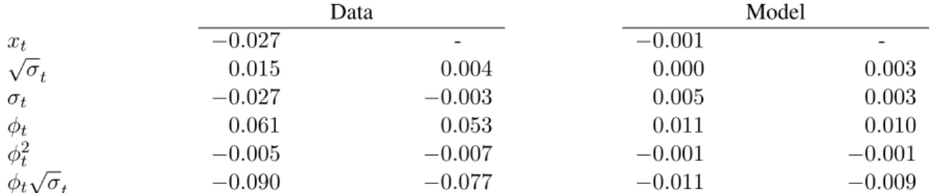
Table 3.2: Model Implied Predictive Regressions at Semi-annual Frequency
Data Model
xt −0.027 - −0.001
-√
σt 0.015 0.004 0.000 0.003
σt −0.027 −0.003 0.005 0.003
φt 0.061 0.053 0.011 0.010
φ2t −0.005 −0.007 −0.001 −0.001
φt √
σt −0.090 −0.077 −0.011 −0.009
Notes -The columns labeled “Empirical Data” report predictive regressions of ex-post six months return on the S&P500 index in excess of the risk free rate. xt,σt,φtare constructed using the cross-sectional moments of
expected GDP growth rate at the beginning of each six months. The columns labeled “Model” report predictive regressions for model implied equity excess returns using semi-annual calibration. The results are obtained from simulating the models 1000 times with sample size equal to 60 years (120 periods). All independent variables are standardized by subtracting their unconditional means and dividing by their standard deviations.
of the conditional risk premium in our model.7 . We then calculate the correlation between these
expected returns predicted by the model and the actual subsequent excess returns in the data. To better characterize the relevance of skewness, we compute the same set of correlations for a version of the model in which any time-variation in skewness has been shut down. Table 3.3 reports the results of our analysis.
We perform this analysis by looking at the five quintiles of the distribution of skewness (the
φt process). The row labeled “Benchmark” in Panel A of Table 3.3 reports the correlations for the
baseline version of our model featuring time-variation in both variance and skewness. The row labeled “No skewness” refers instead to a version of the model with only time-variation in volatility (i.e. the
model that attains by replacing equation (3.4) withφt = 0,∀t). A comparison between the two sets
of correlations highlights that the model that takes into account time-variation in the asymmetry of expected growth rates performs consistently better than its direct competitor. The row labeled “% change” documents that correlations can be even more than twice as large in the benchmark version of our model. Furthermore the improvement in correlations is particularly apparent for the more extreme quintiles of the distribution of skewness. This conveys the idea that our model helps refining the forecast of future returns in times in which the degree of asymmetry of expected macroeconomic fundamentals is more pronounced.
7In the interest of space, we describe all the details is section A.4 of the Technical Appendix.
Table 3.3: Correlation of Excess Returns: Quintile Analysis
Panel A:Correlations by Skewness based Quintiles
Q1 Q2 Q3 Q4 Q5
No Skewness 0.096 0.126 0.325 0.073 0.122
Benchmark 0.219 0.155 0.327 0.092 0.141
% Change (128.6%) (23.3%) (0.8%) (26.0%) (16.0%)
Panel B:The Role of Volatility
Q1 Q2 Q3 Q4 Q5
Lowσt 0.157 −0.319 0.086 0.131 −0.099
Highσt 0.101 0.402 0.289 0.209 0.228
Notes - The table reports the correlations between expected log-excess returns from the model and six months ahead realized excess return on S&P 500 index in each of the five quinteles of the distibution of skewness. The quintiles are labeled as Q1 through Q5. The time series ofσt andφtare constructed using the
cross-sectional moments of the distribution of the growth rate of real GDP expectations from the Livingston and Blue Chips datasets. In Panel A, we report the correlations with the model presented in section 3.2 (labeled as “Benchmark”) and the correlations with the same model with the exception of the time-variation in skewness being shut down (label as “No Skewness”). The row label “% Change” reports the percentage increase in correlations across the two versions of the model. Panel B reports the breakdown of the correlations in Panel A, row labeled “Benchmark” with respect to volatility. The row labeled “Lowσt” refers to the sample in which the
volatility is below its median value, while the row labeled “Highσt” refers to the sample in which the volatility
is above its median value. The sample is 1951:1 to 2010:1.
Panel B of Table 3.3 sheds light on the importance of the interaction between volatility and skew-ness. For each quintile of the distribution of skewness, we decompose the correlation between pected returns in the model and future realized returns into periods of below median volatility of
ex-pected growth rates (row label “Lowσt”) and periods of above median volatility of expected growth
rates (row labeled “Highσt”). The table documents that the correlation is typically larger in periods
CHAPTER 4: COMPARISON WITH OTHER MODELS
In this chapter we perform a comparison of our model with other existing model in the literature. The common feature of all these models lies in their ability of generating large equity risk premia through tail risk in the postulated consumption and cash flow dynamics. We document, however, that time-varying skewness operates in very different ways across models. This is reflected in their comparative performance as far as the predictive regressions are concerned.
The chapter is organized as follows. First, we document the different behavior of skewness in our model relative to the class of models featuring jumps in volatility (as in Bansal and Shaliastovich (2011) and Drechsler and Yaron (2011)). Second, we document the quantitative performance of all these models for a large set of asset pricing moments, and for the predictive regressions discussed in chapter 2. We conclude this chapter with a sensitivity analysis of our model.
4.1 Skewness in consumption based asset pricing models
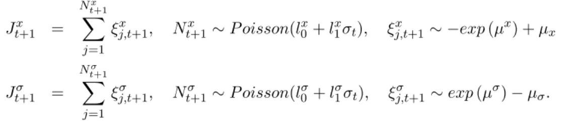
We consider a comparison between our model and some alternative ways of introducing time varying skewness in expected consumption growth rates. Specifically, we focus on the class of models with jumps in volatility and in expected consumption growth of the type discussed in Drechsler and Yaron (2011), Bansal and Shaliastovich (2010), and Bansal and Shaliastovich (2011).
Table 4.1: Monthly Calibration
Panel A:Common Parameters
Parameter Description
ρx AR coefficientxt 0.955
¯
σ Unconditional variance ofσt 4.62×10⁻⁵
ρσ AR coefficient ofσt 0.93
√
σε Conditional volatility ofσt 5.10×10⁻⁶
µc Average consumption growth rate 0.0008
ϕe Scale parameter of long-run volatility 0.050
λ Leverage coefficient 3
σd Scale parameter of dividends’ volatility 20.25
γ Risk aversion 10
δ Subjective discount factor 0.998
Panel B:Model Specific Parameters
Parameter Description Jumps Skew-Normal
µx Location parameter of exponential distribution ofξtx 3.645ϕe
√
¯
σ
lx
0 Constant term of the jump intensity ofJtx+1 0
l1x Loading onσtfor the jump intensity ofJtx+1 0.8/12/σ¯
µσ Location parameter of exponential distribution ofξtσ 2.55 ¯σ
lσ0 Constant term of the jump intensity ofJtσ+1 0
lσ
1 Coefficient in front ofσtfor the jump intensity ofσt 0.8/12/σ¯
√
σν Conditional volatility of the skewness processνt 0.470
ρν AR coefficient of the skewness processνt 0.80
Notes -The table reports the choice of parameters for the monthly calibration of the model. Panel A shows the calibration of the parameters that are in common between the model with skew-normal innovations and the model with jumps. Panel B shows the remaing model specific parameters. The parametersµx,lx0, andlx1control the dynamics of the jumps toxt. The parametersµσ,lσ0, andlσ1 control the dynamics of the jumps to volatility. The parametersρν and
√
σν denote the autocorrelation and volatility of the processνt=φt/ p
1−φ2
t, which
controls the dynamics of skewness.
∆ct+1 = µc+xt+ √
σtεct+1 (4.1)
∆dt+1 = λ∆ct+1+
√ σd
√ σtεdt+1
xt+1 = ρxxt+ϕe
p
σtxεxt+1+Jtx+1
σt+1 = (1−ρσ)¯σ+ρσσt+ √
σεεσt+1+Jtσ+1
σxt = σt 1−2(Et[φt+1])2/π
−1
Skew-Normal,
εxt+1 ∼SKN(0,1, φt+1),
andJtx+1andJtσ+1are modeled as jump processes
Jtx+1 = Nx
t+1 X
j=1
ξj,tx+1, Ntx+1∼P oisson(lx0 +lx1σt), ξj,tx+1 ∼ −exp(µx) +µx
Jtσ+1 = Nσ
t+1 X
j=1
ξj,tσ+1, Ntσ+1∼P oisson(lσ0 +l1σσt), ξj,tσ +1∼exp(µσ)−µσ.
Clearly, by setting the skew-normal parameterφtequal to0for allt, the jump dynamics of the
Drech-sler and Yaron (2011) model attains. DrechDrech-sler and Yaron (2011) also consider the case in which the
jump size of theJtx+1 process is normally distributed. Since this model features by construction a
constant skewness, we will abstract from discussing it in the remainder of this section. By setting the
jump processesJtx+1andJtσ+1to zero delivers the benchmark consumption dynamics presented in this
dissertation. Note that in both models, the variance dynamics is entirely accounted by theσtprocess.
We obtain this by adjusting the variance of the conditional mean process,σtx, to eliminate the effect
of skewness on volatility (last equation of the system in (4.1)).
Table 4.1 reports our baseline calibration. We calibrate the model to describe a monthly decision problem, consistently with the frequency choice of Drechsler and Yaron (2011). We choose to cal-ibrate the parameters that are in common to all models as in Drechsler and Yaron (2011), while the dynamics of the skewness process are chosen in a way to be consistent to the semi-annual moments
reported in chapter 3.1
Figure 4.1 highlights the very different dynamics of the conditional skewness of expected con-sumption growth produced by our model and by the model with jumps. Since the model with nor-mally distributed jumps does not feature any time-variation in skewness, we will focus our attention on the model with negative exponential jumps. The figure documents that the two models have sharply
1
The persistence of the process that controls the dynamics of skewness needs to be set to a larger value to reflect the monthly nature of the calibration. To preventφtfrom hitting its bounds, we specify the AR(1) dynamics onνt =φt/
p 1−φ2
t,
which takes values on the entire real line.
time
0 50 100 150 200 250 300 350 400
Conditional skewness
-10 -9 -8 -7 -6 -5 -4 -3 -2 -1 0 1
Skew-Normal (Benchmark) Negative Exponential Jumps Normal Jumps
Figure 4.1: Comparison of conditional skewness of expected consumption growth across models. The thick line represents our benchmark model with skew-normally distributed innovations. The dashed line refers to the model with jumps with negative exponential innovations. The dash-dot line (the zero line) is the conditional skewness in the model with normally distributed jumps.
different predictions as far as the range of values of skewness is concerned, as well as its degree of persistence and volatility. Note that our benchmark model appears to more closely resemble the magnitude and extent of time-variation of skewness that we presented in chapter 2.
Furthermore, we can characterize the specifictimingof skewness in the model with jumps. Given
the affine nature of the model with jumps, it is easy to show that both variance and third central
moment of xt in the Drechsler and Yaron (2011) model depend linearly on σt. Specifically, we
document in Appendix A.6 that
Vt[xt+1] = (ϕ2e+l1xµ2x)σt, and Et
h
(xt+1−Et[xt+1])3
i
=−2µ3xlx1σt. (4.2)
This has important implications for our model. First of all, it highlights that variance and skewness do
not have independent effects: once equity returns are regressed on the conditional variance ofxt, the
be an increasing function ofσt:
Skewnesst[xt+1] =−
2µ3xlx1 (ϕ2
e+lx1µ2x)3/2 1 √
σt
.
This means that equity risk premia are going to be an increasing function of skewness, the same way they are positively related to variance. This finding is generally at odds with our empirical results, and it calls for an additional risk factor that allows us to disentangle variance from skewness. Our model with time-varying Skew-Normal innovations represents one such model.
4.2 Asset pricing moments
In Table 4.2 we report several asset pricing moments for our benchmark model, the model with jumps, as well as for a number of alternative specifications. For comparison, we report the actual moments calculated using annual US data from 1950 to 2012 obtained from Robert Shiller’s web site in the first column. The results are obtained from simulating the models 1000 times with sample size equal to 100 observations.
Several results ought to be noticed. First of all, a comparison between the specifications in columns 2 and 3, and the specification in column 1 reveals that the introduction of skewness de-termines a large increase in the average equity risk premium. This increase comes together with more volatile equity excess returns, and substantially larger equity Sharpe ratios. Second, the average risk free rate is almost unaffected by the introduction of skewness dynamics. Its volatility increases in the two skewness calibrations, but the 95% confidence intervals (reported underneath each estimate) re-veal that these increases are well within the margin of significance. Third, the average price-dividend ratio is even closer to the data thanks to the introduction of the time-varying skewness process, and so are its volatility and autocorrelation. Table 4.2 also documents the ability of all the models to replicate the almost null amount of skewness of equity excess returns, risk-free rates, and price-dividend ratios. The next two columns (labeled 4 and 5) report the asset pricing moments associated to two al-ternative specifications of our benchmark model model. In column 4, we compensate the change in
T able 4.2: Comparison of Models [1] [2] [3] [4] [5] [6] Data Benchmark No Sk ewness No Sk ewness Adjusted Mean Ne g ati v e Sk ewness D Y Jump Model w/ Constant V ol d t − r
f ]t
4 . 84 5 . 49 1 . 91 3 . 81 2 . 14 8 . 98 3 . 67 (1 . 90) [2 . 54 , 8 . 44] [ − 0 . 08 , 4 . 64] [1 . 17 , 6 . 45] [ − 0 . 57 , 4 . 85] [6 . 26 , 11 . 71] [0 . 71 , 6 . 63] − r
f ]t
16 . 40 18 . 11 13 . 70 13 . 67 14 . 12 14 . 17 15 . 72 (1 . 75) [15 . 58 , 20 . 63] [11 . 75 , 15 . 65] [11 . 66 , 15 . 68] [12 . 04 , 16 . 20] [12 . 09 , 16 . 25] [12 . 15 , 19 . 29] ew [ r
d −t
r
f ]t
0 . 65 0 . 03 0 . 00 0 . 01 0 . 01 0 . 03 0 . 01 (0 . 23) [ − 0 . 42 , 0 . 49] [ − 0 . 48 , 0 . 48] [ − 0 . 50 , 0 . 53] [ − 0 . 47 , 0 . 50] [ − 0 . 46 , 0 . 53] [ − 1 . 21 , 1 . 23]
f ]t
1 . 75 2 . 23 2 . 23 2 . 22 2 . 23 2 . 42 2 . 15 (0 . 50) [1 . 37 , 3 . 09] [1 . 73 , 2 . 74] [1 . 71 , 2 . 73] [1 . 74 , 2 . 72] [1 . 78 , 3 . 06] [1 . 35 , 2 . 94] ] 2 . 30 2 . 02 1 . 23 1 . 23 1 . 19 1 . 50 1 . 87 (0 . 3) [1 . 57 , 2 . 48] [0 . 94 , 1 . 51] [0 . 95 , 1 . 50] [0 . 93 , 1 . 45] [1 . 14 , 1 . 86] [1 . 23 , 2 . 50] ew [ r
f ]t
− 0 . 74 − 0 . 02 0 . 01 − 0 . 03 − 0 . 04 0 . 19 − 0 . 58 (0 . 35) [ − 0 . 63 , 0 . 59] [ − 0 . 55 , 0 . 58] [ − 0 . 65 , 0 . 59] [ − 0 . 68 , 0 . 59] [ − 0 . 48 , 0 . 87] [ − 1 . 89 , 0 . 73] ] 3 . 43 3 . 02 4 . 40 3 . 47 4 . 19 2 . 53 3 . 55 (0 . 26) [2 . 97 , 3 . 08] [4 . 37 , 4 . 43] [3 . 45 , 3 . 50] [4 . 16 , 4 . 22] [2 . 49 , 2 . 57] [3 . 51 , 3 . 59] ] 0 . 43 0 . 16 0 . 09 0 . 09 0 . 10 0 . 11 0 . 12 (0 . 12) [0 . 13 , 0 . 18] [0 . 08 , 0 . 11] [0 . 08 , 0 . 11] [0 . 08 , 0 . 11] [0 . 09 , 0 . 13] [0 . 09 , 0 . 15] ew [ p/d ] 0 . 36 0 . 03 − 0 . 03 − 0 . 04 − 0 . 04 0 . 04 − 0 . 46 (0 . 89) [ − 0 . 41 , 0 . 47] [ − 0 . 50 , 0 . 45] [ − 0 . 55 , 0 . 47] [ − 0 . 54 , 0 . 47] [ − 0 . 50 , 0 . 59] [ − 1 . 63 , 0 . 70] 1 [ p/d ] 0 . 97 0 . 41 0 . 28 0 . 27 0 . 26 0 . 36 0 . 36 (0 . 23) [0 . 21 , 0 . 61] [0 . 06 , 0 . 49] [0 . 06 , 0 . 49] [0 . 05 , 0 . 47] [0 . 15 , 0 . 57] [0 . 12 , 0 . 59] -The first column reports the statis tics of interest calculated using annual US data from 1950 to 2012.The numbers in the parentheses underneath each are the associated standard de viations. The second column reports the results from the model using the benchmark calibration. The column labeled Sk ewness w/Constant V ol” refers to the benchmark calibration with √ σ ν and ρν equal to zero, and constant σt . The column labeled “No Sk ewness” to the benchmark calibration with √ σ ν and ρν equal to zero. The column labeled “Adjusted Mean” refers to the benchmark calibration with the term e √ σ t q
2 Eπ
Table 4.3: The Role of Skewness in Predictive Regressions
Benchmark Model Model with jumps
[1] [2] [3] [4] [5] [1] [2] [3] [4] [5]
(Vt)1/2 0.013 - - - - 0.074 - - -
-(0.003) (0.006)
Vt - 0.013 - - 0.014 - 0.083 - - 0.096
(0.003) (0.003) (0.004) (0.016)
St - - -0.065 - - - - 0.023 -
-(0.003) (0.004)
(St)1/3·(Vt)1/2 - - - -0.129 -0.138 - - - -0.068 0.015
(0.003) (0.003) (0.006) (0.010) Notes -The table reports the models implied predictive regressions for equity excess returns. Panel A refers to the benchmark model in which shocks are skew-normally distributed. Panel B refers to the model with jumps in which the size is distributed as a negative exponential. All variables are standardized by subtracting their unconditional means and dividing by their standard deviations. The results were obtained by simulating the model at a monthly frequency. All standard errors are adjusted for heteroskedasticty.
the conditional mean ofxtthat is due to having time-variation in the conditional skewness.2
Equiva-lently, we shut down the relationship between skewness and future expected GDP growth rates. The results document that the performance of the model is much closer to the one featuring constant skew-ness. This result suggests that the superior performance of our benchmark model is mostly driven by the interaction between time-varying skewness and future expected growth rates. In the fifth col-umn, we alter our benchmark specification by centering the skewness process around a negative value. The table documents that a negative average skewness enhances all the asset pricing predictions of the model. This means that we can interpret our benchmark model, in which skewness is on average equal to zero, as a conservative assessment of the asset pricing implications of time-varying skewness.
The performance of the model with jumps is featured in the last column of Table 4.2. It is apparent that our benchmark model and the Drechsler and Yaron (2011) model perform equally well when it comes to accounting for the unconditional asset pricing moments. The key difference between the two models lies in their predictions for the relationships between variance, skewness, and conditional risk premia. We explore this feature of the models in Table 4.3.
The table is divided into two parts. The first five columns (labeled “Benchmark Model”) report several predictive regression of future excess returns onto lagged moments of the distribution of ex-pected consumption growth. The next five columns (labeled “Model with Jumps”) present the same set of regressions for the model with jumps.
2
This is obtained by adding−ϕe
√
σt
p
2/πEtφt+1to the dynamics ofxtin the system of equations in (4.1).