Single- and Multiple-Shell Uniform Sampling
Schemes for Di
ff
usion MRI Using Spherical Codes
Jian Cheng
∗, Dinggang Shen, Pew-Thian Yap
∗, and Peter J. Basser
∗Abstract—In diffusion MRI (dMRI), a good sampling scheme is important for efficient acquisition and robust reconstruction. Diffusion weighted signal is normally acquired on single or multiple shells in q-space. Signal samples are typically distributed uniformly on different shells to make them invariant to the orientation of structures within tissue, or the laboratory co-ordinate frame. The Electrostatic Energy Minimization (EEM) method, originally proposed for single shell sampling scheme in dMRI, was recently generalized to multi-shell schemes, called Generalized EEM (GEEM). GEEM has been successfully used in the Human Connectome Project (HCP). However, EEM does not directlyaddress the goal of optimal sampling, i.e., achieving large angular separation between sampling points. In this paper, we propose a more natural formulation, called Spherical Code (SC), to directly maximize the minimal angle between different samples in single or multiple shells. We consider not only continuous problems to design single or multiple shell sampling schemes, but also discrete problems to uniformly extract sub-sampled schemes from an existing single or multiple shell scheme, and to order samples in an existing scheme. We propose five algorithms to solve the above problems, including an incremental SC (ISC), a sophisticated greedy algorithm called Iterative Maximum Overlap Construction (IMOC), an 1-Opt greedy method, a Mixed Integer Linear Programming (MILP) method, and a Constrained Non-Linear Optimization (CNLO) method. To our knowledge, this is the first work to use the SC formulation for single or multiple shell sampling schemes in dMRI. Experimental results indicate that SC methods obtain larger angular separation and better rotational invariance than the state-of-the-art EEM and GEEM. The related codes and a tutorial have been released in DMRITool 1.
Index Terms—Sampling, q-space, Multiple Shells, Uniform Spherical Sampling, Diffusion MRI, Spherical Codes
I. Introduction
Diffusion MRI (dMRI) is a unique imaging methodology to explore white matter structure and architecture in the human brain by measuring diffusion of water molecules. In dMRI, signal measurements are a limited number of samples of the diffusion signal E(q) in 3Dq-space. Reconstruction in dMRI entails fitting the signal samples by using a well-designed model, including Diffusion Tensor Imaging (DTI) [1], and
J. Cheng and P.-J. Basser are with SQITS, NIBIB, NICHD, National Institutes of Health. (Emails: [email protected], [email protected])
D. Shen and P.-T. Yap are with the Department of Radiology and Biomed-ical Research Imaging Center (BRIC), the University of North Carolina at Chapel Hill. D. Shen is also with Department of Brain and Cognitive Engineering, Korea University, Seoul 02841, Republic of Korea. (Emails: [email protected], [email protected])
∗denotes the corresponding authors.
Copyright (c) 2017 IEEE. Personal use of this material is permitted. However, permission to use this material for any other purposes must be obtained from the IEEE by sending a request to [email protected].
1https://diffusionmritool.github.io/tutorial qspacesampling.html
various models in High Angular Resolution Diffusion Imaging (HARDI) [2]–[10]. After model fitting, meaningful quantities can be estimated, including diffusion tensor and fractional anisotropy in DTI [1], the ensemble average propagator, dif-fusion Orientation Distribution Function (dODF), fiber ODF (fODF), and the Generalized Fractional Anisotropy (GFA) in HARDI [2]–[9], etc. An appropriate data sampling scheme in
q-space is important for all such dMRI acquisition and recon-struction applications in order to recover as much information as possible by using a minimal number of measurements.
The optimal sampling scheme that yields the best recon-struction quality is dependent on the diffusion model, recon-struction algorithm, and the ground truth diffusion signal. 1) A typical DTI sampling scheme is a single shell scheme with about 30 samples and a low b value (≤ 1200 s/mm2) [11], while multi-shell schemes are preferred (or necessarily needed in some cases) with a higher maximal b value (≥2000 s/mm2) in HARDI methods [4], [5], [9], [10]. 2) Even for the same diffusion model, different reconstruction algorithms, including least squares, robust non-linear estimation with various regu-larizations, etc., may have different preferred schemes [12]. For a given diffusion model, there may be several model fitting (e.g., reconstruction) algorithms. Robust estimation may prefer larger b values due to its robustness to noise [13], [14], and compressed sensing based reconstruction could reduce the number of data samples, compared with traditional least square based reconstruction [15], [16]. 3) Different variabilities of DWI signals may prefer different schemes. An efficient scheme should allocate more samples in the domains with larger signal changes than in domains with smaller signal changes. Error propagation analysis showed that the optimal b value for DTI is inversely proportional to the mean diffusivity of the latent signal [11]. Therefore, it is infeasible to develop a general optimal sampling scheme that works best for all signal variabilities and all reconstruction methods. However, a necessary property for an optimal sampling scheme is that the samples should be spherically uniformly distributed with no directional preference, because 1) an optimal sampling scheme should be invariant to the orientation of tissue structures and the laboratory coordinate frame in which the data is scanned; 2) we have to design one single scheme for all different variabilities of signals in human brain. Thus, existing works [11], [17]–[24] focus on designing single or multiple shell spherically uniform sampling schemes with input param-etersS,{Ks}Ss=1, whereS is the number of shells andKs is the
number of samples in thes-th shell. These parameters are user-determined based on the consideration of diffusion signals, models, reconstruction algorithms, noise level, and the scan
time limit.
Uniform single shell sampling schemes are widely used in dMRI, where samples inq-space are uniformly distributed on a sphere (i.e., a fixed b-value). Spherical tessellation using spher-ical polyhedrons can generate uniform single shell schemes with some specific fixed numbers of samples determined by polyhedron types [2]. On the other hand, the Electrostatic Energy Minimization (EEM) method proposed in dMRI by Joneset al., [11] is the most popular way to generate a uniform single shell sampling scheme with an arbitrary number of samples. EEM considers the samples as electrons on sphere, and estimates the sample configuration by minimizing the electrostatic energy based on Coulomb’s law:
min
{ui}Ki=1
X
i<j
f2(ui,uj), fα(ui,uj)=
1 kui−ujkα2
+ 1
kui+ujkα2 , (1)
where the second term in fα(ui,uj) is used because antipodal
symmetric samples provide redundant information in dMRI data reconstruction. The problem in Eq. (1) is the so-called Thomson problem2. Some best known solutions of EEM have been collected in CAMINO [25]. For the multi-shell case, recently it was reported that staggered samples in different shells are better for reconstruction, compared with repeated spherical samples in different shells [17]–[20], [24]. [19] and [20] tried to design a multi-shell scheme withS shells by separating a single shell scheme into S subsets respectively in different ways to minimize the electrostatic energy. [24] proposed to a rotate single shell scheme and use the rotated scheme in different shells. [17] and [18] generalized EEM from the single shell case to the multiple shell case, called Generalized EEM (GEEM), by considering the electrostatic energies both in each individual shell and in the combined shell with all samples. The obtained multi-shell schemes by GEEM showed large angular separations in shells than [19], [20], and have been successfully used in the Human Connectome Project (HCP) [26]. Although EEM and GEEM are widely used, the electrostatic energy formulation does not directly maximize the angular separation between measurements. Samples in q -space are not electrons, and it is still not clear how electrostatic energy relates to dMRI reconstruction.
A good sampling scheme should have large angular separa-tion such that the reconstrucsepara-tion has large angular resolusepara-tion and good rotational invariance. Thus we propose a mathemat-ically more natural way for sampling scheme design, which directly maximizes the minimal angular difference between sampling points, i.e.,covering radius, on the unit sphere. This way to determine sample configuration on sphere is essentially called the Spherical Code (SC) formulation3, or Tammes prob-lem 4. In many diffusion MRI applications, the information redundancy is considered in local spatial neighborhoods and local angular neighborhoods [27]–[30], which is based on a natural assumption that if the samples ui anduj are close in
the sphere, then the DWI signal samples E(qui) and E(quj)
are also close. Thus, based on this assumption, maximizing the
2http://en.wikipedia.org/wiki/Thomson problem
3http://mathworld.wolfram.com/SphericalCode.html 4https://en.wikipedia.org/wiki/Tammes problem
separation angles between nearest sampling points is related to minimizing the information redundancy in measured DWI samples. The SC formulation directly maximizes the minimal separation angles between the nearest samples. While in the EEM formulation, the electrostatic energy is determined by distances between all sample pairs, not just the nearest sam-ples. Moreover, the covering radius (i.e., minimal separation angle between samples) is a natural and direct measurement of “angular resolution” of spherical sampling schemes, compared with the electrostatic energy. Some pioneer works of HARDI uses finer tessellation gradient table (i.e., larger number of samples with smaller separation angles) to investigate the non-Gaussianity of DWI signals [2], [31]. Wedeenet al., [32] used
q
4π
K to roughly measure the angular resolution of schemes.
Caruyer et al., [17], [18] evaluated schemes by different methods using the covering radius. Thus, it is natural to directly maximize the covering radius of sampling schemes.
SC is related with the famous thirteen spheres problem
raised by Isaac Newton, and has been well studied in math-ematics [33]–[35]. T´oth [33] proved an upper bound for the covering radius of K samples on a sphere. There is also a collection of best known solutions for the SC problem with the antipodal symmetry constraint in S2 [34] 5. It can be proven that the SC problem is equivalent to EEM problem in Eq. (1) whenα→ ∞. Thus, Papadakiset al., [36] tried to approximately solve SC problem by iteratively increasing α in Eq. (1). However asαincreases, the optimization problem has more local minima and becomes more unstable because the cost function tends to be discontinuous and floating-point overflow occurs [36]. Since the SC formulation directly maximizes the minimal distance between samples, it yields larger angular separation than EEM formulation. However to our knowledge, the SC formulation and the collected best known solutions have not yet been used in the dMRI domain. Although SC is well-studied in the mathematical literature, its current formulation is limited to a continuous single shell, and is not applicable to multiple shells, nor to the discrete problem to uniformly extract subsets from an existing scheme.
In this paper, we propose the SC formulation in diffusion MRI with total five algorithms, not only for continuous prob-lems to design single and multiple shell schemes, but also for discrete problems to uniformly sub-sample an existing scheme, and for ordering an existing scheme. Preliminary parts of this work were reported in two conference papers [37], [38]. In this paper, we categorize sampling scheme design problems in dMRI, propose total 5 algorithms in a unified framework of minimizing the mean covering radius, and provide additional examples, results, derivations, and insights.
The paper is organized as follows. Section II proposes the SC formulation and shows how the existing sampling scheme design problems in dMRI can be formulated as optimization problems using SC. Section III proposes 5 algorithms to solve the problems in Section II. Section IV demonstrates some experimental results of synthetic data and real data.
II. SphericalCode(SC)andSamplingProblems inDMRI
A. Spherical Code (SC) Formulation
For a given set of spherical samples{ui∈S2}Ki=1, we define
the covering radius 3 for thei-th sample as
di({ul}Kl=1)= minj ,i,∀j
arccos|uTiuj|. (2)
where the absolute value operator is used because the antipodal symmetric samples have the same role in dMRI data recon-struction. We also define the covering radiusfor all samples as the minimal angular distance between all sample pairs, i.e.,
d({ul}Kl=1)=mini di({ul}Kl=1)= min
j,i,∀i,∀jarccos
|uTiuj|, (3)
The SC formulation on a single shell is to find K samples {ui}Ki=1 such that the covering radius is maximized:
max
{ui∈D}K i=1
d({ui}iK=1) (4)
where D ⊆ S2 is the solution domain. If
D = S2, Eq. (4) is a continuous SC (CSC) problem for selecting K points from the continuous sphere S2. If
D = {un}Nn=1, a set of N predetermined points on S2, then Eq. (4) is a discrete SC (DSC) problem for selectingK fromN points. For CSC, [34] proposed to iteratively optimize a continuous cost function that approximates the original cost function in Eq. (4). The authors also released a collection of best known solutions for the SC problem in S2 [34]5. Note that the original SC problem only considers CSC, i.e., D =S2, while in this paper we propose both CSC and DSC formulations and generalize them to multi-shell case for designing sampling schemes in dMRI.
For multi-shell sampling, SC is to find a set of points{us,i}
by maximizing the weighted mean of covering radii:
max
{us,i∈D}
wS−1
S X
s=1
d({us,i}iK=s1)+(1−w)d({us,i}i=1,...,Ks;s=1,...,S), (5)
whereS is the number of shells,Ksis the number of points on
the s-th shell,us,i is thei-th point on the s-th shell, andwis
a weighting factor between the mean covering radius of theS
shells and the covering radius of the combined shell containing all points from theS shells.wis normally set to 0.5. Because of the second term, the estimated samples in different shell are staggered if w,1.
B. Uniform Sampling Scheme Design Problems in dMRI
Spherical sampling problems in diffusion MRI can be classi-fied into two categories,the continuous category (P-C)which determines samples in the continues sphere, and the discrete category (P-D), i.e., the sub-sampling problem, which deter-mines samples in a discrete set of spherical samples. These two problem categories include the following sampling scheme design problems.
• Single-shell continuous problem (P-C-S). Given a
num-ber K, how does one determine K uniform samples on sphere, such that these samples are separated as far as possible? The problem is for single shell scheme design. P-C-S can be solved by CSC in Eq. (4) withD=S2.
• Multi-shell continuous problem (P-C-M). Given S
numbers{Ks}Ss=1, how does one determine a scheme with
S shells, Ks points in the s-th shell, such that samples
are separated as far as possible not only in each single shell, but also in the combined shell with all samples? The problem is for multi-shell sampling scheme design. P-C-M can be solved by CSC in Eq. (5) with D=S2.
• Single subset from single set problem (P-D-SS). Given N known points {ui}Ni=1 on sphere, how does one
uni-formly select Ksamples from the given Nsamples, such that these samples are separated as far as possible? The problem is to reduce the number of samples in an existing single shell scheme. It also relates to P-C-S, because after discretizing the continuous sphere using many points, solving D-SS is an approximation of solving C-S. P-D-SS can be solved by DSC in Eq. (4) withD={ui}iN=1. • Multiple subsets from multiple sets problem
(P-D-MM). Given points{us,i},i=1,2, . . . ,Ns,s=1,2, . . . ,S,
how does one uniformly select Ks from the Ns samples
for the s-th shell, such that samples are separated as far as possible not only in each single shell, but also in the combined shell with all samples? P-D-MM is to reduce the number of samples in an existing multi-shell scheme. It can be solved by DSC in Eq. (5) withD={us,i}. • Multiple subsets from single set problem (P-D-MS).
Given a single set of points{ui}Ni=1 on sphere, how does
one uniformly select multiple sets of samples from a given single set of samples, such that the samples are separated as far as possible not only in each set, but also in the combined set with all samples? It relates to P-C-M by discretizing the continuous sphere using many points. P-D-MS can be solved by DSC in Eq. (5) withD={ui}iN=1.
[19], [20] actually tried to solve P-D-MS by minimizing electrostatic energy in different heuristic search ways. We propose to solve it by using a better algorithm called Mixed Integer Linear Programming (MILP).
• Acquisition ordering problem (P-O). Given a single
or multiple shell scheme, how does one optimize the acquisition order of the samples, such that an interruption at any point of the acquisition can still yield a nearly uniform sampling scheme [22], [23]? This problem can be solved by using incremental SC (ISC) as described in III-A.
P-C-S is a special case of P-C-M, and P-D-SS is a special case of P-D-MM (with S =1 and w =1). In the following context, although P-O belongs to the discrete category, we will use P-C to denote P-C-S and P-C-M, P-D to denote P-D-SS, P-D-MM, and P-D-MS.
III. Algorithms for theSCformulation
TABLE I
Proposed algorithms to solve the problems listed inSectionII-B.
Algorithms Problems Initialization
ISC P-C, P-D,P-O No
IMOC P-C, P-D No
1-Opt P-C, P-D Yes (IMOC)
CNLO P-C Yes (IMOC+1-Opt)
MILP P-C,P-D Not required (IMOC+1-Opt)
TABLE II
Problems listed inSectionII-Band suggested algorithms.
Problems Suggested algorithms Initialization
P-C IMOC+1-Opt+CNLO No
P-D MILP Not required (IMOC+1-Opt)
P-O ISC No
reduce the computation time. The algorithms in brackets in the third column are suggested for good initializations. The algorithms can also be cascaded, i.e., one algorithm can use the result by another algorithm as the initialization. Table II lists the suggested algorithms for P-O, P-C and P-D, where
IMOC +1-Opt +CNLO means CNLO uses the scheme by
IMOC +1-Opt as its initialization.
A. Incremental SC (ISC)
The similar incremental strategy used for incremental EEM (IEEM) [39] and incremental GEEM (IGEEM) [17], [18] can be also used to propose a greedy incremental SC estimation, called incremental SC (ISC). ISC works for P-D in both Eq. (4) and Eq. (5) with D = {ui}Ni=1. At step k, we estimate one
point u ∈ D that maximizes the cost function based on the
k−1 points estimated in previous iterations. ISC can be also applied to P-C, i.e., D = S2, by approximating
S2 using a large number of uniformly distributed points. In practice, we normally use 20481 points from a 7 order tessellation of the icosahedron. ISC can obtain reasonable schemes in seconds. For P-O to optimize acquisition order of a given scheme{us,i},
we can use ISC with D={us,i}. In this way, the first partial
set of samples are nearly uniformly separated. It was reported in [40] that optimal ordering reduces the risk of systematic errors due to gradient heating and subject motion.
B. Iterative Maximum Overlap Construction (IMOC)
Incremental methods (IEEM [39], IGEEM [18] and ISC) are to obtain a scheme with reasonable uniform coverage when the acquisition is terminated and only a subset of samples are used. These incremental methods all have the same limitations. 1) Because they are developed to work reasonably well for any subset with first several samples, the cost function (i.e., electrostatic energy or covering radius) of the full scheme is not optimal. 2) When using a finer uniform sample set, the cost function of the obtained sampling scheme may not be improved, which is beyond our expectation.
We propose a sophisticated greedy algorithm, called Iter-ative Maximum Overlap Construction (IMOC), to iterIter-atively search the covering radius and sequentially generate samples
Algorithm 1: Iterative Maximum Overlap Construction (IMOC) for Single shell Scheme Design:
Input:K,D
Output: K samples {ui}iK=1.
//binary searchθfrom (0, θub).θub is the upper bound of the covering radius ;
θ0=0, θ1=θub ;
repeat
θ=(θ0+θ1)/2 ;
[IsSatisfied,{ui}]=MOC(θ,K,D);
if IsSatisfied then θ0 =θ;else θ1=θ;
untilθdoes not change;
Algorithm 2: Maximum Overlap Construction (MOC) for Single shell Scheme Design:
Input:θ,K,D
Output: IsSatisfied, {ui}Ki=1. //Define the coverage ofx as
C(x, θ)={y| arccos(|yTx|)< θ,y∈
S2}; //DefineD−CS={y|y∈D,y<CS};
Initialize coverage set CS as an empty set;
fori←1to K do
if (D−CS)is emptythenIsSatisfied=False;return;
if i==1then choose anyu1;
elsechoose ui in (D−CS) such that the set
C(ui, θ)∩CS has the largest area;
CS←CS∪C(ui, θ); end
IsSatisfied=True; return;
Algorithm 3: IMOC for Multiple shell Scheme Design:
Input: number of samples forS shells:{Ks}Ss=1, andD
Output: {us,i} Ks i=1.
//binary search{θs}from{(0, θubs )}; θ0
s =0, θ1s =θubs ,∀s=0,1, . . . ,S ; repeat
θs=(θ0s+θ1s)/2,∀s=0,1, . . . ,S ;
[IsSatisfied,{us,i}]=MOC({θs}Ss=0,{Ks}Ss=1,D);
if IsSatisfied then θ0s =θs,∀s=0,1, . . . ,S ; else θ1s =θs,∀s=0,1, . . . ,S ;
untilθs does not change, ∀s=0,1, . . . ,S;
with maximal spherical overlap on the sphere. IMOC works for both P-C and P-D. See the IMOC in Alg. 1 for designing single shell schemes. IMOC uses MOC in Alg. 2 to verify whether a candidate covering radiusθ is able to construct an acceptable scheme withKsamples. We define the coverage set of a point xas C(x, θ)={y|arccos(|yTx|)< θ,y∈
S2}. With a given candidateθ, MOC generates samples one by one. In the
i-th step, MOC finds the best pointuiwhose coverageC(ui, θ)
has the largest overlap with the existing total coverage set CS, and then addsC(ui, θ) into CS. See Alg. 2. If allK points can
u1
θ u2
u3
S1
θs=θubs
θ0=θub 0
IMOC solution
θs
θ0
(a) (b) (c)
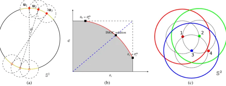
Fig. 1. Sketch map of IMOC. (a) demonstrates MOC algorithm 2 for P-C-S in S1, where u1, u2 and u3 are selected one by one with a
givenθ, and the yellow arc denotes the total coverage set. Figures (b) and (c) are sketch maps for the multi-shell case P-C-M. (b) shows the
compromise between the covering radiusθ0 in the combined shell and the covering radiusθs in thes-th shell, and demonstrates the binary
search path (the dashed blue line segment) and the obtained covering radii in IMOC. The grey area contains all feasible covering radii, and the red curve denotes all Pareto optimal covering radii. (c) demonstrates MOC for 3 shell case. Three colors denote three shells. The
numbers near the points are the selection orders in MOC for the points. Point 1 (i.e.,u1,1) is first selected for shell 1, then point 2 (u2,1) for
shell 2 and point 3 (u3,1) for shell 3. The red circle aroundu1,1 denotes its coverage setC(u1,1, θ1) which is added to CS1, and the dashed
black circle aroundu1,1 denotesC(u1,1, θ0) which is added to CS0. Point 4 (u1,2) is selected based on CSs,∀s=0,1,2,3.
find K points using θ, then θ can be decreased. Therefore, IMOC performs a binary search of the covering radiusθfrom (0, θub(2K)), where θub(2K) in Eq. (6) is an upper bound of the covering radius with K points with antipodal symmetry consideration (i.e., total 2K points) [33].
θub(2K)=arccos
s
4−csc2 πK 6(K−1)
!
(6)
See Fig. 1 (a) for a demonstration of MOC when solving P-C-S in S1 in the 2D case. It is obvious that IMOC yields the
globally optimal solutioninS1, while ISC and IGEEM cannot.
IMOC and MOC algorithms for multiple shell sampling scheme design are shown in Alg. 3 and 4. For multiple shell case, IMOC needs to search (θ0, θ1, . . . , θS) in S +1
dimensional space, where θ0 is the covering radius of the combined shell with all samples andθs(s>0) is the covering
radius of the s-th shell. There is a compromise between θ0 and θs (s > 0). The cost function in Eq. (5) essentially
converts a multi-objective optimization problem into a single objective optimization using a weighted summation. There are infinite Pareto optimal covering radii to the multi-objective optimization problem. IMOC only searches the covering radii in one dimensional space determined by the upper bounds {θub
s }Ss=0, which in practice provides good covering radii for both individual shells and the combined shell. See Alg. 3 and Fig. 1 (b) and (c). MOC in Alg. 4 first selects one point us,1
for each shell. Then it selects the best shellsand the best point
us,i whose coverage setC(us,i, θs) has the largest overlap area
with the existing total coverage set CSs∪CS0among all shells
and all candidate points outside the existing total coverage set. Similarly with ISC, for P-C, IMOC can analytically select the best point in each iteration in 2D case inS1. See Fig. 1 (a).
However, in S2, IMOC requires a fine uniform discretization of the sphere to find the best point in each step with the largest overlap area by counting the number of points in overlaping sets. For efficient implementation of IMOC, we consider 3 issues. 1) KD-tree is used for efficient nearest neighbor search. 2) The overlap area As(x) for a candidate
point x in the s-th shell can be stored for next step. In the i+1-th step, As(x) is different from the i-th step and
needs to be re-calculated, only if the determined point us0,i
in the i-th step satisfies arccos(|xTu
s0,i|) < θ0, if s , s0, or
arccos(|xTu
s0,i|) < θs, if s = s0. 3) In MOC, for P-C, the
candidate points are selected from a small“outside surface”
of CS, i.e.,{x|x<CS,∃y∈CS,s.t. arccos(|xTy|)≤δ}, instead
of the entire complementary set (S2−CS).δis set as twice of the covering radius of the fine uniform sampling set used in IMOC. It is obvious that in the 2D case, this modification does not change the result because the point in each step of MOC is always in the“outside surface”. See Fig. 1 (a). For P-C-S and P-C-M inS2, the results by IMOC do not change neither in our experiments, although we cannot give a proof. These three issues significantly speed up MOC, because the first one reduces the time for each neighborhood search, and the other two largely reduce the number of neighborhood searches. In our implementation, IMOC only requires a few seconds on an ordinary laptop.
C. 1-Opt Algorithm
We propose a greedy algorithm called 1-Opt. For both P-C and P-D, with a given initialization scheme, the 1-Opt algorithm at each step finds the best point pair (us,i from
current result andx ∈D) such that after setting us,i as x the
Algorithm 4: MOC for Multiple shell Scheme Design:
Input:{θs}Ss=0,{Ks}Ss=1,D
Output: IsSatisfied, {us,i}iK=s1.
Initialize coverage sets {CSs}Ss=0 as S +1 empty sets, and
initialize Ns=0, ∀s∈[1,S]; forn=1to PSs=1Ks do
if n==1 then choose any point asu1,1,s←1,
i←1;
if 1<n≤S then s←n,i←1, chooseus,i in
(D−CS0) such that the setC(us,i, θ0)∩CS0 has the
largest area ;
if n>S then
Set V as an empty set;
for s0=1 toS do
if Ns0<Ks0 and(D−(CSs0∪CS0))is not
emptythen
choose vs0 in (D−(CSs0∪CS0)) such that
the overlap setC(vs0, θs0)∩(CSs0∪CS0)
has the largest area denoted as As0 ; V ←V∪ {vs0};
end end
if V is emptythen
IsSatisfied =False; return else
choose sandvs∈V such that their
corresponding area As is the largest one
among{As0}S
s0=1; i←Ns+1, us,i←vs; end
end
CSs←CSs∪C(us,i, θs); CS0←CS0∪C(us,i, θ0);
Ns←Ns+1;
end
IsSatisfied=True;return;
case, 1-Opt is to increasedidefined in Eq. (2). For multi-shell
case, 1-Opt is to increase both covering radii ofus,iin the
com-bined shell, i.e., ds,i = arg max(s,i),(s0,j),∀j,∀s0arccos|usT,ius0,j0|
and in the s-th shell, i.e., di = arg maxj,i,∀jarccos|uTs,ius,j|.
See Alg. 5. 1-Opt is to increase the covering radius for every individual sample. 1-Opt requires an initialization, and a good initialization normally results in a good result. In practice, we use the result by IMOC as the initialization of 1-Opt.
Note that if IMOC is used to design a scheme with many samples for P-C, then there sometimes is a hole area in the result of IMOC. This is because of the discretization used in IMOC for P-C. By applying 1-Opt to the IMOC result, even though 1-Opt sometimes cannot increase the overall covering radius for the whole scheme, it can better arrange the points to fix the hole. See Fig. 3.
D. Constrained Non-Linear Optimization (CNLO)
For P-C, SC problem in Eq. (4) can be converted into a continuous optimization, called Constrained Non-Linear
Algorithm 5: 1-Opt for Multi-Shell Scheme Design:
Input: Initialization{u0
s,i}, and domainD Output: {us,i}.
us,i=u0s,i,∀s,i; repeat
1) Find a point pair, where one pointus,i∈ {us0,i0}and
one pointx∈D, such that after settingus,i asx,ds,i
anddi both increase (or one increases, one does not
decrease), and there is no other pair can obtain both largerds,i and larger di;
2) Setus,i tox, and removex fromD;
untilCannot find such point pair;
Optimization (CNLO):
max θ,{ui}Ki=1
θ (7a)
s.t. arccos(|uTiuj|)≥θ, ∀i< j≤K; (7b)
uTiui=1, ∀i; (7c)
where Eq. (7b) means all separation angles are larger than
θ, and Eq. (7c) means the estimated samples are on the unit sphere. After the problem is solved, the solution θ∗ is the estimated covering radius and there exists i and j such that arccos|(u∗i)Tu∗j| = θ∗. Note that both cost function and constraints are continuous.
CNLO in Eq. (7) has total K(K2−1) inequality constraints. Thus for P-C-S or P-C-M with a large number of samples, CNLO may be very slow due to large number of constraints. CNLO is a local optimization method which requires an initialization. Thus for a given initialization{pi}we propose a sped up version of CNLO to reduce the number of inequality constraints via
max θ,{ui}Ki=1
θ (8a)
s.t. arccos(|uTiuj|)≥θ, if|pTipj| ≥cos(2δ0+θub), ∀i< j≤K; (8b)
arccos(|uTipi|)≤δ0, ∀i; (8c)
uTiui=1, ∀i; (8d)
whereδ0 controls the difference between the final results{ui}
and the initialization{pi}, and the inequality constraints which have two initialization points far from 2δ0+θub do not need to be considered in Eq. (8b), because θub is an upper bound. If
δ0=0, then the result is just the initialization. Ifδ0=π/2, then the result of Eq. (8) is the same as the result of Eq. (7). When settingδ0 as a small float number, the number of constraints can be largely reduced and CNLO can be sped up.
Similarly, with a given initialization{ps,i}, P-C-M in Eq. (5) can be solved using CNLO in Eq. (9):
max
{θs},θ0,{us,i}
w1
S
S X
i=1
θs+(1−w)θ0 (9a)
s.t. arccos(|uTs,ius,j|)≥θs, if|pTs,ips,j| ≥cos(2δ0+θubs ),
∀s, ∀i< j≤Ks; (9b)
arccos(|uTs,ius0,j|)≥θ0, if|pT
∀s<s0, ∀i≤Ks, ∀j≤Ks0; (9c)
arccos(|uTs,ips,i|)≤δ0, ∀s,∀i; (9d)
θs≥θ0, ∀s; (9e)
uTs,ius,i=1, ∀s,i; (9f)
δ0 controls the difference between the result and the initializa-tion. Eq. (9b) means that the separation angles of samples in the s-th shell are larger than its corresponding covering radius
θs. Eq. (9c) means that the separation angles of samples in
two different shells are larger than the covering radius θ0 for the combined shell with all samples. Eq. (9e) means that the covering radii for all single shells are always larger than the covering radius for the combined shell, in other words, Eq. (9e) means that the separation angles of samples in the same shell are larger than θ0.
CNLO in Eq. (8) and Eq. (9) are continuous non-convex constrained optimization problems. We use sequential quadratic programming (SQP) to solve CNLO. In each step, SQP solves a quadratic programming problem which locally approximates the original non-linear problem. In practice, we use the SQP solver implemented in NLOPT library [41] (NLOPT LD SLSQP). CNLO yields a locally optimal solution with a given initialization. We suggest to use the result by IMOC + 1-Opt as the initialization. In practice, we setδ0 = 0.1, and keep performing CNLO by updating the initialization {pi} (or{ps,i}) using the previously obtained result.
E. Mixed Integer Linear Programming (MILP)
We propose a Mixed Integer Linear Programming (MILP) algorithm to solve P-D. ForD={un}nN=1, Eq. (4) can be solved
using MILP:
max θ,{hi}N
i=1
θ (10a)
s.t. arccos(|uTiuj|)≥θ−(2−hi−hj)M, ∀i> j (10b)
θlb≤θ≤θub(2K) (10c)
N X
i=1
hi=K; hi=0,1, ∀i (10d)
wherehi=1 means thatui is selected as one of theK points, θlb is a lower bound of the covering radius, which can be set to 0 or the covering radius from an existing sampling scheme,
θub(2K) is an upper bound of the covering radius in Eq. (6), andMis the difference between the maximal distance (denoted asdmax) and the minimal distance (denoted asdmin) of any two pointsui,uj∈D,i, j. After solving MILP, the solution of θ,
denoted asθ∗, is the covering radius of the selectedKsamples.
The constraint in Eq. (10b) only takes effect when two points are both selected, i.e., hi = hj = 1, and is automatically
satisfied when hi = 0 or hj = 0, because we set M large
enough such that arccos(|uTiuj|)≥dmin≥θ∗−(2−hi−hj)M,
when hi+hj≤1.
Similarly, Eq. (5) withD={us,i}can be solved using MILP:
max
{θs},{hs,i}
wS−1 S X
s=1
θs+(1−w)θ0 (11a)
s.t. arccos(|uTiuj|)≥θs−(2−hs,i−hs,j)M, ∀s,i>j (11b) arccos(|uTiuj|)≥θ0−(2−hs,i−hs0,j)M, ∀s,s0,i>j (11c)
θlb
s ≤θs≤θub(2Ks), ∀s; θ0lb≤θ0≤θub(2
S X
s=1
Ks) (11d)
N X
i=1
hs,i=Ks, ∀s; S X
s=1
hs,i≤1, ∀i; hs,i=0,1, ∀i,s (11e)
where hs,i = 1 means that ui is selected as one of the Ks
points on the s-th shell, θlbs and θub(2Ks) are the lower and
upper bounds of the covering radius on the s-th shell, and
θlb 0 and θ
ub(2PS
i=1Ks) are the lower and upper bounds for
the combined shell with all points. Similarly with Eq. (10b), constraints in Eq. (11b) and Eq. (11c) are respectively for the first and second terms in Eq. (11a). PSs=1hs,i ≤ 1 makes ui
to be selected at most in one shell such that the estimated samples are staggered across shells. Note that the above MILP in Eq. (11) is for P-D-MS. For P-D-MM, Eq. (11b) and Eq. (11c) need to be replaced by Eq. (12a) and Eq. (12b)
arccos(|uT
s,ius,j|)≥θs−(2−hs,i−hs,j)M, ∀s,i> j (12a)
arccos(|uTs,ius0,j|)≥θ0−(2−hs,i−hs0,j)M, ∀s,s0,i>j (12b)
wherehs,i=1 meansus,iis selected as one of theKspoints on
thes-th shell, andPSs=1hs,i≤1 can be removed from Eq. (11e).
Note that although in general the MILP is NP hard, it can be solved with a globally optimal solutionusing branch and bound method which iteratively solves the relaxed LP pro-gram. In our implementation, we solve Eq. (10) and Eq. (11) using GUROBI [42], which can yield the globally optimal solution or at least a reasonable solution within 10 minutes for P-D. In practice, we progressively increase the lower bound
θlb based on the solutions estimated in previous iterations to find a better feasible solution within 10 minutes which is good enough in experiments.
IV. Experiments
A. Effect of Discretization in Incremental Greedy Methods
Incremental greedy methods (i.e., IEEM [39], IGEEM [18], ISC, and IMOC), all require a uniform sample set as a discretization ofS2to determine the best sample in each step. It is obvious that a finer uniform set may not yield better results for ISC in 2D case. We test the discretization effect in S2 for both single shell and multi-shell scheme design. We consider two uniform sample sets respectively with 81 samples and 20482 samples from spherical tessellation. With
these two uniform sets, IEEM, ISC, IMOC, and IMOC +
1-Opt are performed to generate single shell scheme with
shell schemes using EEM collected in CAMINO [25]. When
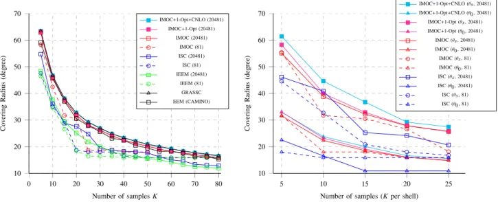
K ∈ [50,80] is close to 81 (the number of uniform samples in the coarse uniform set), covering radii by IEEM and ISC are not improved using the finer set, and when K < 50 is far from 81, IEEM and ISC obtain larger covering radii using finer discretization. When using the finer uniform set, covering radii by IMOC and IMOC + 1-Opt are improved, close to the best known solutions in GRASSC, and are much larger than covering radii of the schemes in CAMINO. ISC, IMOC, IMOC + 1-Opt are performed to generate schemes with 3 shells, K ∈[5,25] per shell by using these two uniform sets. The right subfigure of Fig. 2 shows mean of covering radii of three shells and the covering radii of the combined shell. It also demonstrates that whenK×3 is close to 81, covering radii of the combined shell by ISC are not improved using the finer set, while IMOC has no such issue. The experiment shows that IMOC and IMOC+1-Opt generally obtain better results than ISC and IEEM for P-C. CNLO can further improve the results by IMOC +1-Opt, and the covering radii by IMOC+1-Opt +CNLO obtains the best results, very closed to the solutions in GRASSC in single shell case. Thus, as shown in Table II,
ISC is suggested for P-O, and IMOC + 1-Opt + CNLO is
suggested for P-C.
B. Covering Radii in Sampling Schemes
We evaluate the proposed method by generating multi-shell schemes with K×3 samples. We test two cases withK=28 and K =90, considering these two cases were also used for evaluation in [18], and the multi-shell scheme with 90×3 samples by IGEEM was also used in HCP [18], [26].
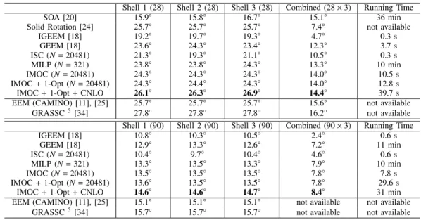
Table III shows the covering radii of the schemes by diff
er-ent methods, where IMOC + 1-Opt +CNLO means CNLO
using the result by IMOC+1-Opt as the initialization. Sparse and Optimal Acquisition (SOA) in [20], which separates a uniform scheme into several sets by using a greedy algorithm, is performed using the software released by the author 6. The result by SOA for the scheme with 90×3 samples is not shown, because it did not terminate after running for 2 days. The solid rotation method in [24] starts from the single shell scheme with 28 samples by EEM, and finds the optimal three rotations for the 3 shells, such that the electrostatic energy in the combined shell is minimized. The scheme by the solid rotation method is the 3 rotated EEM schemes, and the covering radii of the scheme were extracted from [18]. Note that we run GEEM by using the latest software released by the authors7, which obtains better covering radii for individual shells but a slightly worse covering radius for the combined shell than the original results shown in [18]. As references, the table also lists the best known results for single shell with K
andK×3 samples using EEM from CAMINO [25] and the SC formulation from 5 [34]. Note that the precomputed schemes by EEM and GRASSC are only for the single shell case, not for the multi-shell case. If this single shell scheme (with 28 or 90 samples) is repeated for 3 shells (i.e., with 3 different b values), then the covering radius for the combined shell (with
6https://sites.google.com/site/hispeedpackets/Home/soa-design 7https://github.com/ecaruyer/qspace
84 samples or 270 samples) is actually 0◦. The scheme with 84 samples by EEM is not related with the scheme with 28 samples by EEM. IMOC obtains better covering radii than incremental methods, i.e., IGEEM, ISC, and it is even better than MILP, which is because the globally optimal schemes by MILP are determined only from a coarse uniform set with 321 samples, not from a fine uniform set. It is impractical for MILP to work with 20481 samples, because MILP is NP hard. For both 28×3 and 90×3 cases, IMOC+1-Opt+CNLO obtains best schemes with largest covering radii in both 3 individual shells and the combined shell, and the covering radii by IMOC +1-Opt +CNLO in these 3 shells are even better than best known scheme collected in CAMINO using EEM [11], [25], similarly with the left subfigure in Fig. 2.
Table III also shows the running time for different methods on an ordinary laptop. Incremental methods (IGEEM, ISC, IMOC) are all very fast. IGEEM and ISC have similar running time, because they can be implemented in the same efficient way to maintain the table of increased cost functions between the selected sample set and each unselected sample, and update the table when each new sample is selected. A similar accel-eration strategy can be used for 1-Opt. MILP is terminated after 10 minutes, because we found that the cost function of MILP changes very slow after 10 minutes. Compared with the 28×3 scheme, the running time of estimating the 90×3 scheme by all methods except IMOC increases largely. The running time of GEEM increases from 3.7 seconds to 11 minites, and the running time of CNLO increases from 39.7 seconds to 31 minutes, because of the larger number of constraints. The running time of IMOC decreases for the 90×3 scheme, probably because the iteration number of MOC decreases for the 90×3 scheme, compared with the 28×3 scheme. It should be noted that the running time of scheme design methods is actually not very important for practical usage, because the schemes are optimized only once for scanners.
Fig. 3 shows the schemes by IMOC, IMOC + 1-Opt, and
IMOC + 1-Opt + CNLO. It shows that 1) IMOC + 1-Opt
can fix the hole in the scheme by IMOC; 2) IMOC +1-Opt increases the covering radii of individual shells of the scheme by IMOC, although the covering radius of the combined shell keeps the same (7.78◦); 3) CNLO can refine the scheme by IMOC+1-Opt. Thus for P-C, we do not use IMOC as a stand-alone method. Instead, IMOC+1-Opt+CNLO is suggested for P-C, where two greedy methods (i.e., IMOC+1-Opt) are used to set initialization of gradient based optimization method CNLO.
C. Rotational Invariance in Reconstruction
We test rotational invariance of the schemes with 28×3 samples by different methods in Table III. We generate syn-thetic diffusion signal from a mixture of cylinder model [43], where two cylinders cross with 60◦ and share the cylinder
0 10 20 30 40 50 60 70 80 10
20 30 40 50 60 70
Number of samplesK
Co
v
ering
Radius
(de
gree)
IMOC+1-Opt+CNLO (20481) IMOC+1-Opt (20481)
IMOC (20481) IMOC (81) ISC (20481) ISC (81) IEEM (20481)
IEEM (81) GRASSC EEM (CAMINO)
5 10 15 20 25
10 20 30 40 50 60 70
Number of samples (Kper shell)
Co
v
ering
Radius
(de
gree)
IMOC+1-Opt+CNLO (θs, 20481) IMOC+1-Opt+CNLO (θ0 , 20481) IMOC+1-Opt (θs, 20481) IMOC+1-Opt (θ0 , 20481) IMOC (θs, 20481) IMOC (θ0 , 20481)
IMOC (θs, 81) IMOC (θ0 , 81) ISC (θs, 20481) ISC (θ0 , 20481)
ISC (θs, 81) ISC (θ0 , 81)
Fig. 2. Effect of discretization. The left figure shows the covering radii of single shell schemes withKsamples obtained by methods using
two uniform sets with 81 samples and 20481 samples. The right figure shows the covering radii of multi-shell schemes with K×3 samples,
whereθs is the mean of covering radii in three shells, andθ0 is the covering radius of the combined shell.
IMOC IMOC +1-Opt IMOC+1-Opt+CNLO
(13.49◦, 13.48◦, 13.49◦, 7.78◦) (13.56◦, 13.50◦, 13.50◦, 7.78◦) (14.56◦
, 14.64◦, 14.69◦,8.40◦)
Fig. 3. Multi-shell sampling schemes with 90×3 samples generated by three methods, and the covering radii of 3 shells and the combined shell in schemes shown in Table III. The colors differentiate the sampling points from the three shells. Note that there is a hole area in the scheme by IMOC, which can be fixed by 1-Opt and CNLO.
Deconvolution (NNSD) [9] with the spherical harmonic (SH) order 8 to estimate fODFs, detect the peaks, and calculate the mean angular differences by comparing the detected peaks with the ground-truth fiber directions in these 20481 tests. A good sampling scheme should give low mean angular differences with low standard deviations. Table IV lists the mean and standard deviation of angular differences obtained
by NNSD using different schemes. IMOC + 1-Opt +CNLO
yields the lowest angular differences with the lowest deviation, and IMOC has the lower mean and deviation than IGEEM.
We compare the 28×3 schemes and 90×3 schemes in DWI signal reconstruction by using tensorial Spherical Polar Fourier Imaging (SPFI) [16]. The DWI signals are synthesized using a mixture of tensor model with two symmetric tensors with eigenvalues [1.7,0.2,0.2]×10−3mm2/s with a crossing angle of 60◦. We rotate the model and generate signals 20481 times with the rotation angles determined by the uniform sample set with 20481 samples. Tensorial SPFI with spherical order of 8
and radial order of 4 is used to fit the data and re-sample the DWI signals at continues 3 shells with a fine tessellation of 20481 samples. Then normalized mean Root-Mean-Squared-Error (RMSE) of DWI signals in 3 shells is calculated. We also add Rician noise with SNR=30 (i.e., standard deviation of 1/30) for 1000 trails, and re-calculate mean normalized RMSE in reconstruction using noisy samples. Table V shows the mean and standard deviation of normalized RMSE in reconstruction using noise-free samples and noisy samples. It shows that
IMOC + 1-Opt + CNLO obtains lower mean and std of
TABLE III
Covering radii of multi-shell sampling schemes with28×3and90×3samples generated by various methods with the corresponding running time.
Shell 1 (28) Shell 2 (28) Shell 3 (28) Combined (28×3) Running Time
SOA [20] 15.9◦ 15.8◦ 16.7◦ 15.1◦ 36 min
Solid Rotation [24] 25.7◦ 25.7◦ 25.7◦ 7.4◦ not available
IGEEM [18] 19.2◦ 19.7◦ 19.3◦ 4.7◦ 0.3 s
GEEM [18] 23.6◦ 24.3◦ 23.4◦ 12.3◦ 3.7 s
ISC (N=20481) 21.3◦ 19.3◦ 21.1◦ 10.5◦ 0.3 s
MILP (N=321) 23.8◦ 23.8◦ 24.3◦ 13.3◦ 10 min
IMOC (N=20481) 24.3◦ 24.3◦ 24.3◦ 14.0◦ 10.5 s
IMOC+1-Opt (N=20481) 24.3◦ 24.4◦ 24.3◦ 14.0◦ 12.8 s
IMOC+1-Opt+CNLO 26.1◦ 26.3◦ 26.9◦ 14.4◦ 39.7 s
EEM (CAMINO) [11], [25] 25.7◦ 25.7◦ 25.7◦ 15.6◦ not available
GRASSC5[34] 27.8◦ 27.8◦ 27.8◦ 16.2◦ not available
Shell 1 (90) Shell 2 (90) Shell 3 (90) Combined (90×3) Running Time
IGEEM [18] 10.8◦ 10.3◦ 10.5◦ 2.4◦ 0.6 s
GEEM [18] 12.9◦ 13.3◦ 12.6◦ 7.2◦ 11 min
ISC (N=20481) 10.4◦ 9.7◦ 10.4◦ 4.6◦ 0.6 s
MILP (N=321) 13.3◦ 13.5◦ 13.3◦ 7.9◦ 10 min
IMOC (N=20481) 13.5◦ 13.5◦ 13.5◦ 7.8◦ 7.8 s
IMOC+1-Opt (N=20481) 13.6◦ 13.5◦ 13.5◦ 7.8◦ 29.6 s
IMOC+1-Opt+CNLO 14.6◦ 14.6◦ 14.7◦ 8.4◦ 31 min
EEM (CAMINO) [11], [25] 15.1◦ 15.1◦ 15.1◦ not available not available
GRASSC5[34] 15.7◦ 15.7◦ 15.7◦ not available not available
the hole area effect in IMOC. IMOC + 1-Opt and IMOC + 1-Opt +CNLO reduce the rotational invariance of IMOC.
D. MILP for Separation of Sampling Schemes
We evaluate the effectiveness of the proposed MILP in Eq. (11) withw=1 to solve P-D-MS, by verifying whether it can separate a set of samples into several subsets, keeping the points in each subset as uniform as possible. We compared
MILP with the subsetpoints program in CAMINO [11],
[25] and dirsplit in MRtrix 8 for the same task. For this evaluation, we randomly mix two sets of uniform points, where one set has 81 points generated by spherical tessellation (with covering radius 15.9◦) and the other set has 60 points (with
covering radius 18.3◦) from CAMINO generated by EEM. Separation of these 141 points into subsets respectively with 81 and 60 samples should ideally give results that match the original uniform point sets. MILP obtained results that exactly match the original point sets within 1 second.subsetpoints
in CAMINO, which minimizes electrostatic energy by using simulated annealing, saves the result every hour when it runs. It obtains two incorrect points in each subset after running for 2 hours, 7 incorrect points after 8 hours, and the correct result after 9 hours. Although the correct result has been obtained, the program continues to run for hours until the simulated annealing temperature is finally small enough. dirsplit in MRtrix initializes two sets and then randomly swaps 2 direc-tions in each step to reduce the electrostatic energy.dirsplit
can only separate the scheme into 2 schemes with nearly equal numbers 71 and 70. With default parameters and multi-threading, it finished running after 16 minutes. However, the covering radii in these two sets are 6.4◦ and 5.1◦ respectively, different from the original two uniform sets.
E. MILP for sub-sampling of multi-shell HCP scheme
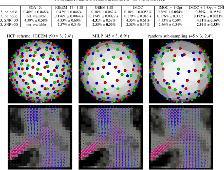
In order to reduce the scanning time and reuse the existing data, we may want to uniformly select a sub-sampled scheme from an existing scheme. IGEEM has been successfully used in multi-shell diffusion data acquisition in HCP [17], [18], [26]. The scheme has 3 shells with b values 1000, 2000, and 3000 s/mm2, 90 samples per shell. See top left subfigure in Fig. 4. MILP and a random selection are performed to obtain two sub-sampled schemes with 45×3 samples. It is a problem of P-D-MM, which to our knowledge can not be solved by any existing released routine (e.g., in CAMINO or MRtrix). MILP yields the covering radius 7.0◦ in the combined shell, while
the random selection yields 2.4◦, which is the same as the
original HCP scheme. See first row in Fig. 4. We also perform NNSD with SH order 8 on a subject with the full scheme of 90×3 samples and two sub-sampled schemes with 45×3 samples from MILP and random selection. The corresponding fODF fields with detected peaks are displayed in Fig. 4 with GFA as backgrounds. Peaks are detected from the fODFs with GFA higher than 0.5. Fig. 4 shows that the estimated fODF and peaks from sub-sampled scheme by MILP are much closer to the results from the full scheme, compared with the random selection. Note that fODFs near grey matter areas by the scheme from random selection are very noisy, compared with the results using the full scheme. That is because that random selection cannnot keep the uniformity in the sub-sampled scheme. In the region visualized in Fig. 4, the mean angular difference of the detected peaks is 4.2◦ between the
results from the full scheme and the sub-sampled scheme by MILP, and 5.9◦ between the results from the full scheme and
the sub-sampled scheme by random selection. The normalized RMSE of the estimated GFA of fODFs is 7.5% for the sub-sampled scheme by MILP and is 18.9% for the scheme by random selection.
TABLE IV
Angular differences between estimated directions and ground-truth fiber directions using different schemes by various methods.
SOA [20] IGEEM [17], [18] GEEM [18] IMOC IMOC+1-Opt IMOC+1-Opt+CNLO
Angular Difference 1.41◦±0.75◦ 1.67◦±0.81◦ 1.23◦±0.73◦ 1.43◦±0.77◦ 1.31◦±0.71◦ 1.16◦ ±0.64◦
TABLE V
NormalizedRMSEofDWIsignal reconstruction using tensorialSPFI.
SOA [20] IGEEM [17], [18] GEEM [18] IMOC IMOC+1-Opt IMOC+1-Opt+CNLO
28×3, no noise 0.46%±0.048% 0.42%±0.046% 0.38%±0.062% 0.38%±0.0058% 0.36%±0.054% 0.35%±0.055% 90×3, no noise not available 0.176%±0.0044% 0.174%±0.0022% 0.179%±0.016% 0.176%±0.0035 0.172%±0.0021% 28×3, SNR=30 4.39%±0.58% 4.33%±0.60% 4.31%±0.58% 4.35%±0.61% 4.33%±0.59% 4.31%±0.56% 90×3, SNR=30 not available 2.57%±0.34% 2.55%±0.33% 2.58%±0.35% 2.56%±0.34% 2.54%±0.33%
HCP scheme, IGEEM (90×3, 2.4◦) MILP (45×3,6.9◦
) random sub-sampling (45×3, 2.4◦)
Fig. 4. First row: full HCP scheme, sub-sampled schemes by MILP and random selection, respectively. Second row: fODFs fields estimated from the data sets corresponding to schemes, where fODF glyphs are colored by directions, the background is the GFA map, and the yellow tubes denote detected peaks.
V. Discussion
A. Sampling scheme design without antipodal symmetry
The SC formulation and EEM formulation [11], [17]–[23] both are to design sampling schemes with the antipodal sym-metry constraint, based on prior knowledge that the diffusion signal is antipodal symmetric, i.e., E(q) =E(−q). However, some works proposed to model asymmetry of diffusion sig-nals [44] or fiber ODFs [45], which may prefer sampling schemes without the antipodal symmetry constraint. Moreover general uniform single or multiple shell sampling schemes (i.e., without the antipodal symmetry constraint) are also be useful in some applications other than diffusion MRI.
Although the proposed SC formulation and 5 algorithms focus on sampling scheme design with antipodal symmetry, they can be easily performed to design general sampling schemes without the antipodal symmetry constraint. Actually the original SC formulation in mathematics [33], [35] does not consider the antipodal symmetry constraint. If the absolute
B. Sampling scheme design with other considerations
1) Diffusion models and model fitting: As discussed in
the introduction part, both the SC formulation and EEM formulation are to design uniform sampling schemes in single or multiple shells with parameters S and {Ks}Ss=1. This is
based on the fact that diffusion signals in voxels have various preferred orientations, while we need to design one scheme for all signals in human brain. The number of b values S, and the number of samples in each shell {Ks}Ss=1, are both user determined. Different diffusion models, e.g., tensor model and various HARDI models, may prefer different distributions of b values in the radial part of the q-space, and different number of samples in low or b values. Moreover, even for the same model, different model fitting algorithms may prefer different schemes [12]. The samples with high b values capture more orientational information, while have lower single-to-noise ratio (SNR), than the samples with low b values. Thus robust estimation algorithms [9], [14], [16], which are less sensitive to noise, may prefer larger number of samples with high b values.
2) Eddy current correction: Recent works on eddy
cur-rent correction [29], [46], [47] showed that three kinds of acquisitions are useful for eddy current correction, i.e., 1) the blip-up blip-down acquisition, which scans the the data twice with flipped phase-encoding directions; 2) the acquisition with gradients on the whole sphere that includes both{ui}and{−ui};
3) the acquisition with gradients on the whole sphere without the antipodal symmetry constraint. Schemes by SC can be directly used in the blip-up blip-down acquisition with flipped phase-encoding directions. and can be used in the second kind of acquisition by incorporating the flipped gradients {−ui}.
For the third acquisition on the whole sphere without the antipodal symmetry constraint, we can perform the proposed optimization methods without the constraint, as described in Section V-A.
3) Gradient reorientation: The uniform schemes generated
by SC or EEM are used to scan DWI data. Some pre-processing steps, including motion correction, eddy current correction, registration of DWIs, etc., may require gradient reorientation [48], [49]. Gradient reorientation changes each individual gradient, and also the separation angles between gradients. Thus even though the designed schemes by SC for scanning data are optimized with large angular separa-tion, the reorientated scheme for model fitting may be sub-optimal. This issue also exists for schemes by EEM, where the electrostatic energy is sub-optimal after reorientation. The gradient reorientation issue has not been considered in existing works on uniform scheme design [11], [17]–[23], because the transform matrix for each gradient vector is dependent on DWI images and also the image registration algorithm used in the preprocessing steps. In this paper, we show that in both SC and EEM formulations, uniform sampling scheme design before gradient reorientation is an approximation of uniform sampling scheme design after gradient reorientation, in an approximation algorithm point of view 9.
9https://en.wikipedia.org/wiki/Approximation algorithm
Intuitively, if the transform matrix is close to the identity matrix, then the reoriented scheme are closed to the original scheme which has been well optimized. This intuition can be quantitatively described in Proposition 1, which shows that if the transform matrix is inside a ball of the identity matrix with radiusδ, then the inner product of two reoriented gradient vectorsxT
1x2 is inside a range centered at the inner product of the original two gradient vectorsuT
1u2with a radius of 2δ+δ 2. The proof of this proposition is shown in Appendix A.
Proposition 1: Angular separation after gradient
reori-entation.Letu1 andu2 be two gradient vectors inS2. Denote the two gradient vectors after reorientation as x1 and x2, and the corresponding transform matrices asT1 andT2 such
that xi = Tiui, i = 1,2. If kTi −Ik2 ≤ δ, where I is the identity matrix, then the reoriented gradient vectors satisfies |xT
1x2−u
T
1u2| ≤2δ+δ 2.
Note that Proposition 1 works for gradient reorientation using rotation matrices and also general affine transforms [48], where if Ai is the affine matrix used to reorientui such that
xi = kAAiui
iuik2, then Ti =
Ai
kAiuik2. Proposition 1 means that the separation angle of two reoriented gradients arccos(xT
1x2) is in [arccos(uT
1u2+2δ+δ
2),arccos(uT
1u2−2δ−δ
2)]. And the minimal separation angle of any two reoriented gradients is also in a range defined by the separation angle of two original gradient vectors. Thus, in an approximation algorithm point of view9, maximizing the angular separation of the original scheme for scanner is to approximately maximize the angular separation of the reorientated scheme for model fitting. In practice, the transform matrix between a reoriented gradient vector and an original gradient vector in motion correction or eddy current correction is close to the identity matrix, i.e.,kT−Ik2< δ, and
δ is a small value. If the transform matrix T is the rotation aboutz-axis with the degree of 5◦, then=0.123 that is about
12% of the norm of I. In practice, the rotation angle of the transform matrix is smaller than 5◦. Thus the change of the
separation angle after gradient reorientation is small.
For the EEM formulation, as shown in Eq. (1), the electro-static energy betweenui anduj is
f2(ui,uj)= 1 kui−ujk22
+ 1
kui+ujk22
= 1
1−(uT iuj)2
∈ 1 1−(|uT
iuj| −2δ−δ2)2
, 1
1−(|uT
iuj|+2δ+δ2)2 (13)
Based on Proposition 1, after gradient reorientation, the electrostatic energy betweenxiandxj is
f2(xi,xj)= 1 1−(xT
ixj)2 ∈ 1 1−(|uT
iuj| −2δ−δ2)2
, 1
1−(|uT
iuj|+2δ+δ2)2 (14)
Note that here we assume|uTiuj|+2δ+δ2<1. The length of
the range is
1 1−(|uT
iuj|+2δ+δ2)2
− 1
1−(|uT
iuj| −2δ−δ2)2
= 4|u
T iuj|(2δ+δ
2)
(1−(|uT
iuj|+2δ+δ2)2)(1−(|u T
iuj| −2δ−δ2)2) ≤ 4c0(2δ+δ
2)
(1−(c0+2δ+δ2)2)(1−(c0−2δ−δ2)2)=
L(c0, δ) (15)
wherec0=maxi<j|uTiuj|<1−2δ−δ2. Thus, the electrostatic
energy of the reoriented sampling schemeP
the electrostatic energy of the original scheme P
i<jf2(xi,xj),
are both inside a range, and we have
X
i<j
f2(ui,uj)− X
i<j
f2(xi,xj)
≤K(K−1)L(c0, δ) (16)
whereK is the number of samples in the single shell scheme. Thus, minimizing the electrostatic energy of the original scheme is to approximately minimize the energy of the re-oriented scheme. When δ is small, i.e., the transform matrix is close to the identity matrix, the range length in Eq. (16) is small and the electrostatic energies of the original scheme and the reoriented scheme are close.
We have shown that uniform sampling scheme design before gradient reorientation is an approximation of uniform sampling scheme design after gradient reorientation. However, it should be noted that if the transform matrix due to gradient reorientation is far from the identity matrix, the approximation error can be large. As shown in experiments, the proposed SC method yields larger angular separation (i.e., covering radius) between samples than the state-of-the-art EEM and GEEM method. If we assume that gradient reorientation reduces the covering radius of all schemes by the same amount (< 5◦), then, after gradient reorientation, the scheme by SC still has larger covering radius than the scheme by EEM.
4) Minimizing gradient heating: The SC formulation in
this paper is to design uniform sampling scheme in shells, similarly with the works based on EEM [11], [17]–[23], which have not yet considered gradient heating specifically. We have proposed to use ISC for P-O, where the first partial set of samples are nearly uniformly separated. It was reported in [40] that optimal ordering not only ensures that usable data are available if the scan needs to be cut short, but also reduces the risk of systematic errors due to gradient heating and subject motion. Minimizing gradient heating is beyond of the content of this paper, and gradient heating may be reduced in different ways [50], [51]. It can be a future work to investigate which way of reducing gradient heating is more appropriate to be incorporated into current SC framework in this paper.
VI. Conclusion
In this paper, we proposed to use the Spherical Code con-cept, which directly maximizes angular separations between samples, to design single- and multi-shell uniform sampling schemes. We showed that various continuous and discrete sampling scheme design problems can be formulated using SC. We proposed five novel algorithms (i.e., ISC, IMOC, 1-Opt, MILP, CNLO) based on SC for uniform sampling scheme design. See Table I. ISC is mainly to order samples in an exist-ing scheme. IMOC and 1-Opt are to quickly obtain schemes in deterministic greedy ways. Although IMOC is a greedy incremental method, it obtains globally optimal solution in
S1. For the sphereS2 in dMRI, covering radii of schemes by IMOC are very close to the best known solutions in single shell case5, and are much larger than EEM in CAMINO. CNLO is a local optimization method which refines a given initialization (normally from IMOC+1-Opt). MILP is used to perform sub-sampling in an existing scheme. It can obtain globally
optimal solution or a good result within 10 minutes. The experiments showed that compared with the state-of-the-art methods [18], [20] based on electrostatic energy which is used in HCP, the multi-shell scheme by IMOC +1-Opt +CNLO yields larger covering radii in general, and better rotational invariance in dMRI reconstruction when the SNR is high and the number of samples is small. However, when a large number of noisy samples are used in DWI reconstruction, the sampling schemes by different methods may have similar reconstruction results. The proposed SC methods are to maximize the angular separation between samples, independent of diffusion models and diffusion reconstruction. The optimal sampling scheme that yields the best reconstruction quality is dependent on the diffusion model, reconstruction algorithm, and the ground truth diffusion signal. It is a future work to optimize the sampling schemes for a given specific diffusion model and a given reconstruction algorithm, so that the final result of the diffusion reconstruction is optimized. We have released some demos and codes in DMRITool1.
AppendixA Proof ofProposition1
DenoteTi=I+Ci, then we have kCik2≤δ, and xT1x2=uT1(I+C
T
1)(I+C2)u2 =uT1u2+uT1(C
T
1 +C2)u2+uT1C
T
1C2u2 Letc=|uT1(CT1 +C2)u2|+|uT1CT1C2u2|, then
|xT
1x2−uT1u2| ≤c
Because|uT1(CT1+C2)u2| ≤ kCT1+C2k2 ≤2δ, and|uT1CT1C2u2| ≤ kCT
1k2kC2k2=δ
2, we havec≤2δ+δ2. Then |xT
1x2−uT1u2| ≤2δ+δ2 (17) Acknowledgments
The authors would like to thank Dr. Ruiliang Bai and Dr. Alexandru Avram for useful discussions. This work was supported in part by funds provided by the Intramural Re-search Program of theEunice Kennedy ShriverNational Insti-tute of Child Health and Human Development (NICHD) (ZIA-HD000266), and NIH grants (NS093842 and EB022880). The data were provided in part by the Human Connectome Project, WU-Minn Consortium (Principal Investigators: David Van Essen and Kamil Ugurbil; 1U54MH091657) funded by the 16 NIH Institutes and Centers that support the NIH Blueprint for Neuroscience Research; and by the McDonnell Center for Systems Neuroscience at Washington University.
References
[1] P. J. Basser, J. Mattiello, and D. LeBihan, “MR Diffusion Tensor Spectroscropy and Imaging,”Biophysical Journal, vol. 66, pp. 259–267, 1994.
[2] D. S. Tuch, T. G. Reese, M. R. Wiegell, N. Makris, J. W. Belliveau, and V. J. Wedeen, “High Angular Resolution Diffusion Imaging Reveals Intravoxel White Matter Fiber Heterogeneity,”Magnetic Resonance in Medicine, vol. 48, pp. 577–582, 2002.