Index Catalog // Carolina Digital Repository

(1)

New Approaches to Discrete Choice and Time-Series

Cross-Section Methodology for Political Research

by

Jonathan Kropko

A dissertation submitted to the faculty of the University of North Carolina at Chapel Hill in partial fulfillment of the requirements for the degree of Doctor of Philosophy in the Department of Political Science.

Chapel Hill 2011

Approved by:

George Rabinowitz, Advisor

John Aldrich, Committee Member

Thomas Carsey, Committee Member

Skyler Cranmer, Committee Member

(2)

c

2011

(3)

Abstract

JONATHAN KROPKO: New Approaches to Discrete Choice and Time-Series Cross-Section Methodology for Political Research.

(Under the direction of George Rabinowitz.)

(4)

(5)

(6)

Acknowledgments

I would especially like to thank George Rabinowitz for all of his help and guidance. As my advisor, he pushed me to the point where I could see the finish line, but he was not able to cross it with me. If the research contained in this dissertation is in any way impressive, much of the credit belongs to George. If the research is unimpressive, the credit is mine.

This dissertation would not have been possible without the support of family and friends: Marv and Olga Kropko, Josh Kropko, Tia Kropko, Tamara Mittman, Jessica Brandes, Emanuel Coman, Ian Conlon, Shaina Korman-Houston, Caitlin LeCroy, Rachel Meyerson, Zach Robbins, Samantha Snow, and Sarah Turner.

I owe a great deal to the consultants at the Odum Institute for Research in the Social Sciences: Augustus Anderson, Ryan Bakker, Kimberly Coffey, Tab Combs, Anne K. Hunter, Heather Krull, Gerald Lackey, James E. Monogan, Evan Parker-Stephen, Jessica Pearlman, Daniel Serrano, Brian Stucky, Chris Wiesen, Bev Wilson, and Cathy Zimmer.

(7)

List of Figures

2.1 Within Effects, the Between Effect of Case-Level Averages, and the Overall OLS Effect. . . 34

2.2 OLS Coefficient Point Estimates for GDP Per Capita, with 95% Confi-dence Intervals, From 1950 to 2006 . . . 50

2.3 An Example of How to Calculate the “Updated”N for OLS Results in 1952. 54

2.4 Between Effect Coefficient Estimates, From 1950 to 2006 . . . 63

2.5 OLS and BEER Estimates of the Between Effect of Median State Income. 67

2.6 OLS and BEER Estimates of the Between Effect of Median State Income and Updated Sample Sizes. . . 69

2.7 The “True” Between Effects Generated by Each Data Generation Model. 77

(12)

List of Tables

1.1 Example Discrete Choice Data. . . 12

1.2 Correlations Between Coefficient Estimates from MNL, MXL, and MNP and the True Coefficients. . . 21

1.3 Percent Correct Signs of Coefficient Estimates from MNL, MXL, and MNP. 21

1.4 Evaluation Statistics for the Three Estimators, Increasing the Number of Draws. . . 23

1.5 Percent Correct Inferences on Coefficient Estimates from MNL, MXL, and MNP. . . 25

1.6 Failure Rates and Average Time to Successfully Converge for MNL, MXL, and MNP. . . 26

1.7 Errors in Predicted Probabilities from MNL, MXL, and MNP. . . 28

1.8 Comparison of Parameter Estimates Which Account for Error Correlation. 30

2.1 Example of Between and Within Parts of a Variable in TSCS Data . . . 40

2.2 Countries in the Sample and Average Regional Authority Index . . . 57

2.3 Results for the Regional Authority Regression. . . 60

2.4 Groups from Average Linkage Cluster Analysis on Year Dissimilarity, Six Group Solution . . . 64

2.5 Groups from Average Linkage Cluster Analysis on Year Dissimilarity, Five Group Solution . . . 68

2.6 Simulation parameters: DGP 1. . . 75

2.7 Simulation Parameters: DGP 2 and 3. . . 76

(13)

2.9 Absolute Divergence and Coverage Percentage for Each Method Using Each of the Four Data Generating Processes. . . 83

3.1 MCMC Results for the NL-Logit Model: 1984 and 1996 . . . 100

3.2 MCMC Results for the NL-Logit Model: 2004 and 2008 . . . 101

3.3 Convergence Diagnostics for the NL-logit Model of the 1984, 1996, 2004, 2008 ANES. . . 104

3.4 Comparisons of the Moderation Effects of the Levels of Personal Importance106

A.1 Regression of Party Affect, 1987 Britain Election Study. . . 109

B.1 Basic Model Correlations Between Coefficient Estimates and the True Co-efficients, and Percent Correct Signs . . . 112

B.2 Basic Model Failure Rates. . . 112

B.3 Britain Model Failure Rates, and Correlations Between Coefficient Esti-mates and the True Coefficients. . . 113

(14)

List of Abbreviations

• ANES: American National Election Study • BE: between estimator

• BEER: the between effects estimation routine

• CDF: cumulative density function • DGP: data generating process

• DUE: decomposed unit effect • FE: fixed effects

• FEVD: fixed effects with vector decomposition

• GDP: gross domestic product

• GEE: generalized estimating equations

• GHK: Geweke-Hajivassilou-Keane algorithm

• GMM: generalized method of moments • IIA: independence of irrelevant alternatives

• LL: log-likelihood

• LOWESS: locally weighted scatterplot smoothing

• MCMC: Markov-chain Monte Carlo

• ML, MLE: maximum likelihood, maximum likelihood estimation • MNL: multinomial logit

• MNP: multinomial probit • MSE: mean squared error

• MXL: mixed logit, or random parameters logit

• NL: non-linear

• NLS: non-linear least squares

• OLS: ordinary least squares

(15)

• PDF: probability density function • RAI: regional authority index

• RE: random effects

• Reg: individual regressions for each time point • SD: standard deviation

• SDP: Social Democratic Party • SE: standard error

• TE: time effects

• TE1: time effects interacted with linear time • TE2: time effects interacted with quadratic time

(16)

Chapter 1 A Comparison of Three Discrete

Choice Estimators

1.1 Summary

(17)

1.2 Introduction

Researchers who model discrete choices, such as the choice of a voter in a multiparty election, must choose between competing empirical estimators for the model. Several estimators for discrete choice models are now easily implemented in statistical software packages, and three options available to researchers are multinomial logit (MNL), multi-nomial probit (MNP), and mixed logit (MXL) which is also called random parameters logit. Technically, these estimators are very similar: they differ only in the distribution of the error terms. MNL has errors which are independent and identically distributed, and MNP and MXL use more general distributions which allow errors to be correlated.1

The independent errors of MNL force an assumption called independence of irrelevant alternatives (IIA). Essentially, IIA requires that an individual’s evaluation of an alterna-tive relaalterna-tive to another alternaalterna-tive should not change if a third (irrelevant) alternaalterna-tive is added to or dropped from the analysis. When IIA is violated, MNL cannot produce accurate estimates of substitution patterns, which are marginal effects of covariates when an alternative is hypothetically considered to have dropped out of the analysis. MNL is an inappropriate estimator for researchers who are interested in the perceived similarity between choices, or the proclivity of individuals to substitute one alternative for another. MNP and MXL do not assume IIA: although they do not estimate the error correlations, they do estimate parameters which account for these correlations. Many researchers use MNP and MXL as better theoretical models for the data.

Most of the work to describe the problems caused by IIA focuses on the inability of MNL to estimate substitution patterns. But it is important to note that MNL incorrectly specifies a model when IIA is violated, and therefore coefficient estimates are inconsis-tent. The nature of this inconsistency is not well understood: the severity of the bias,

1_{The following abbreviations will be used frequently throughout the article: MNL refers to}

(18)

and whether the bias becomes more severe as IIA becomes a less tenable assumption, are unclear. As Dow and Endersby (2004) have previously discussed, the principle concern of researchers who must choose a discrete choice estimator is not accurate estimation of sub-stitution patterns, but rather the ability of the estimator to return accurate coefficients and inferences, and to do so reliably.

Other researchers have used MNP and MXL to produce estimates of the residual correlation between choices. However, as discussed in section 1.3.3 and as described previously by Bolduc (1999) and Keane (1992), while MNP and MXL estimate parameters to account for residual correlation, the individual correlations between residuals cannot be separately identified by MNP or MXL.

The goal of the analysis presented here is to inform the decisions of researchers in the field who must choose between MNL, MNP, and MXL. I consider the relative per-formances of the three estimators on 7 criteria: (1) the accuracy of coefficient point estimates, (2) the rate of correct signs and (3) correct inferences for coefficient estimates, (4) the frequency with which each estimator fails to converge to meaningful results, (5) the time it takes for each estimator to converge, (6) the accuracy of predicted probabili-ties, and (7) estimates of parameters to account for error correlations. The comparisons are conducted using Monte Carlo simulations.

The simulations suggest that, contrary to the focus of the literature, the validity of the IIA assumption should not be a major concern for researchers in choosing between the three estimators. The results indicate that, in most situations, MNL provides more accurate point estimates than MXL or MNP even when the IIA assumption is severely violated. If the goal is to estimate choice probabilities, then the simulations suggest that MNP provides an improvement over MNL and MXL, but at the expense of the coefficient estimates.

(19)

properties of a statistical model or estimator. “True” parameter values are specified be-forehand, and the results are analyzed in each iteration to see how accurately they return these parameter values. A comparison of discrete choice estimators, however, presents unique challenges. The binary logit and probit models differ in their specifications in that a logit model assumes a logistic distribution for the residuals and probit uses a standard normal distribution for the residuals. These distributions only vary significantly at the tails. More importantly, they assume different variances, leading to coefficient estimates which are not directly comparable to the true parameter values because of a difference in scaling. For the same reason, MNL and MNP coefficients for the same model are not directly comparable to each other.

One important challenge for this research is the development of a technique to com-pare MNL, MXL, and MNP coefficients to true parameter values and to each other in a way which removes the differences between the coefficients due to the scaling of each esti-mator. This technique is described in detail in section 1.5.1. With the scaling-differences removed, the models still differ in the functional form of their likelihood functions. MNL and MXL use a multivariate logistic link function, and MNP uses a multivariate normal distribution. In the simulations, the data are generated using a multivariate normal dis-tribution; so MNP has something of a “home field advantage.” Despite this advantage, MNL and MXL consistently outperform MNP in returning accurate coefficient point estimates.

(20)

1.3 Background

There has been a great deal of work which compares MNL and MNP on theoretical or empirical grounds, and this project builds on that work in two ways. First, since MXL is included, three well-known estimators are compared rather than two. Second, the estimators are compared on the accuracy of their coefficient point estimates. Much of the previous work on choosing between MNL and MNP focuses on whether MNL coefficients change when a candidate is added or dropped from the analysis rather than on the consistency of MNL coefficients when IIA is violated in the full choice-set.2

In political science, some comparisons have focused on the question of whether IIA is a tenable theoretical assumption for a specific election. Alvarez and Nagler (1998) and Quinn et al (1999) compare relative suitability of MNL and MNP for elections in Britain and in the Netherlands. Other comparisons have been empirical. Dow and Endersby (2004) use MNL and MNP to estimate the same models of voter choice in the 1992 U.S. presidential election and 1995 French presidential election and find little difference between predictions whether MNL or MNP is used. They argue that given the concerns of the identification of MNP discussed by Keane (1992), researchers should be more confident in the MNL results. In their 1994 paper, Alvarez and Nagler conduct simple Monte Carlo simulation experiments to demonstrate that on a number of criteria MNP outperforms models which assume IIA. They generate data with a known covariance structure in the choice errors, and alter the correlations as an experimental treatment. A similar methodology is adopted for the comparisons made in this paper.

2_{On this basis, tests for IIA violation were developed to indicate whether MNP should be used instead}

(21)

1.3.1 Statistical Framework

All three estimators model discrete choices by using the framework of a random utility model, which derives latent utilities for each individual for choosing each alternative. An individual’s choice is the alternative with the highest utility, and the probability of this choice is the probability that the associated utility is the highest among the alterna-tives. For example, a voter in the 1987 British election chose between the Conservative party, the Labour party, and the Social Democratic Party-Liberal Party alliance. For a particular voter, a random utility model uses three separate equations to estimate the voter’s evaluation of the Conservative and Labour parties and the SDP-Liberal alliance. Formally, individual i evaluates alternativej according to the equation

Uij =Vij+εij, (1.1)

where Vij represents the deterministic part of the evaluation and εij is the residual,

stochastic part of this evaluation. Vij may be modeled linearly, containing covariates

and estimated coefficients. A model which assumes that corr(εj, εk) = 0 for any two

alternatives j and k makes the IIA assumption. For all three estimators, the likelihood function for a model withN individuals choosing between J alternatives is

L=

N Y

i=1

J Y

j=1

P(yi =j)Iij, (1.2)

where Iij = 1 if individual i chooses alternative j and is 0 otherwise. MNL, MXL, and

MNP use different functions for the choice probability P(yi =j).

(22)

or MXL. For notational ease, let

η2 =ε2−ε1, and η3 =ε3−ε1. (1.3)

The probability of choosing alternative 1 is the probability that alternative 1 is the most highly evaluated, so that U1 is greater than both U2 and U3:

P(yi = 1) =P(Ui1 > Ui2 and Ui1 > Ui3)

=P(Vi1 +εi1 > Vi2+εi2 and Vi1+εi1 > Vi3 +εi3)

=P(ηi2 < Vi1−Vi2 and ηi3 < Vi1−Vi3)

=

Z Vi1−Vi2 −∞

Z Vi1−Vi3 −∞

f(η2, η3)dη3 dη2, (1.4)

wheref(η2, η3) is the joint PDF of η2 and η3. MNL, MXL, and MNP differ only in their

assumptions about this distribution. MNL uses a distribution which assumes IIA, but has an analytic integral, so that estimates are relatively easy to compute even when there are a large number of alternatives. MNL and the IIA assumption are discussed in more detail in section 1.3.2. MNP and MXL are more general than MNL, and do not assume IIA. However neither one uses choice probabilities which can be integrated analytically, so numerical methods must be used to approximate the integral in equation 1.4.3 _These

two estimators are discussed in section 1.3.3.

3_{MNP uses the Geweke-Hajivassilou-Keane (GHK) simulation algorithm for approximating}

(23)

1.3.2 MNL and the IIA Assumption

Presently, most political science articles that estimate a discrete choice model use MNL. Computation of MNL is highly efficient because the choice probability has an analytic solution:

P(yi = 1) =

eVi1

eVi1 +eVi2 +eVi3. (1.5)

This convenient form for the MNL choice probabilities depends on two assumptions. The first assumption is that error terms in equation 1.1 are distributed by the type-1 extreme value distribution. The second assumption is that the error terms are also independent, which is the IIA assumption.4

The substantive implication of IIA that is often inappropriate is that the odds ra-tio between two alternatives depends only on informara-tion about those two alternatives, and no information about any other alternative will change this ratio. In modeling a multiparty election, IIA requires that a voter’s relative evaluation of two parties must not change, even when a third party enters the race, leaves the race, or changes posi-tions during the race. IIA is violated, for example, when a voter’s relative evaluation of the Conservative and Labour parties in Britain may depend on how much of an issue the Liberal Democrat party is making out of taxes. Still, it is important to note that questions about substitution patterns across alternatives are hypothetical. In the full choice-set, IIA is a problem only in the residuals of the model, and only causes problems if the appropriate variables to explain similarity between choices are excluded from the model.

Little attention has been paid to other possible detriments of IIA. When IIA is false,

4_{The arguments of the distribution in equation 1.4 are differences of residuals, and the difference}

(24)

parameter estimates from MNL are inconsistent since the likelihood function being maxi-mized is now incorrectly specified. Although MNL’s inability to accurately model substi-tution effects has been well documented, the effects of IIA violation on MNL parameter estimates have not been widely reported in the literature. Whether and to what extent this bias increases as IIA is violated more severely is an open question and will be in part addressed here.

1.3.3 MNP and MXL

MNP and MXL do not make the IIA assumption. MNP assumes that the errors are distributed by a multivariate normal distribution:

   η2 η3  

∼N

   0 0   ,    2 ρ

ρ σ2

η3    . (1.6)

For identification, the variance ofη2 is set to a fixed value.5 For three alternatives, MNP

estimates two extra parameters: σ2

η3, the variance of the second difference in residuals,

and ρ, the correlation between the two differences of residuals. It is important to note that these parameters do not provide estimates of any individual elements from the error covariance matrix. The estimates for σ2_η₃ and ρ relate to the choice errors ε1, ε2, and ε3

as follows:

σ_η2

3 =σ

2

ε1 +σ

2

ε3 −2ρε1,ε3σε1σε3, (1.7)

and

ρ= ρε2,ε3σε2σε3 −ρε1,ε2σε1σε2 −ρε1,ε3σε1σε3 +σ

2

ε1

p

σ2

ε1 +σ

2

ε2 −2ρε1,ε2σε1σε2

p

σ2

ε1 +σ

2

ε3 −2ρε1,ε3σε1σε3

. (1.8)

5_{“asmprobit” and “mixlogit” in Stata 11 behave as if the variance of both the first and second choice}

are 1, and every correlation involving the first choice is zero, arriving at a fixed value for σ2

η2 of 2.

(25)

The estimate for ρ, in particular, involves all three choice correlations, but none of the individual correlations are separately identified. The estimated correlation described in equation 1.8 accounts for the individual error correlations, but does not actually estimate them.

MNP is a popular alternative to MNL. It was introduced to political science in the mid and late 1990s through a series of articles that demonstrated applications to elections and the spatial model of voting (Alvarez and Nagler 1995, 2000; Schofield et al 1998; Alvarez et al 2000), and is now a standard topic in econometric textbooks, usually presented following a discussion of MNL and the IIA assumption (Greene 2003; Cameron and Trivedi 2005; Long and Freeze 2005). Since 2007, articles including a discrete choice model estimated through some type of MNP have appeared in a number of political science journals, includingPublic Opinion Quarterly (Fullerton et al 2007; Campbell and Monson 2008), Political Behavior (Kam 2007; Wilson 2008), Electoral Studies (Alvarez and Katz 2009; Blais and Rheault 2010; Fisher and Hobolt 2010), the European Journal of Political Economy (Van Groezen et al 2009),Comparative Political Studies(Ivarsflaten 2008), and the American Journal of Political Science (Humphreys and Weinstein 2008). Results in these articles appear to be robust, without any obvious signs of model non-convergence.

(26)

distribution used by MNP in equation 1.6. Like MNP, MXL estimatesσ_η2₃ andρ. Again, as defined in equations 1.7 and 1.8, these parameters account for error correlation but do not provide estimates of individual error correlations.

MXL has desirable properties as a theoretical model when coefficients are believed to actually follow a distribution. For example, many applications of MXL have been in microeconomic studies of consumer choice in specific markets such as automobiles (Brownstone and Train 1999) and household appliances with different efficiency levels (Revelt and Train 1998). In these contexts, the random coefficients represent “random taste variation” (Train 2003). MXL does not assume IIA; covariates with random coeffi-cients are treated as random effects for the residuals, and these random effects correlate across choices. Advocates of MXL note that it is a flexible estimator, and have proven that any random utility model has choice probabilities which can be modeled as closely as desired by an appropriately specified version of MXL (McFadden and Train 2000). Train (2003) and Cameron and Trivedi (2005) list several advantages that MXL has over MNP in both flexibility and computational ease. The application of MXL to the study of multiparty elections was introduced to political science by Glasgow (2001), and has recently been used in a piece in Electoral Studies (Clarke et al 2010), but is generally used much less frequently in political science than MNL and MNP. Still, MXL has been increasingly used in economics, so it is useful to gage the relative performance of MXL to MNP as well as to MNL.

1.4 Methods

(27)

predictors that vary across alternatives, which I refer to as choice-variant predictors, and others that are fixed across alternatives, which I refer to as choice-fixed predictors.6 For example, in election data, a choice-variant predictor is the policy distance between a voter and each party, and a choice-fixed predictor is the voter’s age. Policy distance varies by individuals and by parties, since each party stands at a different distance from the voter’s own ideal point. Age varies across voters, but does not depend on the party being considered. It may, however, have a different impact on the evaluations of each of the parties.

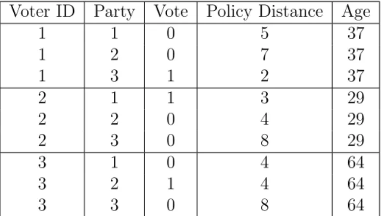
In order to be appropriate for a discrete choice model, data must have a unique obser-vation for each combination of case and alternative. This shape allows for choice-variant and choice-fixed variables. Suppose that a discrete choice model is used to examine the effect of policy distance and voters’ ages on their vote choices. In table 1.1, a row is defined by the unique combination of “Voter ID” and “Party.” The dependent variable “Vote” is 1 if the voter chooses to vote for the party being considered on that row, and is 0 otherwise. “Policy Distance” is choice-variant, but “Age” is choice-fixed.

Table 1.1: Example Discrete Choice Data.

Voter ID Party Vote Policy Distance Age

1 1 0 5 37

1 2 0 7 37

1 3 1 2 37

2 1 1 3 29

2 2 0 4 29

2 3 0 8 29

3 1 0 4 64

3 2 1 4 64

3 3 0 8 64

The simulations generate data that resemble voter-choice data as illustrated in table

(28)

1.1. I use two types of data generation processes. The first type, which I label “ba-sic,” uses a minimal number of covariates. Only 1 choice-variant covariate and only 1 choice-fixed covariate are used. As described in section 1.4.1, these covariates, as well as their coefficients, are drawn from uniform distributions. The second type, which I label “Britain,” follows the recommendation of Macdonald et al (2007) that, to the greatest extent possible, simulated data should resemble real data. Covariates are taken from the 1987 British Election Study, which has been used in a number of important political science papers on discrete choice methodology (Whitten and Palmer 1996; Alvarez and Nagler 1998; Quinn et al 1999; Alvarez et al 2000), and coefficients are drawn from the linear regression of party affect on these covariates. The Britain models are described in section 1.4.2. Both the basic and the Britain models simulate a dependent variable with 3 alternatives.

1.4.1 “Basic” Data Generation

The data generating processes are modeled on the random utility framework described in section 1.3. Each individual in the simulated data has a utilityUij for each alternative

which has a deterministic part Vij and a stochastic part εij. The deterministic part is

a linear combination of choice-variant and choice-fixed predictors. Vij also includes an

alternative-specific constant. In order to identify each model, one alternative is chosen to be the base alternative for which the coefficients for choice-fixed predictors and the alternative-specific constant are set to zero.

For the basic models, the evaluation of individual i of alternative j ∈ {1,2,3} is

Uij =λzij +βj,1xi+βj,0+εij, (1.9)

where candidate 1 is the base choice, requiring that β1,0 =β1,1 = 0. The choice-variant

(29)

from a uniform distribution from 0 to 1, but is held constant across the alternatives for each individual. Five “true” coefficients (λ, β2,0, β2,1, β3,0, and β3,1) are independently

drawn from a uniform distribution from −1 to 1.

The stochastic part of Uij consists of choice errors, ε1, ε2, and ε3, which are drawn

from a trivariate normal distribution:

ε1 ε2 ε3

0

∼N 0 0 0

0

,Σ

. (1.10)

The structure of the variance-covariance matrix of the choice errors, denoted by Σ, is crucial to the theoretical goals of the simulations. In these basic models, the variances in Σ are all set at one. I use 11 different correlation structures to represent a range of violations of the IIA assumption. Each structure implies a different matrix for Σ in equation 1.10. I present these error structures in section 1.4.3. The errors are drawn independently for individuals, but are correlated across the alternatives.

After all of the covariates, coefficients, and errors have been drawn, the simulated choice of an individual is the alternative with the highest latent utility for that individual. During each iteration of the simulation, a simulated data set is generated, then MNL, MXL, and MNP are run using the simulated choice as the dependent variable, z as a choice-variant predictor, and x as a choice-fixed predictor.7 The models are specified to include alternative-specific constants. The coefficients and standard errors from each model are saved, as well as the time for each model to converge, indicators for model non-convergence, predicted probabilities, and estimates of the parameters that account for error correlation. This information is used to assess the relative performance of each

7_{Multinomial logit is implemented by the “asclogit” command in Stata 11, and multinomial probit is}

(30)

estimator. The exact criteria on which the estimators are compared are described and results are reported in section 1.5. Each simulation is iterated 300 times for each of the 11 error correlation structures listed in section 1.4.3.

1.4.2 “Britain” Data Generation

For the Britain models I use the data from the 1987 British election study (Heath et al 1987). Indices for the alternatives are{C, L, A}, whereCrefers to the Conservative party,

Lrefers to the Labour party, andA refers to the Liberal/Social Democrat party alliance. For individual i, the deterministic part of the evaluation of alternative j ∈ {C,L,A} is a linear combination of 7 choice-variant predictors, 10 choice-fixed predictors, and alternative-specific constants:

Uij =

7

X

k=1

λkzijk+

10

X

l=1

βjlxil+βj,0+εij. (1.11)

To obtain realistic coefficients for λ and β in equation 1.11, I draw coefficients from a regression of the affect a respondent reports for each party, and the results from this regression are listed in table A.1 in Appendix A. The Conservative party is treated as the base alternative, so βC,0 = . . . = βC,10 = 0. The choice-variant z variables are

ideological distances between the respondents and the parties on defense, unemployment, taxation, nationalization, income redistribution, crime, and welfare. The choice-fixed x

variables are characteristics of the voters which include the respondent’s age, gender, income, geographic location, union membership, and homeowner status. More specific information about the variables included in the analysis are listed in Appendix A. The simulated choice of individualiis again the alternative with the highest associated utility. The stochastic part of Uij contains choice errors εC, εL, and εA. Again, the choice

(31)

correlation structures listed in section 1.4.3. The variances of the errors are also derived from the regression in table A.1 in Appendix A. The residuals from this regression are calculated and separated by the choice being considered. The variance-covariance matrix for the three vectors of residuals is

Σ =



    

1.133 . .

−0.406 1.127 .

−0.083 −0.039 0.604



    

. (1.12)

This matrix yields the correlation matrix

χ=



    

1 . .

−0.359 1 .

−0.100 −0.047 1



    

. (1.13)

The variances in 1.12 are used for the error variances in all of the Britain models, and the correlations in 1.13 are used as modelK in the error correlation structures described in section 1.4.3, which are applied to both the Britain and basic models.

The Britain simulations are also iterated 300 times for each error correlation structure listed in section 1.4.3. During each iteration, MNL, MXL, and MNP are run using the simulated choice as the dependent variable, the z variables as choice-variant predictors, and the x variables as choice-fixed predictors. As before, the models are specified to include alternative-specific constants. The same information is saved as in the basic simulations, and is also assessed as described and reported in section 1.5.

1.4.3 Error Correlation Structures

(32)

have variances equal to 1. For the Britain models, errors have the variances listed in equation 1.12. I consider 11 correlation models, which I call models A through K.

χA=      

1 . .

0 1 .

0 0 1

     

χB =      

1 . .

.10 1 . .10 .10 1

     

χC =      

1 . .

.25 1 . .25 .25 1

     

χD =      

1 . .

.50 1 . .50 .50 1

     

χE =      

1 . .

.75 1 . .75 .75 1

     

χF =      

1 . .

0 1 .

.80 0 1

     

χG =      

1 . .

0 1 .

−.80 0 1

     

χH =      

1 . .

0 1 .

.50 .80 1

     

χI =      

1 . .

0 1 .

−.50 .80 1

     

χJ =      

1 . .

−.20 1 .

−.50 .80 1

     

χK =      

1 . .

−0.359 1 .

−0.100 −0.047 1

     

Models A, F, G, H, I, and J were considered by Alvarez and Nagler (1994). Models E

(33)

1.5 Results and Discussion

The primary focus of this analysis is to determine which estimator produces the best coefficients. I analyze the performances of MNL, MXL, and MNP in returning accurate coefficient point estimates with the correct signs. These results are listed in section 1.5.1. In section 1.5.2, I compare the three estimators on several other criteria which are of interest to researchers in the field: inferences, the rate at which each estimator fails to converge to meaningful results, the time it takes for each estimator to converge, and the accuracy of predicted probabilities and parameters which account for error correlations. It can be argued that the results presented here are idiosyncratic to Stata, or to the particular estimation technique through which MNP is operationalized in Stata. To address these concerns, the simulations are rerun in R version 2.6.1 on exactly the same data.8 _{These results are reported in Appendix B. MNP is implemented in R within}

the “MNP” library, written by Imai and van Dyk (2005), and uses a Gibbs Sampler rather than simulated MLE to estimate choice probabilities. In general, Bayesian MNP in R is less stable than MNP in Stata, and becomes more likely to produce an error and terminate as the number of draws in the Gibbs Sampler increases. When the estimator does converge, the results are very similar to the ones presented in section 1.5.1.

1.5.1 Comparison of Coefficient Estimates

MNL, MNP, and MXL are estimators of the probability that, for each individual i and each alternativej, individualiselects alternative j. However, these probabilities are not the first concern for most researchers who employ discrete choice models. As with most multivariate empirical models, researchers are mainly concerned with the magnitude and direction of coefficient estimates returned by the model. The fit of model probabilities

8_{Only MNL and MNP are compared in R. I was unable to find a reliable implementation of MXL in}

(34)

is a secondary concern which illuminates the robustness of coefficient estimates. For example, an analyst of an election will be primarily concerned with how covariates are estimated to be associated with vote choice. The analyst may test whether voters with greater income are more likely to vote for a right-wing party, and if this effect is larger than the effect of regular church attendance. In choosing between MNL, MNP, and MXL, most researchers will want to choose the method that most reliably returns coefficients.

Comparing the accuracy of coefficient estimates in discrete choice estimators is dif-ficult because each estimator makes assumptions about the error variances which scale coefficients by an unknown factor. A straight comparison of point estimates to the true parameter values used in the generation of the data is impossible, since the actual error cannot be separated from the deviation due to scaling. In order to assess the error in coefficient point estimates in this analysis, a statistic which is similar to a Pearson corre-lation is calculated between the vector of true coefficient values and the vector of point estimates from each of MNL, MXL, and MNP.

Formally, the derivation of this comparative statistic is as follows. Each estimator returns a vector of K non-constrained coefficient estimates. In the basic simulation models, K = 5 since we estimate one effect for a choice-variantX variable, one constant for each non-base alternative, and one effect for a choice-fixed X variable for each non-base alternative. In the Britain models, K = 29 since there are 7 choice-variant X

variables, and a constant and 10 choice-fixed X variables for both non-base alternatives. For each model, the vector of true parameter values {β1, β2, . . . , βK} is saved, and the

vectors of point-estimates from each estimator {δˆ1,δˆ2, . . . ,

¯ ˆ

δK} are saved. It is assumed

that the returned coefficient estimates are scaled by the fixed standard deviation of each estimator, denoted σ. Therefore we can represent the returned estimate as a quotient of an estimate which is comparable to the true effect and the standard deviation:

ˆ

δ= ˆ

β

(35)

In order to eliminate σ from these estimates, we calculate the mean across the estimates for each model,δ¯ˆ, and compute

PK

i=1(ˆδi−δ¯ˆ)(βi−β¯) q

PK

j=1(ˆδi−

¯ ˆ

δ)2qPK

j=1(βi−β¯)2

= PK i=1 ˆ βi σ − ¯ ˆ β σ

(βi−β¯) s PK j=1 ˆ βi σ − ¯ ˆ β σ 2_q PK

j=1(βi−β¯)2

=

1

σ

PK

i=1( ˆβi−

¯ ˆ

β)(βi−β¯)

1

σ q

PK

j=1( ˆβi−

¯ ˆ

β)2qPK

j=1(βi−β¯)2

=

PK

i=1( ˆβi−

¯ ˆ

β)(βi−β¯) q

PK

j=1( ˆβi−

¯ ˆ

β)2qPK

j=1(βi−β¯)2

.(1.15)

The standard deviation cancels from the top and bottom of this fraction. This correlation statistic, reported in table 1.2, removes the constant scaling parameter and provides the desired information: if estimates differ from true parameter values only because of the scale, the correlation is 1. Lower correlations represent correspondingly less accurate co-efficient estimates.9 Unlike the point estimates, the signs and inferences of the coefficient estimates are naturally meaningful since they do not depend on an assumed variance. The average percent of coefficients for which each estimator returns the correct sign is reported in table 1.3.

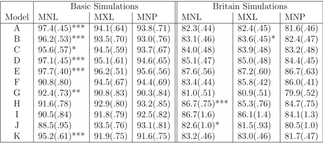
In tables 1.2 and 1.3, the evaluative statistic is reported for MNL, MXL, and MNP, for the basic and the Britain models, and for each of the 11 error correlation structures. The standard error of the mean for each measurement is reported, and two-tailed t tests are conducted. Stars indicate that one estimator performs significantly better than both competitors.

MNL returns more accurate coefficients than MXL and MNP in the majority of cases. In the basic models, which contain a minimum number of covariates, point estimates from

9_{Two other measures were used to compare coefficient estimates while removing the scale. The first}

(36)

Table 1.2: Correlations Between Coefficient Estimates from MNL, MXL, and MNP and the True Coefficients.

Basic Simulations Britain Simulations

Model MNL MXL MNP MNL MXL MNP

A 0.98(.00)*** 0.93(.01) 0.92(.01) 0.51(.01)*** 0.45(.01) 0.40(.01) B 0.98(.00)*** 0.94(.01) 0.91(.01) 0.54(.01)*** 0.49(.01) 0.44(.01) C 0.98(.00)*** 0.95(.01) 0.93(.01) 0.53(.01)*** 0.48(.01) 0.43(.01) D 0.98(.00)*** 0.95(.01) 0.93(.01) 0.55(.01)*** 0.50(.01) 0.46(.01) E 0.98(.00)*** 0.97(.00) 0.96(.01) 0.56(.02)*** 0.51(.02) 0.49(.02) F 0.88(.01) 0.94(.01)* 0.93(.01) 0.41(.01) 0.48(.01) 0.48(.01)** G 0.94(.01)** 0.92(.01) 0.90(.01) 0.54(.01)*** 0.44(.01) 0.41(.01) H 0.88(.01) 0.93(.01) 0.94(.01) 0.59(.02)*** 0.52(.02) 0.48(.02) I 0.86(.01) 0.93(.01) 0.93(.01) 0.58(.03)*** 0.48(.03) 0.44(.04) J 0.84(.01) 0.93(.01) 0.92(.01) 0.58(.02)*** 0.48(.02) 0.44(.02) K 0.97(.00)*** 0.93(.01) 0.91(.01) 0.53(.01)*** 0.47(.01) 0.41(.01)

Note: stars indicate that the marked correlation is significantly greater than the next highest correlation.

Two-tailedt tests: ***p < .01, **p < .05, *p < .1

Table 1.3: Percent Correct Signs of Coefficient Estimates from MNL, MXL, and MNP.

Basic Simulations Britain Simulations

Model MNL MXL MNP MNL MXL MNP

A 97.4(.45)*** 94.1(.64) 93.8(.71) 82.3(.44) 82.4(.45) 81.6(.46) B 96.2(.53)*** 93.5(.70) 93.0(.76) 83.1(.46) 83.6(.45)* 82.4(.47) C 95.6(.57)* 94.5(.59) 93.7(.67) 84.0(.48) 83.9(.48) 83.2(.48) D 97.1(.45)*** 95.1(.61) 94.6(.65) 85.1(.47) 85.0(.48) 84.4(.45) E 97.7(.40)*** 96.2(.51) 95.6(.56) 87.6(.56) 87.2(.60) 86.7(.63) F 90.8(.80) 94.5(.67) 94.4(.69) 83.4(.44) 85.8(.42) 86.0(.41) G 92.4(.73)** 90.8(.83) 90.3(.84) 81.0(.51) 80.9(.51) 79.9(.52) H 91.6(.78) 92.9(.80) 93.2(.85) 86.7(.75)*** 85.3(.76) 84.7(.75) I 90.5(.84) 91.8(.79) 92.5(.82) 86.7(1.6) 86.1(1.4) 84.1(1.3) J 88.5(.95) 93.5(.76) 93.1(.81) 82.6(1.0)* 81.5(.93) 80.5(1.0) K 95.2(.61)*** 91.9(.75) 91.6(.75) 83.2(.46) 83.0(.46) 81.7(.47)

Note: stars indicate that the marked value is significantly greater than the next highest value. Two-tailedt tests: ***p < .01, **p < .05, *p < .1

(37)

the most realistic correlation structure (model K). MXL and MNP have more accurate coefficients when a pair of errors are highly and positively correlated (models F, H, I, and J), and there is little difference between MXL and MNP in these cases.

However, in the Britain models MNL is more accurate in estimating the magnitude of coefficients for every correlation structure except F, which represents the unlikely situation that two alternatives are correlated at .8 while being independent from the third alternative. Likewise, with the exception of model F, MNL returns the correct signs more often than MNP, although there is little difference between MNL and MXL in these cases.

Violations of the IIA assumption have the expected effect on MNL estimates for the basic models: coefficient estimates are less accurate for the error correlation structures with large, positive correlations. Neither MXL or MNP are affected by IIA violations in such a systematic way. Comparing the basic model results to the Britain model results, however, it appears that the three estimators are hurt by the complexity of the Britain models, and MXL and MNP are hurt more by this complexity than MNL. Strangely, violation of IIA does not damage MNL estimates in the Britain models as it does in the basic models. In fact, MNL performs somewhat better with the highly correlated structures in the Britain models.

(38)

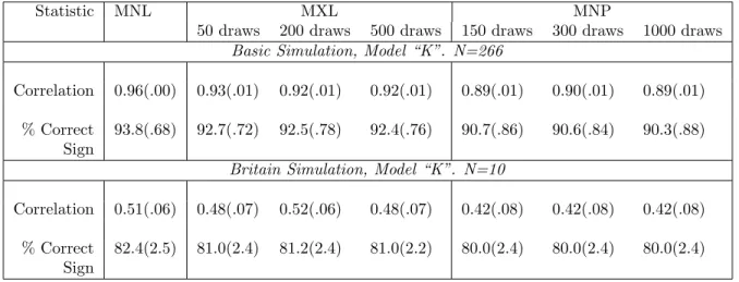
the estimators improves. I tested the increase in draws using correlation modelK, as the most realistic correlation model. Increasing the number of draws results in an increase in the time it takes each estimator to converge, so it was only feasible to run a large number of iterations for the basic models. I also ran 10 iterations for the Britain models. These results are reported in table 1.4.

Table 1.4: Evaluation Statistics for the Three Estimators, Increasing the Number of Draws.

Statistic MNL MXL MNP

50 draws 200 draws 500 draws 150 draws 300 draws 1000 draws

Basic Simulation, Model “K”. N=266

Correlation 0.96(.00) 0.93(.01) 0.92(.01) 0.92(.01) 0.89(.01) 0.90(.01) 0.89(.01) % Correct 93.8(.68) 92.7(.72) 92.5(.78) 92.4(.76) 90.7(.86) 90.6(.84) 90.3(.88)

Sign

Britain Simulation, Model “K”. N=10

Correlation 0.51(.06) 0.48(.07) 0.52(.06) 0.48(.07) 0.42(.08) 0.42(.08) 0.42(.08) % Correct 82.4(2.5) 81.0(2.4) 81.2(2.4) 81.0(2.2) 80.0(2.4) 80.0(2.4) 80.0(2.4)

Sign

The estimators do not consistently improve with more draws. In fact, as MXL moves from 200 to 500 draws and MNP moves from 300 to 1000 draws they both perform slightly less well, though not significantly so. These results suggest that the fact that MNL outperforms MXL and MNP is not due to the number of draws used to estimate MXL and MNP.

1.5.2 Additional Comparisons

(39)

frequency with which they fail to converge to meaningful results, and the time it takes each estimator to converge. Finally, since much of the work to compare MNL and MNP has focused on model fit and substitution patterns, the estimators are compared in the accuracy of their predicted probabilities and estimates of parameters to account for error correlation.

Inferences.

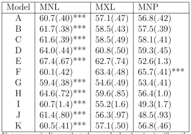
Inferences are difficult to gage using simulated data since the true parameters are specified with no variance or uncertainty. In order to generate a baseline against which to compare the inferences of MNL, MXL, and MNP coefficient estimates, I use the inferences from the regression on party affect from the 1987 British election study listed in table A.1 in Appendix A. Party affect is conceptually similar to the latent utilities which are used to generate the simulated dependent variables in the Britain models, described in section 1.4.2, and these models use the same predictors for the simulated vote choice as the ones that party affect is regressed on. As an illustrative exercise, it is reasonable to expect the estimators to return the same signs and inferences for the covariates as reported in the regression.

(40)

Table 1.5: Percent Correct Inferences on Coefficient Estimates from MNL, MXL, and MNP.

Model MNL MXL MNP

A 60.7(.40)*** 57.1(.47) 56.8(.42) B 61.7(.38)*** 58.5(.43) 57.5(.39) C 61.6(.39)*** 58.5(.49) 58.1(.41) D 64.0(.44)*** 60.8(.50) 59.3(.45) E 67.4(.67)*** 62.7(.74) 52.6(1.3) F 60.1(.42) 63.4(.48) 65.7(.41)*** G 59.4(.38)*** 54.6(.49) 53.4(.41) H 64.6(.72)*** 59.6(.85) 56.4(1.0) I 60.7(1.4)*** 55.2(1.6) 49.3(1.7) J 61.4(.80)*** 56.3(.97) 48.5(.93) K 60.5(.41)*** 57.1(.50) 56.8(.46)

Note: stars indicate that the marked value is significantly greater than the next highest value. Two-tailedt tests:

*** p < .01, **p < .05, *p < .1

Failure Rates and Time to Convergence.

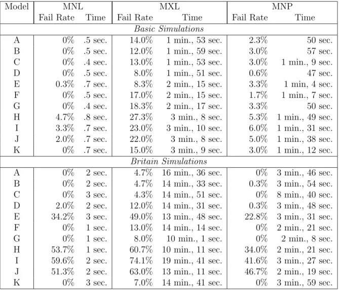
Concerns about the consistency of parameter or probability estimates are moot if an estimator fails to produce usable results, or if the model cannot converge in a practical amount of time. The failure rate and convergence time for each estimator are not defini-tive criteria on which to choose between MNL, MXP and MNP. However, they must be considered while comparing the estimators in other ways. The failure rates for the three estimators as well as the average convergence time of each estimator, omitting failed attempts, are reported in table 1.6 for each of the 22 simulations.

(41)

Table 1.6: Failure Rates and Average Time to Successfully Converge for MNL, MXL, and MNP.

Model MNL MXL MNP

Fail Rate Time Fail Rate Time Fail Rate Time

Basic Simulations

A 0% .5 sec. 14.0% 1 min., 53 sec. 2.3% 50 sec.

B 0% .5 sec. 12.0% 1 min., 59 sec. 3.0% 57 sec.

C 0% .4 sec. 13.0% 1 min., 53 sec. 3.0% 1 min., 9 sec.

D 0% .5 sec. 8.0% 1 min., 51 sec. 0.6% 47 sec.

E 0.3% .7 sec. 8.3% 2 min., 15 sec. 3.3% 1 min, 4 sec.

F 0% .5 sec. 17.0% 2 min., 15 sec. 1.7% 1 min., 7 sec.

G 0% .4 sec. 18.3% 2 min., 17 sec. 3.3% 50 sec.

H 4.7% .8 sec. 27.3% 3 min., 8 sec. 5.3% 1 min., 49 sec.

I 3.3% .7 sec. 23.0% 3 min., 10 sec. 6.0% 1 min., 31 sec.

J 2.0% .7 sec. 22.0% 3 min., 8 sec. 5.0% 1 min., 38 sec.

K 0% .7 sec. 15.0% 3 min., 9 sec. 3.0% 1 min., 12 sec.

Britain Simulations

A 0% 2 sec. 4.7% 16 min., 36 sec. 0% 3 min., 46 sec.

B 0% 2 sec. 4.7% 14 min., 33 sec. 0.3% 3 min., 54 sec.

C 0% 3 sec. 4.3% 14 min., 51 sec. 0% 8 min., 40 sec.

D 2.0% 2 sec. 12.0% 14 min., 31 sec. 0.3% 3 min., 48 sec.

E 34.2% 3 sec. 49.0% 13 min., 48 sec. 22.8% 3 min., 31 sec.

F 0% 1 sec. 13.0% 14 min., 14 sec. 0% 2 min., 21 sec.

G 0% 1 sec. 8.0% 10 min., 1 sec. 0% 2 min., 8 sec.

H 53.7% 1 sec. 60.7% 10 min., 11 sec. 34.0% 2 min., 21 sec.

I 59.6% 2 sec. 74.1% 19 min., 41 sec. 41.6% 3 min., 27 sec.

J 51.3% 2 sec. 63.0% 13 min., 11 sec. 46.7% 2 min., 19 sec.

K 0% 3 sec. 7.0% 14 min., 41 sec. 0% 3 min., 59 sec.

errors,10 _{and too many iterations without improvement in the log-likelihood function.}11

In addition, each estimator is marked to have failed if it produces an error and terminates without producing results.

10_{A run of an estimator is marked as failed if the trace of the variance matrix of coefficient estimates}

is greater than 100. This statistic captures any instance in which a standard error is infeasibly large for the simulated data.

11_{MNP is coded as failed if it takes more than 16,000 iterations to converge. MXL tends to converge}

(42)

MNL should converge more quickly than the other two estimators since choice proba-bilities do not need to be approximated numerically. The results in table 1.6 demonstrate that, as expected, MNL is much quicker, although none of the estimators ever take more than 20 minutes to converge on average. MXL consistently has a higher failure rate than MNP, which tends to fail more often than MNL. However, the three estimators share the cases in which their failure rates are highest, and these situations involve higher error correlations (models E,H,I, andJ). These models reflect weaker identification of error covariance elements, and cause MNL, which is normally very stable, to fail at high rates just like MNP and MXL. Since these models represent overly severe violations of IIA, the fail rates do not provide conclusive evidence to use one estimator over another in the three choice case.

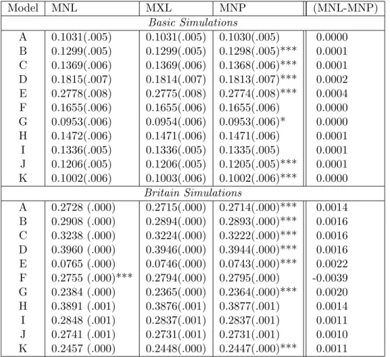
Predicted Probabilities.

The fit of a discrete choice model can be assessed by the magnitude of probability es-timates for the alternatives which are actually chosen in the data. A standard way to choose between models is to select the one with the best fit. However, there is a danger that a model may overfit the data, and provide probability estimates which are more certain than is appropriate. In the simulations used in this analysis, uncertainty is built into the simulated choice, therefore “correct” choice probabilities can be computed.12

The predicted probabilities from MNL, MXL, and MNP are calculated for each run, and are assessed for their mean squared error with the true choice probabilities. The average errors for each estimator and each correlation structure are reported in table 1.7.

MNP is consistently estimating the choice probabilities with less error than MNL or

12_{Given the known values of coefficient and error covariance parameters, the correct values for the}

predicted choice probabilities are given by the CDF of the multivariate normal distribution. The choice probability for choice 1 in these simulations is the bivariate normal CDF with arguments η2/ση2 and

η3/ση3 as defined in equations 1.3 and 1.7, and correlation ρ as defined in equation 1.8. The

(43)

Table 1.7: Errors in Predicted Probabilities from MNL, MXL, and MNP.

Model MNL MXL MNP (MNL-MNP)

Basic Simulations

A 0.1031(.005) 0.1031(.005) 0.1030(.005) 0.0000

B 0.1299(.005) 0.1299(.005) 0.1298(.005)*** 0.0001

C 0.1369(.006) 0.1369(.006) 0.1368(.006)*** 0.0001

D 0.1815(.007) 0.1814(.007) 0.1813(.007)*** 0.0002

E 0.2778(.008) 0.2775(.008) 0.2774(.008)*** 0.0004

F 0.1655(.006) 0.1655(.006) 0.1655(.006) 0.0000

G 0.0953(.006) 0.0954(.006) 0.0953(.006)* 0.0000

H 0.1472(.006) 0.1471(.006) 0.1471(.006) 0.0001

I 0.1336(.005) 0.1336(.005) 0.1335(.005) 0.0001

J 0.1206(.005) 0.1206(.005) 0.1205(.005)*** 0.0001

K 0.1002(.006) 0.1003(.006) 0.1002(.006)*** 0.0000

Britain Simulations

A 0.2728 (.000) 0.2715(.000) 0.2714(.000)*** 0.0014

B 0.2908 (.000) 0.2894(.000) 0.2893(.000)*** 0.0016

C 0.3238 (.000) 0.3224(.000) 0.3222(.000)*** 0.0016

D 0.3960 (.000) 0.3946(.000) 0.3944(.000)*** 0.0016

E 0.0765 (.000) 0.0746(.000) 0.0743(.000)*** 0.0022

F 0.2755 (.000)*** 0.2794(.000) 0.2795(.000) -0.0039

G 0.2384 (.000) 0.2365(.000) 0.2364(.000)*** 0.0020

H 0.3891 (.001) 0.3876(.001) 0.3877(.001) 0.0014

I 0.2848 (.001) 0.2837(.001) 0.2837(.001) 0.0011

J 0.2741 (.001) 0.2731(.001) 0.2731(.001) 0.0010

K 0.2457 (.000) 0.2448(.000) 0.2447(.000)*** 0.0011

Note: stars indicate that the value is significantly lower than the next lowest value. Two-tailedt tests: ***p < .01, **p < .05, *p < .1

(44)

generally result in a better fit.13

Parameters Which Account for Error Correlation.

One important reason why researchers may prefer MXL or MNP to MNL is that the more general MXL and MNP models allow estimation of substitution effects. That is, individuals may consider some alternatives to be more suitable replacements than others for an alternative that drops out of the analysis for reasons which are not specified in the model. These substitution patterns can be analyzed by deriving the marginal effect of covariates on the predicted probabilities when the utility for the “irrelevant” alternative is normalized to 0. However, these patterns are only reliable if the model can accurately estimate the correlation structure of the error. As noted in equation 1.8, neither MXL nor MNP can return individual elements of the error correlation matrix, but they can account for the correlation by estimating the correlation of residual differences. The true correlation values in table 1.8 are derived by evaluating equation 1.8 using the error covariance elements assumed by each model. Stars in this table indicate that the estimator produces a correlation point estimate which is on average significantly different from the correct value.

MNP appears, in general, to estimate the correlation parameter more accurately than MXL. In the Britain models, which are more complicated, MXL becomes much less reliable but MNP does not seem to suffer any worse than in the basic models. Note however that correlation estimates from MNP are biased downwards in every model. It may be the case that MNP correlation estimates are biased downwards in general.

13_{A good way to test whether MNP really does produce more accurate estimates of predicted}

(45)

Table 1.8: Comparison of Parameter Estimates Which Account for Error Correlation.

Basic Simulations Britain Simulations Model True Value MXL MNP True Value MXL MNP

A 0.50 0.30(.05)*** 0.45(.03) 0.57 -0.02(.05)*** 0.54(.02)* B 0.50 0.33(.04)*** 0.44(.03)** 0.57 -0.01(.04)*** 0.53(.02)** C 0.50 0.36(.04)*** 0.42(.03)*** 0.57 0.11(.05)*** 0.55(.02) D 0.50 0.33(.04)*** 0.44(.02)** 0.56 0.06(.04)*** 0.53(.02) E 0.50 0.32(.04)*** 0.45(.02)** 0.54 0.14(.09)*** 0.45(.04)* F 0.22 -0.00(.04)*** 0.18(.03) 0.51 0.25(.05)*** 0.49(.03) G 0.67 0.52(.05)*** 0.60(.03)*** 0.68 0.39(.06)*** 0.58(.03)*** H 0.92 0.90(.02) 0.86(.02)*** 0.96 0.65(.07)*** 0.80(.03)*** I 0.94 0.75(.04)*** 0.83(.02)*** 0.92 0.54(.12)*** 0.75(.06)*** J 0.93 0.83(.03)*** 0.85(.02)*** 0.92 0.68(.12)* 0.85(.03)** K 0.58 0.43(.05)*** 0.52(.03)* 0.65 0.14(.04)*** 0.62(.02)

Note: stars indicate that the correlation is significantly different from the correct value. Two-tailedt tests: ***p < .01, **p < .05, *p < .1

1.6 Conclusion

The choice between MNL, MXL, and MNP should depend on the goal of the researcher. If the goal is to interpret the effects of covariates on the discrete choice, then the simulations presented here indicate that, in most situations, MNL provides more accurate point estimates than MXL or MNP even when the IIA assumption is severely violated. If the goal is to estimate choice probabilities, then the simulations suggest that MNP provides an improvement over MNL and MXL, but at the expense of the coefficient estimates. The error-components version of MXL used here rarely outperforms MNL and MNP in these simulations, but if the goal is to model the effects of covariates as random with a known distribution, then a random-slope version of MXL may well be the best option.

(46)

the errors modeled by MNP and MXL is correlation between random variables which represent noise. Therefore, by definition, we do not have any theory to explain error correlation, or else we should have included that information in the deterministic part of the model. A thoughtful model which includes variables that capture perceived similarity between choices will be less likely to violate IIA.

(47)

Chapter 2 Drawing Accurate Inferences About

the Differences Between Cases in

Time-Series Cross-Section Data

2.1 Summary

(48)

Simulations demonstrate that BEER is more accurate than the other commonly used TSCS methods when the goal of the researcher is to model cross-sectional effects that change in a smooth way over time.

2.2 Introduction

Time-series cross-section (TSCS) data contain a cross-section of N cases, measured at each ofT time points, and have two variances: a variance across the cases, and a variance across time. Studies that use TSCS data are becoming increasingly prevalent in political science. In American politics, many studies consider the 50 states over a time span. In comparative politics and international relations, these data take the form of countries and years. While a cross-sectional dataset may have a sample size of N, and a time-series can contain T observations of one case, TSCS data can have as many as N ×T

observations. This increase in power is part of the reason why TSCS methods have become so popular, but different TSCS methods make different generalizations within the data; TSCS methods allow us to generalize across cases, across time, or both if it is appropriate to do so. Political researchers need to be aware of the assumptions being made by their methods, and they need to be more careful to choose a method which makes theoretically appropriate assumptions.1

In choosing an appropriate method, researchers should first be aware that different

1_{Choosing a method can be difficult. A great deal of confusion arises with TSCS methodology because}

(49)

TSCS methods are designed to produce inferences about different aspects of the data. Many commonly used methods consider only the variation over time. Some consider only the variation across cases, and others draw inferences by averaging the two dimensions of variance. A method which analyzes the cross-sections should not in general be expected to produce the same results as a method which analyzes time variation. Since inferences on the cross-sectional and time variation are different, an average of the two will not typically provide accurate results on either dimension.

LetX refer generally to an independent variable in a linear model, and letY refer to the dependent variable. In this discussion I will use the following terminology:

• Between Effect: the effect of X on cross-sectional differences inY;

• Within Effect: the effect of X on changes inY over time.

There is no reason why these two effects should necessarily be equal, and there are many situations in fact when the two effects might be expected to be in opposite directions. Figure 2.1 contains an illustration of hypothetical TSCS data in which the between and

Figure 2.1: Within Effects, the Between Effect of Case-Level Averages, and the Overall OLS Effect.

Within Effects Average Between Effect Overall OLS Effect

Note: The graphs are scatterplots of hypothetical data which include five cases, measured at 25 time points each. The 25 observations of each case are denoted by the

(50)

within effects have different signs. Each graph is a scatterplot with an overlaid best-fit regression line. In the graph on the left, the within effects are drawn. These slopes capture the fact that within each case, increases inX are associated with decreases inY. A between effect is drawn on the graph in the middle which is derived from the average values of X and Y within each case. This line illustrates the fact that at any point in time, a case with a higher value ofX than another case also tends to have a higher value ofY. The graph on the right contains the standard OLS best-fit line, which is an average of the between and within slopes, and fails to accurately depict the variation along either dimension.

In this paper, I develop a new method for researchers who are interested in estimating the between effects in TSCS data. Commonly used TSCS methods are discussed in section 2.3, including a few which estimate between effects. The new method discussed here, however, allows a researcher to model something that the other methods do not: the between effects are allowed to vary over time.

Political theory should suggest a model for how data are generated. This goal of this research is to develop a TSCS method to estimate a model in which the between effects are estimated and are allowed to change over time in a smooth fashion. Formally, this data-generating model can be represented as follows:

yit=αt+xitβt+εit, εit ∼N(0, σt2), (2.1)

Cov(βt, βt−1)>0, ∀t > t1,

wherei∈ {1, . . . , N}denotes cases, t∈ {t1, . . . , T}denotes time points,yit is the

depen-dent variable, xit is a column vector of independent variables, αt and σt2 are scalar, and

βt is a column vector of between effects. The parameters αt, βt, and σt2 are all allowed

(51)

adjacent time points. The within variation is entirely accounted for by the time-specific constantsαt so that the regression coefficients only provide estimates of between effects.

The method developed here to estimate this model is called the between effects estima-tion routine (BEER), and it is designed to estimate the between effects in a particular time point while maximizing the amount of information in the TSCS data used to make these estimates. The algorithm focuses solely on the between effects of predictors by “de-pooling” the data, running OLS on individual cross-sections, and using conjugate Bayesian priors to average results across the cross-sections. The formulation of BEER is discussed in detail in section 2.4.

(52)

In the second example, described in section 2.6, BEER is used to analyze the effect of median state income on the state’s votes in U.S. presidential elections from 1964 to 2004. Andrew Gelman et al (2008) find that Democrats receive higher percentages of the vote in richer states relative to poorer states. They also show, however, that this between effect has only emerged in the last 20 years. The growing importance of income as a predictor of state-level voting concords with other theories about political polarization in the American electorate. Income, perhaps, is an indicator of diverging cultures between the states, which would imply that these differences are much more pronounced now than in 1964.

In both of these examples, the research question calls for the analysis of between effects, and theory requires that these effects be allowed to vary over time in a smooth fashion. BEER assumes this exact model, and therefore should return more accurate results than other TSCS methods which do not assume this model. In order to test the robustness of BEER against alternative TSCS methods in a more general setting, simulations are run. These simulations, presented in section 2.7, generate artificial data using four different models, including the one described in equation 2.1. The simulations demonstrate that BEER is the most accurate alternative when the model in equation 2.1 is the true data generating process.

2.3 Background

(53)

All models for TSCS data use the following equation:

yit=g(αit, βit, xit) +ui+vt+eit, (2.2)

where g(.) is a function of the predictors xit, an intercept αit, and coefficients βit. When

the intercept and coefficients are fixed across time and across cases, and when g(.) is a linear function of xit, this model is called the pooled model (Cameron and Trivedi 2005,

p. 699). There are PN

i=1Ti total observations. The overall residual for the model is

εit =ui+vt+eit, whereui is the unobserved variance of yit that varies across cases but

is fixed across time, andvt is the unobserved variance ofyit that varies across time but is

fixed across cases. These values are also called unit effects, or unobserved heterogeneity.

eit is the idiosyncratic error, which varies over time and across panels. In the discussion

in this section, I assume that the residuals are independent of the regressors. This assumption would imply that Corr(xit, ui) = 0, which may be controversial, but only if

endogeneity is a concern for an OLS regression within an individual cross-section in the data.

There are many options for researchers who have TSCS data and want to choose an estimator for the model in equation 2.2. Before discussing what distinguishes the different methods for TSCS data, however, it will be useful to define between and within variables. Any variable xit that varies across cases and over time can be separated into

parts which capture only the cross-sectional variation and only the temporal variation of xit. The cross-sectional part of xit is called a between variable, and its effect in a

regression model is strictly a between effect as defined in section 2.2. One way to create a between variable is to take the average value of the variable over time for each case:

xB_i =

PTi t=1xit

Ti

(54)

These variables are fixed over time, but have a variance between the cases. Note that the between effects are defined to be averages over the measured time frame. The temporal part of xit is called a within variable, and its effect in a regression is strictly a within

effect. One way to construct a within variable is to subtract the between variable from the whole variable:

xW_it =xit−xBi . (2.4)

The within variable centers xit around its mean for each case, so that average differences

between cases are removed. The differences over time, however, are preserved. Notice that, by these definitions, any variable which varies over time and cross-sectionally is the sum of its between and within parts:

xit =xBi +x W

it. (2.5)

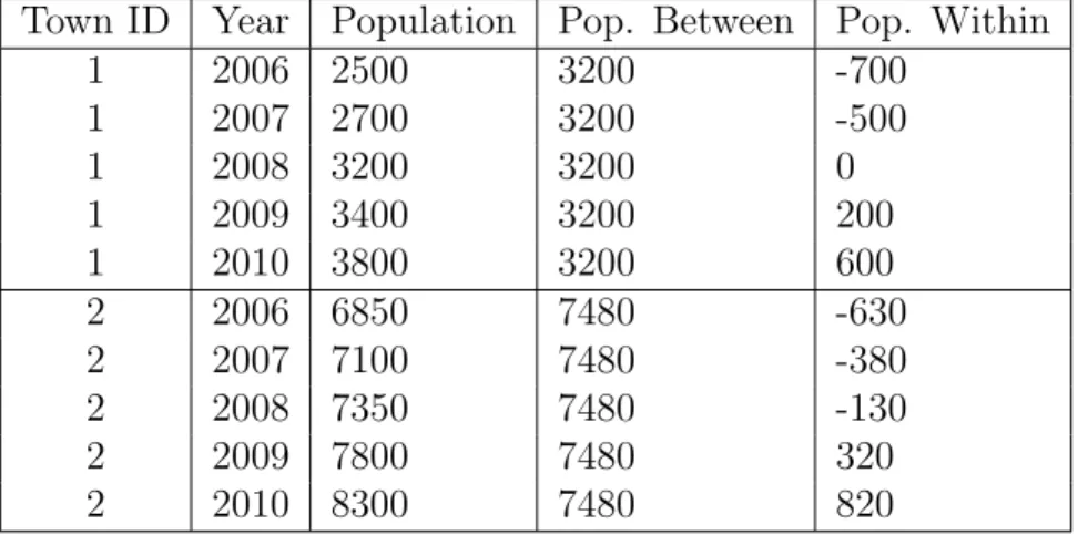
Table 2.1 provides an example of how to calculate these between and within parts of a TSCS variable. Suppose we have data on the population of two towns from 2006 to 2010. Both towns are growing, but town 2 is always bigger than town 1. The between version of population is the average population of each town over the five year period. This variable captures the fact that town 2 is bigger than town 1. The within version of population is the difference between the populations and each town’s average population. This variable preserves year to year differences within each town – the population of town 1 grew by 200 people between 2006 and 2007, and so did the within version of population – but eliminates meaningful differences between town 1 and town 2.

(55)

Table 2.1: Example of Between and Within Parts of a Variable in TSCS Data Town ID Year Population Pop. Between Pop. Within

1 2006 2500 3200 -700

1 2007 2700 3200 -500

1 2008 3200 3200 0

1 2009 3400 3200 200

1 2010 3800 3200 600

2 2006 6850 7480 -630

2 2007 7100 7480 -380

2 2008 7350 7480 -130

2 2009 7800 7480 320

2 2010 8300 7480 820

second category refers to methods which estimate between and within effects separately in the same model, and includes fixed effects with vector decomposition (Plumper and Troeger 2007), and the approach described by Yair Mundlak (1978). The third category estimates the within effects only, and ignores the between effects entirely. Much of the recent work in the development of TSCS methods in political science falls within this category. Fixed effects estimators are classified in this group, as well as several variants such as error correction models (Keele and DeBouf 2008). Finally, the last category in-cludes models which estimate the between effects only, ignoring the within effects: the time effects estimator and the between estimator are the two most prominent examples in this group.