Deconvolution Estimation of a Mixture Distribution with
Boundary Effects Motivated by Mutation Effect Distribution
by Mihee Lee
A dissertation submitted to the faculty of the University of North Carolina at Chapel Hill in partial fulfillment of the requirements for the degree of Doctor of Philosophy in the Department of Statistics and Operations Research.
Chapel Hill 2009
Approved by:
J. S. Marron, Advisor
Haipeng Shen, Advisor
Edward Carlstein, Committee Member
Christina L. Burch, Committee Member
Jon W. Tolle, Committee Member
c ° 2009 Mihee Lee
ABSTRACT
MIHEE LEE: Deconvolution Estimation of a Mixture Distribution with Boundary Effects Motivated by Mutation Effect Distribution.
(Under the direction of J. S. Marron and Haipeng Shen.)
Density estimation in measurement error models has been widely studied. However, most
existing methods consider only continuous target variables, hence they cannot be applied
directly to many real problems. Motivated by an evolutionary biology study, we consider
more general cases: the target distribution is a mixture of a continuous component and finite
numbers of pointmasses, which can cover most of practical problems. In this dissertation, we
approach the estimation of the distribution in three different ways under the framework of
measurement error models.
Our first proposal is of the Fourier type, which is obtained by generalizing Liu and Taylor
(1989). The proposed estimator has a closed form, and gives continuous and smooth density
estimators for the continuous mixture component. In addition, its convergence rate is
compa-rably fast. However, when the target distribution has non-smooth boundaries, it suffers from
a strong boundary effect. This motivates us to to propose two other methods of the sieve type;
one is based on maximum likelihood (ML), and the other uses least squares (LS). By easily
reflecting the known boundary information, they remarkably reduce the boundary problems,
which is another major contribution of this dissertation. Moreover, the use of penalization
improves the smoothness of the resulting estimator, especially the ML based estimator, and
reduces the estimation variance.
For each estimator, some asymptotic properties are explored by mathematical
compu-tation, and finite sample performances are illustrated via simulation studies. In addition,
the proposed estimators are applied to the virus lineage data in Burch et al. (2007), which
originally motivates this study. In this application, we not only estimate the mutation effect
effect distribution, using density envelope plots.
ACKNOWLEDGEMENTS
This is a great opportunity to express my respect and gratitude to my advisors, Professor J. S.
Marron and Professor Haipeng Shen. I have been exceedingly fortunate to have advisors who
gave me the freedom to explore my own ideas, and offer invaluable guidance when my steps
faltered. They introduced me to new ways to express and cultivate my ideas, and to deeply
examine and question thoughts. Their patience and support helped me overcome many trials
leading to the completion of this dissertation. I hope one day to become as good of an advisor
to my students as they have been to me.
I would like to thank my other committee members, Christina Burch, Edward Carlstein,
Jon Tolle and Young Truong for their valuable suggestions on this dissertation. Especially, I
thank Christina for kindly providing the data set that led to an interesting application, and
Jon for helping me with the implementation of the proposed method. Furthermore, I would
like to express my gratitude to Peter Hall, who has been involved from the very beginning of
this work.
I also wish to acknowledge all the friends I met while in Chapel Hill. These friendships
helped me to weather the long hours spent in my office. Also, I want to extend appreciation
to my friends in Korea, who make me feel that they are always close even though we were
physically far apart. Finally, the acknowledgements would not be complete without a heart
felt thanks to my family, especially my parents, for their love and belief in me. I cannot thank
Contents
ACKNOWLEDGEMENTS v
List of Figures ix
List of Tables x
1 Introduction 1
2 Direct Deconvolution Estimation 5
2.1 Introduction . . . 5
2.2 The Proposed Estimators . . . 6
2.2.1 Estimation of the Pointmass p . . . 7
2.2.2 Density Estimation of the Continuous Component fc . . . 8
2.3 Asymptotic properties of the Proposed Estimators . . . 9
2.4 Simulation Studies . . . 14
2.4.1 Case 1: Mixture of N(3,1) and the Pointmass . . . 15
2.4.2 Case 2: Mixture of N(0,1) and the Pointmass . . . 18
2.4.3 Case 3: Mixture of Exp(1) and the Pointmass . . . 21
2.5 Application to the Virus-lineage Data . . . 23
2.5.1 Description on the data . . . 23
2.5.2 Analysis Results . . . 24
3 Sieve Type Deconvolution Based on Maximum Likelihood 36
3.1 Introduction . . . 36
3.2 Model and Methodology . . . 37
3.2.1 Model . . . 38
3.2.2 Basic Description of the Estimation Method . . . 39
3.2.3 A Standard Sieve Estimator . . . 40
3.2.4 A Penalized Sieve Estimator . . . 42
3.3 Consistency of the Proposed Estimators . . . 43
3.4 A Simulation Study . . . 46
3.4.1 Simulation Description . . . 46
3.4.2 Pointmass Estimation . . . 47
3.4.3 Continuous Distribution Estimation . . . 48
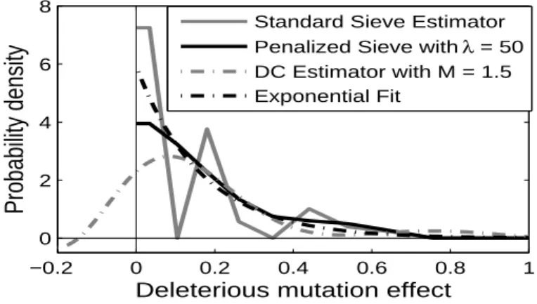
3.5 Application to the Virus-lineage Data . . . 50
3.5.1 Estimation Results . . . 50
3.5.2 Validation of the Exponential Assumption . . . 51
3.6 Proofs and Technical Details . . . 53
3.6.1 Proof of the Theorems . . . 54
3.6.2 Optimization details in the Sieve ML Estimation . . . 60
4 Sieve Type Deconvolution Based on Least Squares 63 4.1 Introduction . . . 63
4.2 The Proposed Estimators . . . 64
4.2.1 LS on Cumulative Distribution Functions . . . 66
4.2.2 LS on Characteristic Functions . . . 67
4.3 Theoretical Properties . . . 68
4.4 Simulation Studies . . . 69
4.4.1 Case 1: Correctly Specified Error Distribution . . . 70
4.4.2 Case 2: Misspecified Error Distribution . . . 73
4.6 Proofs and Technical Details . . . 77
4.6.1 Proof of Theorems . . . 77
4.6.2 Details on Implementing the Proposed Methods . . . 80
Future Work 82
Bibliography 86
List of Figures
2.1 Simulation 1: Direct deconvolution pointmass estimation . . . 15
2.2 Simulation 1: Direct deconvolution density estimation with the true p . . . . 17
2.3 Simulation 1: Direct deconvolution density estimation with ˆp . . . 18
2.4 Simulation 2: Direct deconvolution pointmass estimation . . . 19
2.5 Simulation 2: Direct deconvolution density estimation with the true p . . . . 20
2.6 Simulation 2: Direct deconvolution IMSE plot . . . 21
2.7 Simulation 3: Direct deconvolution pointmass estimation . . . 22
2.8 Simulation 3: Direct deconvolution density estimation with the true p . . . . 22
2.9 Direct deconvolution pointmass estimation in the virus data analysis . . . 25
2.10 Direct deconvolution density estimation in the virus data analysis . . . 26
3.1 Simulation: Sieve ML pointmass estimation . . . 48
3.2 Simulation: Sieve ML density estimation . . . 49
3.3 Virus lineage data - Comparison of three estimation methods . . . 51
3.4 Density-envelope plots - validation of the exponential assumption . . . 52
3.5 Bias and variance tradeoff for the PS-ML estimator . . . 54
4.1 Simulation 1: Performance of the LS-cdf with uniform weight function . . . . 70
4.2 Simulation 1: LS-cdf with non-uniform weight function . . . 72
4.3 Simulation 1: Performances of the LS-chf method . . . 72
4.4 Simulation 1: Effects of the parameter M in LS-chf . . . 73
List of Tables
Chapter 1
Introduction
Estimating the probability distribution of a random variable is one of the classical problems
in statistics. When some realizations of the random variable are given, many methods to
estimate its distribution have been developed from the classical statistical viewpoint. First, if
the distribution of the random variable comes from a known parametric family, or there are
good reasons to assume some specific distribution family as the truth, an assumed probability
distribution can be fit to the data by estimating only the unknown parameters. This process
is called parametric estimation. See, for example, Casella and Berger (2001) and Lehmann
and Casella (1998). When a parametric model is inappropriate, several methods have been
developed to estimate the distribution (Hastie et al., 2001). There is a large body of work
in this direction called nonparametric density estimation. Common methods in that area
include histogram, kernel smoothing, splines, etc.
When the information about the underlying distribution is correct, parametric estimation
is better than the nonparametric methods in two aspects. First of all, it is easier and needs
less amount of computation than the latter. Moreover, the convergence rate of the estimator is
faster in the case of parametric estimation. The drawback of parametric estimation is it highly
depends on the true distribution. That is, when the assumed true distribution is not correct,
its performance can be poor. On the other hand, nonparametric density estimation does not
need any assumption for the true distribution of the data except continuity or smoothness.
So, when there is little information about the underlying distribution, the nonparametric
The estimation of the distribution is particularly challenging when the true realizations
of the target variable are not observed. In this case, the classical distribution estimations
described above cannot be directly applied. LetXbe the random variable whose distribution
we want to estimate. Because of some reasons, we can observe only the error contaminated
variableY where
Y =X+Z, (1.1)
where Z is a measurement error with known probability density function fZ, and is
inde-pendent of the target variable X. To fit the underlying distribution based on the error
contaminated data, one naive method is to ignore the existence of the measurement error.
When the measurement error is much smaller than the target variable, the performance of
this approach is not too bad. However, when the measurement error is comparatively large,
so not negligible, this method can give an arbitrarily poor conclusion.
A better way is to take into account the existence of the measurement error and reduce
its effect from the observed data by using the known distribution information ofZ, which is
calleddeconvolution method. Such a problem has been widely studied whenX is a continuous
random variable having a continuous probability density function. There are large volume of
studies for the deconvolution problem.
Existing deconvolution methods fall into two groups: The first group is Fourier-based,
which uses ideas of Fourier- and Inverse Fourier transformations and kernel smoothing. For
detailed description of various methods and their asymptotic properties, see Devroye (1989),
Liu and Taylor (1989), Stefanski and Carroll (1990), van Es and Kok (1998), Wand (1998),
Hesse (1999), Delaigle and Gijbels (2002), Meister (2007), Hall and Meister (2007), Zhang
and Karunamuni (2008), Carroll and Hall (1988), Stefanski (1990), Fan (1991a,b) and so on.
The second group is for non-Fourier based methods. Many of such methods use basis
functions such as B-splines or wavelets to expand the target density (or distribution function),
before estimating the coefficients of the basis using various approaches. For example, see
Mendelsohn and Rice (1982), Koo and Park (1996), Cordy and Thomas (1997), Pensky and
and Staudenmayer et al. (2008). In addition, other alternatives have been proposed such as
NPMLE (Groeneboom and Wellner, 1992; van Es and van Zuijlen, 1996; Jongbloed, 1998),
SIMEX (Stefanski and Bay, 1996; Wagner and Stadtm¨uller, 2008), and TAYLEX (Carroll
and Hall, 2004; Wagner and Stadtm¨uller, 2008).
In this dissertation, motivated by an evolutionary biology study, we are particularly
inter-ested inX which has a mixture distribution with both discrete and continuous components.
That is, X can be represented as
X=
½
aj, with probabilitypj, for 1≤j≤ν,
Xc, with probabilitypν+1,
(1.2)
where the values of a1, . . . , aν are known constants, and Xc is a continuous random variable with the density functionfc. Then, estimating the distribution ofXis equivalent to estimating
bothp= (p1, . . . , pν+1)T and the densityfc. Here, eachpj is the unknown mixing probability, hence the estimation of p can be understood as the estimation of the mixture proportion. However, our problem is quite different from the challenging classical mixture distribution
estimation problems (McLachlan and Basford, 1988; McLachlan and Peel, 2000) because
ν-mixture components are exactly known. Since most of the above literatures, especially
Fourier-type deconvolution methods, only consider the case where the target variableX has
a continuous distribution, they can not appropriately address the mixture structure.
Another important contribution of this dissertation is efficient handling of boundary
ef-fects. Suppose that fc is supported in a finite interval, and has a jump discontinuity at
boundaries. One of the most common assumption of Fourier-type methods is that the target
density is continuous (over the whole real line), they usually show serious boundary problems
even whenX is purely continuous, like an exponential variable.
In the following three chapters, we approach the estimation of (p, fc) in three different ways: the direct deconvolution estimation in Chapter 2, the sieve type estimation based
on maximum likelihood in Chapter 3, and another sieve estimation using least squares in
Chapter 4. The direct deconvolution estimator is of the Fourier-type, which is obtained by
type estimators, for example, closed forms of the estimators and comparably fast convergence
rates. However, it still suffers from the boundary problem. On the other hand, the estimators
proposed in Chapters 3 and 4 are based on the sieve methods (Grenander, 1981) which can
easily reflect the known boundary information of the target distributions. As a result, they
remarkably reduce the boundary problems. For the sieve methods, we focused on the case
wherefcis supported on a finite interval. However they can be easily extended to generalfc
with little loss of estimation precision, from the tightness property of any single probability
distribution.
In each chapter, we investigate the asymptotic properties of each estimator, and its finite
sample properties are studied via simulation studies. In addition, we apply the proposed
Chapter 2
Direct Deconvolution Estimation
2.1
Introduction
Mutations provide the raw material for evolution, so it is of fundamental importance to study
the distribution of the mutation effects in order to understand evolutionary dynamics Elena
et al. (1998). However, there is a limited literature on the estimation of the distribution
so far. In cases where measurements of individual mutation effects have been obtained, the
most common method is to fit exponential (or gamma) distributions to the difference of fitness
between unmutated and mutated individuals (Elena et al., 1998; Burch et al., 2007; Sanjuan
et al., 2004). This parametric approach is simple and easy, but it ignores the existence of
measurement errors that are not usually negligible. As a result, it fails to detect small effects
(Burch et al., 2007). Moreover, no serious work has been done to validate the parametric fit.
Instead of this parametric method, we approach the same problem via a nonparametric
deconvolution idea, especially based on the Fourier type method. Fourier deconvolution
methods have been widely studied, but most of the existing methods consider only the case
where the target variable has a continuous density function. In our motivating evolutionary
study in Section 2.5, two types of mutations exist: silent mutations that have no effect on the
fitness, and deleterious mutations that reduce the fitness. Both the frequency of deleterious
mutations and the size of the deleterious mutation effect are of biological interest. Hence, we
propose to model the underlying mutation effect distribution as a mixture of a pointmass at 0,
for the deleterious mutation effect that is supported only on the positive real line. In this
case, existing methods from the deconvolution literature cannot be directly applied.
In this chapter, we focus on the case that the distribution of the target variable X is a
mixture of a pointmass and a continuous distribution, i.e. ν = 1 in (1.2). For notational
convenience, we will use the symbolsp and a, instead of p1 and a1, from now on. Then, the generalized density (Cuevas and Walter, 1992) ofX, say fX, can be expressed as
fX(x) =pδa(x) + (1−p)fc(x), (2.1)
whereδa denotes the Dirac delta at a, andfc is the density of Xc.
In Section 2.2, we propose the estimators for both the pointmass p and the continuous
densityfcon top of measurement error models, by extending the idea of the classical Fourier
deconvolution estimation. Their asymptotic properties are also provided in Section 2.3, with
the technical proofs given in Section 2.6. Section 2.4 presents several simulation results to
illustrate the performance of the proposed estimators. In Section 2.5, the estimators are
applied to the virus-lineage data of Burch et al. (2007). In both simulations and real data
analysis, we only consider the casea= 0.
2.2
The Proposed Estimators
In this section, we propose the direct deconvolution estimators of p and fc of (2.1). The
estimators are derived below in Sections 2.2.1 and 2.2.2 respectively, along with theorems
about their asymptotic properties. Detailed proofs are provided in Section 2.6.
Deconvolution estimation of mixture densities is a natural approach, and our proposal
directly extends the method of Liu and Taylor (1989) to cases of mixtures of discrete and
continuous components. Let X be the variable with the mixture structure in (1.2) with
ν = 1, and let Y denote the corresponding variable contaminated by the measurement error
Z, defined as (1.1). Our procedure starts with estimating the density of Y, say fY, based
on the observations {Yi : i = 1, . . . , n}. Afterwards, the generalized density of X can be
and Z.
The proposed estimators are attractive in the sense that they take into account the
mea-surement errors, and have closed form expressions that are easy to implement. Our experience
suggests that the estimator for fc performs well except near non-smooth boundaries. This
is a common problem that is shared by the existing deconvolution estimators. For example,
in our motivating application, the support is known to be positive. In this case, our density
estimator has some problem near the origin, but works well in the rest of the support. The
use of boundary information in deconvolution problem has been studied by Pensky (2002),
Hall and Qiu (2005) and Meister (2007). However they only consider the case where X has
a continuous distribution, and it is not clear how to extend their methods to general models.
2.2.1 Estimation of the Pointmass p
We consider the pointmass estimation first. The basic idea comes from the Inverse-Fourier
transformation (Billingsley, 1995). Sincep is the probability thatX takes the valuea, it can
be obtained as
p= lim T→∞
1 2T
Z T
−T
exp(−ita)ϕX(t)dt, (2.2)
whereϕX is the characteristic function ofX.
From (2.2), the pointmass p can be estimated by replacing ϕX with its estimator ˆϕX.
Hence we need to estimate the characteristic function of X. For that, we make use of the
relationY =X+Z, and the independence between X and Z. It follows thatϕX =ϕY/ϕZ,
whereϕZ is the known characteristic function ofZ, andϕY is the characteristic function ofY
that can be estimated by the empirical characteristic function ofY based on the observations,
i.e.
ˆ
ϕY(t) = n1 n
X
j=1
As a result, a naive estimator of p is proposed as
˜
p = lim
T→∞ 1 2T
Z T
−T
exp(−ita) ˆϕX(t)dt,
= lim T→∞ 1 2T Z T −T
exp(−ita)·ϕˆY(t)
ϕZ(t) dt, = lim T→∞ 1 2T Z T −T 1 n n X j=1
exp(it(Yj −a)) ϕZ(t)
dt. (2.3)
One thing to be noted is that p is a probability, and hence a real number. However
the integrand of (2.3) contains a complex term, so it is not guaranteed that ˜p is a real
number. Therefore we take only the real part of ˜p as the estimator. Another problem is the
computational challenge caused by the limiting operation. To ease the difficulty, we replaceT
byTn, a sequence of positive real numbers which goes to infinity asngoes to infinity. Hence
we can get the final estimator ˆpof the pointmass as
ˆ
p= 1
2nTn n
X
j=1
Re
Z Tn
−Tn
exp(it(Yj−a))
ϕZ(t) dt, (2.4)
whereRedenotes the real part of the complex integral.
2.2.2 Density Estimation of the Continuous Component fc
To estimatefc, we also use the Inverse-Fourier transformation. In particular, whenϕX is an
integrable function, it is known (Billingsley, 1995) that the random variableX has a density
functionfX of the form
fX(x) = lim M→∞
1 2π
Z M
−M
exp(−itx)ϕX(t)dt.
In our problem,Xcis assumed to have a continuous densityfc, so its characteristic function
ϕc is integrable. In addition, the mixture structure ofX suggests thatϕc(t) can be expressed
as
whereϕX(t) can be estimated in the same manner as discussed above in Section 2.2.1. Then,
fccan be estimated as
˜
fc(x) = lim M→∞ 1 2π Z M −M ˆ
ϕc(t) exp(−itx)dt
= lim M→∞ 1 2π Z M −M · ˆ
ϕX(t)−p exp(ita) 1−p
¸
exp(−itx)dt
= lim
M→∞ 1 2π(1−p)
Z M −M 1 n n X j=1
exp¡it(Yj−x)¢ ϕZ(t)
−p exp¡it(a−x)¢
dt.
As in the pointmass estimation, ˜fc is not guaranteed to be a real-valued function.
More-over, the computation of ˜fc also involves the limit operation. Therefore, we take only the
real part of the above integration, and replace M by Mn, a sequence of positive numbers
converging to infinity. In addition, since p is usually unknown, we plug in ˆp to replace p.
Hence the final form of the estimator ˆfc is given as
ˆ
fc(x) = 1 2πn(1−p)ˆ
n
X
j=1
Re
Z Mn
−Mn ·
exp¡it(Yj−x)¢ ϕZ(t)
−pˆ exp¡it(a−x)¢
¸
dt. (2.6)
If the true probabilitypis known, then ˆfccan be obtained using that value, which improves
the estimation performance.
2.3
Asymptotic properties of the Proposed Estimators
The estimator ˆp can be shown to be consistent as stated in Theorem 2.3.3. Below we first
derive the mean and the variance of the estimator in Lemmas 2.3.1 and 2.3.2. All the proofs
are given in Section 2.6.
Lemma 2.3.1. Let pˆbe the estimator of p as defined in (2.4), and assume that ϕZ(t) does
not equal to 0 for anyt∈[−Tn, Tn]. Then the expectation of the estimator is given by
E(ˆp) =p+1−p 2T Re
Z Tn
where ϕc is the characteristic function of Xc, the continuous component of X.
Remark 1. Note thatTn goes to infinity as n→ ∞, andXc is a continuous random variable
withP(Xc =a) = 0. Hence the expectation of ˆp converges to p asn goes to infinity, which
suggests that ˆp is asymptotically unbiased.
The following Lemma 2.3.1 derives the variance of ˆp. We assume that the distribution of
the measurement errorZ is symmetric about 0, which is a common assumption in
measure-ment error models.
Lemma 2.3.2. Suppose that the distribution of Z is symmetric about 0. Then the variance of pˆis given by
Var(ˆp) = 1 2nT2
n
Z Tn
0 Z Tn
0 "
Re©ϕV(s+t) +ϕV(s−t)
ª
−2Re©ϕV(s)
ª
Re©ϕV(t)
ª
ϕZ(s)ϕZ(t)
#
dsdt,
where V =Y −a, andϕV(·) is the characteristic function of V.
Remark 2. Note that the variance of the density estimator in Liu and Taylor (1989) is
Var( ˆfn(x)) = nπ12
Z Tn
0 Z Tn
0 "
1 2Re
©
ϕV(s+t) +ϕV(s−t)
ª
−Re©ϕV(s)
ª
Re©ϕV(t)
ª#
×ϕK(shn)ϕK(thn)
ϕZ(s)ϕZ(t)
dsdt.
The variance of the pointmass estimator ˆphas a very similar structure as that of ˆfn(x) when
hn= 0. However Var(ˆp) converges to 0 much faster than Var( ˆfn(x)). In fact,
Var(ˆp)
Var( ˆfn(x)) =O(T −2
Based on the above two lemmas, we conclude that ˆp is consistent under some suitable
conditions in Theorem 2.3.3.
Theorem 2.3.3. Suppose thatϕZ(t) is not equal to 0 for anyt, fc(a) has a finite value, and
the distribution of Z is symmetric about 0. In addition, suppose that there is a sequenceTn
satisfying
Tn→ ∞, 1
n1/2 Tn Z Tn
0
1
ϕZ(t)dt→0 (2.7)
as n goes to infinity. Then pˆconverges to p in probability as n → ∞, i.e. pˆis a consistent
estimator of p.
Remark 3. Theorem 2.3.3 suggests that the distribution of the measurement error Z highly
affects the choice of Tn, hence the convergence rate of the estimator. For example, when Z
has the standard normal distribution, Tn = log1/2nsatisfies (2.7). In this case, the variance of the estimator is of the order log−3/2n, i.e. Var(ˆp) =O(log−3/2n) as n→ ∞.
Theorems 2.3.4 and 2.3.5 below provide some asymptotic properties of ˆfc(x). For any
x6=a, we show in Theorem 2.3.4 that the proposed density estimator is a consistent
estima-tor offc(x) under some suitable conditions. In addition, under stronger conditions, Theorem
2.3.5 establishes the consistency of ˆfc(x) at x =a. The proofs of the theorem are provided
in Section 2.6.
Theorem 2.3.4. Suppose that the conditions in Theorem 2.3.3 hold. In addition, suppose that
Mn→ ∞, n−1/2
Z Mn
0
1
ϕZ(t)dt→0 (2.8)
Theorem 2.3.5. Suppose that ϕZ(t) is not equal to zero at any t, fc(a) is finite, and the
distribution of Z is symmetric about 0. In addition to (2.8), suppose that
Mn=o(Tn), n−1/2
Z Tn
0
1
ϕZ(t)dt=O(1), (2.9)
as n→ ∞. Then fˆc(x) is a consistent estimator of fˆc(x) at x=a.
Remark 4. When comparing Theorem 2.3.5 with Theorem 2.3.4, the consistency of ˆfc(x) at
x = a requires stronger conditions, which guarantee Mn(ˆp−p) → 0 in probability. This is
stronger than ˆp−p converges to 0, which is required in Theorem 2.3.4.
After obtaining ˆp and ˆfc(x), the generalized density estimator of (2.1) is easily obtained
as
ˆ
fX(x) = ˆpδa(x) + (1−p) ˆˆfc(x). (2.10)
Under the conditions in Theorem 2.3.4, the consistency of ˆfX(x) is easily shown by the
con-sistency of ˆp and ˆfc(x), and L´evy’s continuity theorem.
Corollary 2.3.6. Suppose that the conditions in Theorem 2.3.4 hold. Then, for any x6=a,
ˆ
fX(x) in (2.10) is a consistent estimator of fX(x).
In addition to the consistency, we obtain the actual convergence rate of ˆfX in terms of
the mean squared error (MSE). There are two factors which affect the convergence rate: the
smoothness of the error distribution, and the smoothness of fc. We use the order of the
characteristic functionsϕZ(t) andϕc(t) as t→ ∞ in order to describe the smoothness of the
corresponding distributions.
In Lemma 2.3.7, we obtain the order of Bias( ˆfX(x)), which is determined by the tail
property ofϕc. Here, we consider two types of ϕc:
(B1)|ϕc(t)||t|β1 ≤d
(B2)|ϕc(t)|exp(|t|β1/γ1)≤d1, for someβ1≥1 andd1>0 ast→ ∞;
Lemma 2.3.7. Suppose that ϕZ(t) is not equal to zero for anyt. Then, for any x6=a,
Bias¡fˆX(x)¢=
O¡Tn−1+M−β1+1 n
¢
, under (B1);
O
µ
Tn−1+M−β1+1
n exp
³−Mβ1 n γ1
´
, under (B2).
The following Lemma 2.3.8 shows the order of the variance of ˆfX(x), which depends on
the tail property of ϕZ(t). Again, we consider three types of error distributions:
(V1)|ϕZ(t)||t|β2 ≥d2, t→ ∞, for someβ2 >1 and d2 >0;
(V2)|ϕZ(t)|exp(|t|β2/γ
2)≥d2, t→ ∞, for someβ2 >0, γ2>0 andd2>0;
In (V1), the constraint β2 > 1 comes from the fact that fZ is a continuous density, so that its characteristic function|ϕZ|is integrable.
Lemma 2.3.8. Suppose that ϕZ(t) is symmetric about 0. Then,
Var¡fˆX(x)¢=
O µ
T2β2−1 n
n +
M2β2+1 n
n
, under (V1);
O
µ
1 nTnβ∗
exp
³2Tβ2 n γ2
´
+ 1
nMnβ∗−2 exp
³2Mβ2 n γ2
´
, under (V2),
where β∗ = 1 if β
2 <1, and β∗ = 2β2 for β2≥1.
From the above Lemmas 2.3.7 and 2.3.8, we can get the convergence rate of ˆfX(x).
The-orem 2.3.9 below is for the case where (B1) and (V2) are satisfied. Note that the normal
distribution, which is the most common model for measurement errors, satisfies the condition
Theorem 2.3.9. Suppose that ϕc and ϕZ satisfy (B1) and (V2), respectively. And assume
thatϕZ(t) =ϕZ(−t)6= 0 for anyt. Then, for any x6=a, by choosing
Mn= (γ/4)1/β2(logn)1/β2 and Tn= (γ/4)1/β2(logn)α/β2,
we can get the follows: when α= min(β1−1,1),
E
³
ˆ
fX(x)−fX(x)
´2
=O¡(logn)−2α/β2¢, as n→ ∞,
Note that Fan (1991b) shows that when X is a continuous variable with the density
functionfX, and Z is a super smooth error corresponding to (V2), the convergence optimal
convergence rate of ˆfX has an order O((logn)−2α ∗/β
2), where 0≤α∗ <1. Our result
estab-lished in Theorem 2.3.9 is very similar to this optimal convergence rate, even the assumptions
on the target distribution are different.
2.4
Simulation Studies
In this section, we perform three simulation studies to investigate the performance and
prop-erties of the estimators proposed in Section 2.2. All subsections have similar simulation
schemes: the pointmass p= 0.5 at 0, the sample size n= 300, the distribution of the
mea-surement error, etc. The only change is the distribution of the continuous component, which
is N(3,1), N(0,1) and Exp(1), respectively. These simulation setups cover a wide range of
scenarios, including overlapping mixture components and non-smooth boundaries. Details
are explained in each subsection.
An important issue in the deconvolution estimation is the choice of the integration range
parameters, Tn for estimating p, and Mn for estimating fc. Instead of selecting one pair
of such parameters, we adopt the scale space approach suggested by Chaudhuri and Marron
(2000). The idea is that we will try a range of parameters, and see the change of the estimators
2.4.1 Case 1: Mixture of N(3,1) and the Pointmass
We start with a variable X whose distribution is the mixture of a normal distribution with
mean 3 and standard deviation 1, and the pointmass at 0, with the mixing probability being
0.5, i.e.
X ∼
(
N(3,1), with probability 0.5,
0, with probability 0.5.
In this case, the two components are not strongly overlapping. Moreover, the continuous part
is supported on the whole real line, so there is no boundary problem.
We assume the independent measurement error variableZ has a normal distribution with
mean 0 and standard deviation σ = 0.1. We simulate L = 100 random samples with size
n= 300 from the distribution ofY =X+Z, which is the convolution of the target distribution
and the distribution of Z.
0 10 20 30
0.2 0.4 0.6 0.8 1 1.2
Parameter(T
n)
Estimator of p
Average estimator Individual estimator
(a)
0.45 0.5 0.55 0.6 0.65 0
5 10 15
Pointmass Estimator
Probability Density
Avg = 0.47804
Std = 0.028687
(b)
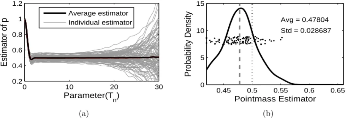
Figure 2.1: (Case 1) The left panel shows 100 simulated pointmass estimators (the gray curves), and their average (the black solid curve), as functions of Tn which is the integra-tion range parameter on the horizontal axis. In the right panel, each point is an individual pointmass estimator, and the solid curve is a kernel density estimate of these 100 estimators. The dotted and dashed vertical lines show the true value of the pointmass and the average estimator, respectively.
Figure 2.1 summarizes the performance of the pointmass estimator for 100 simulated
data sets. Figure 2.1(a) shows the change in the pointmass estimator as a function of the
integration parameter Tn of (2.4), where the vertical axis shows the value of ˆp. The gray
average of the 100 estimators. According to Figure 2.1(a), as Tn increases, the estimator
ˆ
p first decreases from 1, and increases slightly before stabilizing around the true pointmass
0.5 for Tn larger than 3. Once it stabilizes, the average estimator ˆp lies within the interval
[0.4983, 0.5010], which suggests a small bias when Tn is large enough. On the other hand,
the variance of the estimator increases asTn increases.
For Figure 2.1(b), we choose a specific value of ˆp, from each gray curve Figure 2.1(a). Since
we found that the pointmass is usually overestimated in several simulation studies, and too
largeTnresults in instability of the estimation, we choose the first local minimum of each ˆpas
our estimate, if it lies between 0 and 1. Otherwise, e.g. there is no local minimum, we choose
Tn which gives the smallest difference of ˆp, and the corresponding ˆp is used as our estimate.
Figure 2.1(b) shows the scatter plot of these 100 estimators. To show the distribution of these
estimators, their kernel density estimator (the solid curve) is plotted together. In addition,
the dotted and dashed vertical curves show the true value 0.5 and the average of the 100
estimators, respectively. For this selection method, the pointmass estimator tends to have a
slightly smaller value than the true value (the average of the 100 estimators is about 0.48).
Note that we use the same range for the horizontal axis in the corresponding panels of Figures
2.1, 2.4 and 2.7 to make the comparison clear.
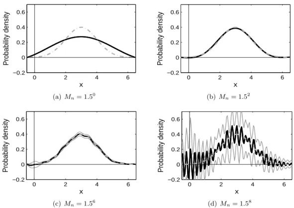
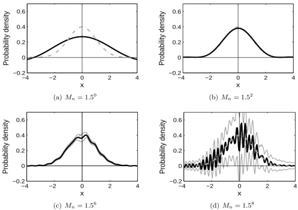
Figure 2.2 plots the density estimator in (2.6) for various values of Mn. Here, the true
value of p = 0.5 is used in estimating the density fc, in order to study the performance of
density estimation with no influence from the pointmass estimation. In each panel, the black
solid curve is the average of the estimators from the 100 samples, while the gray dash-dot
curve is the true densityfc. In addition, the gray solid curves are the average estimator ±2
standard error, which play a role as a confidence band based on the 100 samples. Note that
in some panels the curves are completely overlapping.
Similar to the pointmass estimation, a large value of the integration range parameterMn
corresponds to a small estimation bias. However, when Mn is too big, the estimator is very
wiggly, and some periodic component dominates the entire structure of the target function.
On the other hand, a small Mn gives a small estimation variance, but a large bias due to
0 2 4 6 −0.2
0 0.2 0.4 0.6
x
Probability density
(a) Mn= 1.50
0 2 4 6
−0.2 0 0.2 0.4 0.6
x
Probability density
(b)Mn= 1.52
0 2 4 6
−0.2 0 0.2 0.4 0.6
x
Probability density
(c) Mn= 1.56
0 2 4 6
−0.2 0 0.2 0.4 0.6
x
Probability density
(d)Mn= 1.58
Figure 2.2: (Case 1) Estimation of the continuous density (with known p). This plot shows the proposed estimator of fc. Each panel corresponds to the estimator based on Mn = 1.50,1.52,1.56 and 1.58. In each plot, the dash-dot curve is the true density, the black solid
curve is the average estimator, and the gray solid curves show the average estimator ± 2 standard error, based on the 100 random samples.
Interestingly, the standard error of ˆfc(x), reflected by the width of the confidence band, near
x= 0 is much larger than near x = 6. Since the normal density curve is symmetric about
its mean (3 in this case), one might expect the variations of the estimators ˆfc(0) and ˆfc(6)
would be similar, but this is not the case. The pointmass at 0 adds additional noise to the
estimation of the density function at 0. This is consistent with Remark 4, which states that
the consistency of ˆfc(x) at x=a requires more assumptions thanx6=a.
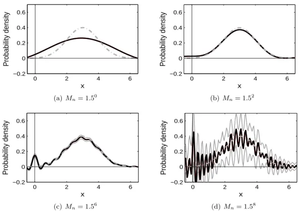
Figure 2.3 shows the density estimators which are computed using the pointmass estimator
ˆ
p, plotted in Figure 2.1(b). Compared to the density estimators obtained from the truep, the
curves in Figure 2.3 show larger values near x = 0, which is the location of the pointmass.
This result can be explained by the underestimation of the pointmasss (0.478 on average).
0 2 4 6 −0.2
0 0.2 0.4 0.6
x
Probability density
(a) Mn= 1.50
0 2 4 6
−0.2 0 0.2 0.4 0.6
x
Probability density
(b)Mn= 1.52
0 2 4 6
−0.2 0 0.2 0.4 0.6
x
Probability density
(c) Mn= 1.56
0 2 4 6
−0.2 0 0.2 0.4 0.6
x
Probability density
(d)Mn= 1.58
Figure 2.3: (Case 1) Estimation of the continuous density (with estimated ˆp). This plot shows the proposed estimator offc, based on the pointmass estimator ˆp. Each panel corresponds to the estimator based onMn= 1.50,1.52,1.56 and 1.58. In each plot, the dash-dot curve is the true density, the black solid curve is the average estimator, and the gray solid curves on the 100 random samples.
is similar to that based onp.
2.4.2 Case 2: Mixture of N(0,1) and the Pointmass
The second simulation considers the mixture of the standard normal distribution and the
pointmass at 0 with a mixing probability of 0.5. Different from the first simulation, the
location of the pointmass 0 is now the same as the mode of the standard normal distribution,
so the two components are highly overlapping. We expect the pointmassp strongly affects
the estimation offc, and ˆp is also affected byfc(x) near x= 0, which are confirmed below.
We make the same assumption about the measurement error variable Z. The sample size
and the number of iterations are also the same as the previous simulation, i.e.,n= 300 and
0 10 20 30 0.2
0.4 0.6 0.8 1 1.2
Parameter(T
n)
Estimator of p
Average estimator Individual estimator
(a)
0.45 0.5 0.55 0.6 0.65 0
5 10 15
Pointmass Estimator
Probability Density
Avg = 0.52322
Std = 0.061822
(b)
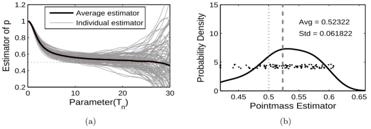
Figure 2.4: (Case 2) This plot shows the bias and variance in the estimation of the pointmass p. In the panel (a), the black solid curve shows the average estimator, and the gray curves are individual estimators. The horizontal axis Tn is the integration range parameter. The panel (b) shows a kernel density estimator of 100 pointmass estimators. The dotted vertical line shows the true value, and the dashed line shows the average estimator.
As in the previous case, in Figure 2.4(a), each gray curve shows an individual estimator
and the black solid curve is the average estimator. The overall trend of ˆp is similar to the
previous simulation, but the performance is worse as we expected: a slightly larger bias and
a much larger variance. Especially, the estimation variation is much larger when a largeTnis
used. This can be explained by the overlapping of the two mixture components. To estimate
the pointmass, we use the same criterion in choosingTn as discussed in Case 1. As shown in
Figure 2.4(b), we can see the pointmass is overestimated (the average of the 100 estimators
is around 0.52).
Similar to Figure 2.2, Figure 2.5 shows the result of the density estimation, which is based
on the true p = 0.5. One big difference from the previous simulation is the trend of the
standard error. In the current simulation, both the estimator ˆfc and the standard error are
almost symmetric about 0. In addition, the standard error has the biggest value at 0. This is
because the location of the pointmass is the center point of the continuous component. So its
effect on the estimation of fc(x) is the largest whenx = 0, and decreases as x departs from
0. Like the first case,Mn= 1.52 gives the best fit, almost overlapping the target.
We also estimatefcbased on the pointmass estimator ˆp, instead of p. As we discussed in
−4 −2 0 2 4 −0.2
0 0.2 0.4 0.6
x
Probability density
(a) Mn= 1.50
−4 −2 0 2 4
−0.2 0 0.2 0.4 0.6
x
Probability density
(b)Mn= 1.52
−4 −2 0 2 4
−0.2 0 0.2 0.4 0.6
x
Probability density
(c) Mn= 1.56
−4 −2 0 2 4
−0.2 0 0.2 0.4 0.6
x
Probability density
(d)Mn= 1.58
Figure 2.5: (Case 2) This plot shows the direct deconvolution estimator of fc. Each panel corresponds to the estimator based on M = 1.50,1.52,1.56 and 1.58. In each plot, the gray
dash-dot curve is the true density, the black solid curve is the average estimator, and the gray solid curves show the average estimator± 2 standard error.
based on the true p, except near x= 0. In opposition to Case 1, ˆfc(x) is underestimated on
the neighbor ofx= 0. It might be because that ˆp is overestimated (0.523 on average) in this
case.
In addition, we investigate the performance of the estimation of fX(x), which is our
essential estimand, in terms of the integrated squared bias, variance and mean squared error.
Figure 2.6 shows the above three numerical measures in log scale for various values of Mn.
Each panel of Figure 2.6 contains three curves. The gray dashed curve is for the case where
fX(x) is assumed to be a continuous, i.e. the pointmass component is ignored. The black
dashed curve displays the case where the truep= 0.5 is known, and hence used in estimating
fc(x). The black solid curve is used for the case where pis estimated, which fully reflects our
5 10 15 20 25 −8
−6 −4 −2 0
Mn
(a) Integrated Bias2( ˆf
X(x))
5 10 15 20 25
−8 −6 −4 −2 0
Mn
(b) Integrated Var( ˆfX(x))
5 10 15 20 25
−6 −4 −2 0 2
Mn
(c) Integrated MSE( ˆfX(x))
Figure 2.6: (Case 2) In Panels (a)-(c), the integrated squared bias, variance and mean squared error of ˆfX(x) are plotted versusMn in log-scale. In each panel, the gray dashed curve is for the case wherep= 0 is assumed when estimatingfc(x), the black dash-dot curve corresponds to the case p = 0.5, and the black solid curve shows the case where ˆp is used in estimating fc(x).
As one can expect, the performance (in terms of the mean squared error) is the best when
the true pointmassp= 0.5 is used, and the worst when the pointmass component is ignored.
When the estimated p is used, the estimation result is worse than the case p = 0.5, but is
much better than the case p= 0. In addition, when Mn is too large, all three cases perform
poorly.
2.4.3 Case 3: Mixture of Exp(1) and the Pointmass
The last simulation considers the mixture of the standard exponential distribution and the
pointmass at 0. The rest of the simulation setup is the same as the previous two cases, in
terms of the mixing probability, the measurement error distribution, the sample size, and the
number of iterations.
The difficulty in estimating the exponential density is that it has a non-smooth left
bound-ary, so the estimation would not be accurate near the left boundary (at 0). Moreover, the
location of the pointmass is near the peak of the exponential component. Like the second
case, the estimation of bothp and fc is highly related, which makes the task harder.
As shown in Figure 2.7, the pointmass is a little overestimated. The same criterion as in
0 10 20 30 0.2
0.4 0.6 0.8 1 1.2
Parameter(T
n)
Estimator of p
Average estimator Individual estimator
(a)
0.45 0.5 0.55 0.6 0.65 0
5 10 15
Pointmass Estimator
Probability Density
Avg = 0.53834
Std = 0.062403
(b)
Figure 2.7: (Case 3) This plot shows the bias and variance in the estimation of the pointmass p. In the left panel, each gray curve is an individual estimator, and the black solid curve shows the average estimator. The panel (b) shows the 100 estimators with its density. Here, the dotted/dashed lines show the true/average estimator, respectively.
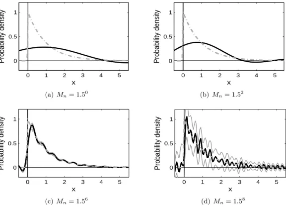
0 1 2 3 4 5
0 0.5 1
x
Probability density
(a)Mn= 1.50
0 1 2 3 4 5
0 0.5 1
x
Probability density
(b)Mn= 1.52
0 1 2 3 4 5
0 0.5 1
x
Probability density
(c) Mn= 1.56
0 1 2 3 4 5
0 0.5 1
x
Probability density
(d)Mn= 1.58
Figure 2.8: (Case 3) This plot shows the direct deconvolution estimator of fc. Each panel corresponds to the estimator based on M = 1.50,1.52,1.56 and 1.58. In each plot, the gray
second case, but slightly larger. The estimation of fc also has similar trend with the other
cases, in terms of a bias or a variance. In addition, it gives us very important information
on the boundary effect; Since the exponential density is supported only on the positive real
line, it is desirable that the estimator has only positive support. However, the support of ˆfc
includes the negative real line, and ˆfcis underestimated near 0, especially when Mnis small.
For largeMn, as shown in Figures 2.8(c) and (d), the estimator changes sharply near 0, and
oscillates on the negative real line. The variation on the negative real line can be considered as
noise in these cases, so the boundary problem is weaken. Hence a largerMnis preferred if the
target density has any bounded support. In this simulation, the density estimator performs
best when Mn= 1.56, which is much bigger than the previous two cases.
2.5
Application to the Virus-lineage Data
In this section, we illustrate the performance of the proposed estimators via an application
to the virus-lineage data in Burch et al. (2007). In this analysis, our goal is to estimate the
distribution of mutation effects on virus fitness.
2.5.1 Description on the data
For this data set, 10 virus lineages were grown in the lab for 40 days, in a manner that
promoted the accumulation of mutations in discrete random events. Plaque size was used as
a measure of viral fitness and measured everyday for each lineage.
Let Y be the reduction between two consecutive plaque size measurements. This Y is
the sum of two facts; one is the real mutation effect on plaque sizes, say X, and another
is a measurement error Z which comes from technical difficulties in measuring plaque sizes.
When the distribution ofZ is known, the distribution ofX can be estimated by the proposed
method. The relationship between two variables X and S is measured by Burch and Chao
(2004) as
X = 22.73 log(1 +S). (2.11)
not of X. It can be obtained from the relationship (2.11) and a simple change of variable
operation on the estimation results forX. Due to the scientific interest in the mutation effects
on fitness S, all the results are reported in terms ofS.
In addition, the lineages were founded with a high fitness virus to ensure that during any
given time interval, there are only two possibilities in terms of mutations:
(i) No mutation occurs, or only silent mutations occur.
(ii) A deleterious mutation occurs.
The silent mutation is defined as a mutation that has no effect on virus fitness, hence the
theoretical mutation effect X of the case (i) is 0. On the other hand, deleterious mutations
reduce the plaque sizes, so the deleterious mutation effect on plaque sizes takes only positive
values. The probability distribution of the deleterious mutation effects is usually considered
as continuous. Hence the distribution of mutation effects can be expressed as the mixture of
a point mass at 0, corresponding to case (i), and a continuous distribution (for the
deleteri-ous mutations) which is supported only on the positive real line. Unfortunately, we cannot
observe the mutation effects without measurement errors, hence it is necessary to consider
the measurement-error model on top of the mixture structure.
2.5.2 Analysis Results
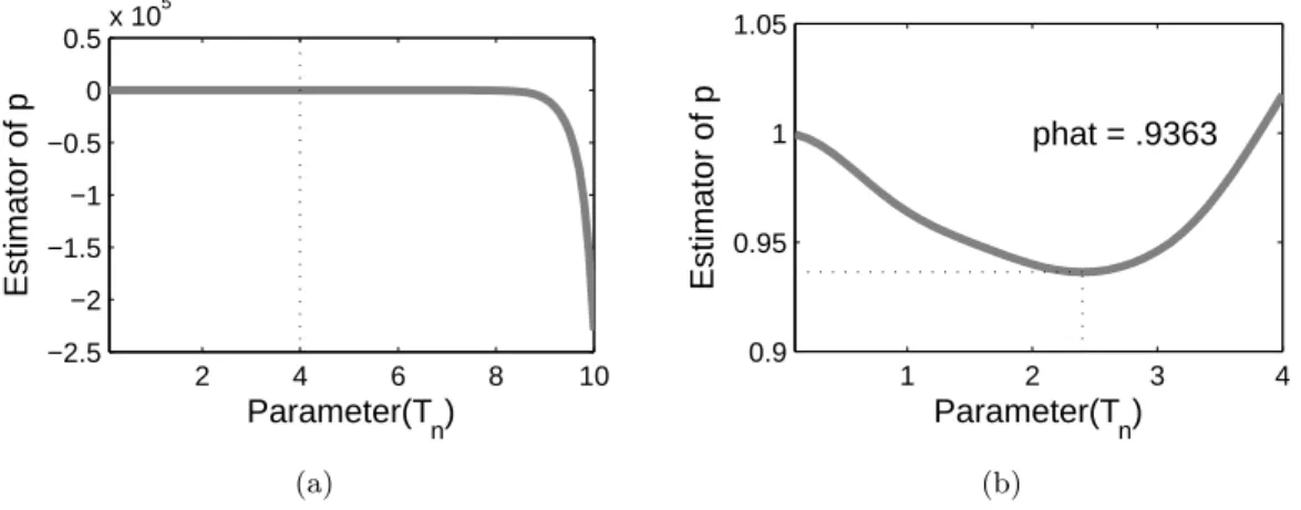
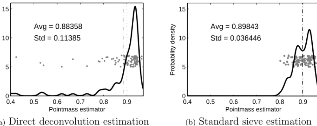
We consider the pointmass estimation result first. Figure 2.9 plots the ˆpversusTn. In Figure
2.9(a), the pointmasspis estimated forTnin the range [0.1,10]; since we assume the normality
for the measurement errorZ, the integrand of (2.4) may have very large value near tails. So
a large value of Tn results in instability of the estimation and too long computation time,
which is the reason we restrict the upper bound ofTn by 10. The estimator ˆpchanges sharply
when Tn is large, which makes it difficult to see the precise change of ˆp for small values of
Tn. So in Figure 2.9(b), the picture is zoomed into the region to the left of the vertical bar,
i.e. forTn between 0.1 and 4. From the simulation studies in Section 2.4, we have observed
addition, whenTnis large, variation of the estimation is very large. Hence we select the first
local minimum as the estimator forp, which is 0.9363 atTn= 2.4.
2 4 6 8 10
−2.5 −2 −1.5 −1 −0.5 0 0.5x 10
5
Parameter(T n)
Estimator of p
(a)
1 2 3 4
0.9 0.95 1 1.05
phat = .9363
Parameter(T
n)
Estimator of p
(b)
Figure 2.9: The panel (a) plots the estimator of the pointmass ˆp versus the range parameter Tn = (0.1, 0.2, . . . ,10). The panel (b) shows ˆp only for Tn = (0.1,0.2, . . . ,4) to get a more precise view in the region of interest. The black dotted lines highlight the suggested Tn and
ˆ p.
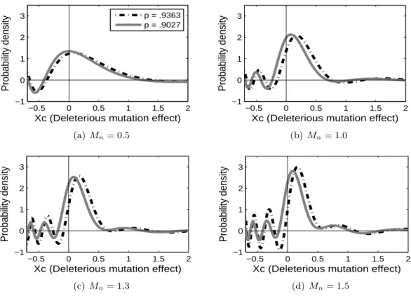
For the estimation of fc, we again use the scale space approach suggested by Chaudhuri
and Marron (2000). Figure 2.10 shows the density estimator ˆfc for different values of Mn,
the integration range parameter. Each panel shows two density curves: for the black
dash-dot curve, ˆp = 0.9363 is used, and for the gray solid curve, we use ˆp = 0.9027 which is the
pointmass estimator given by Burch et al. (2007).
When the smaller pointmass is used, the peak location of the density curve estimator is
closer to 0. It is due to the difficulty of separating small deleterious mutation effects from
silent mutation effects. If we underestimatep, the proportion of silent mutations, some silent
mutations are considered as deleterious mutations that have small effects. Except this, the
effect of pointmass estimation is small on estimating the density curve. As shown in Figure
2.10, the two curves in each panel look very similar, and the curves change in the same way
asMn changes.
We now discuss the effect of the integration range parameter. When Mn is small (for
example,Mn= 0.5), the estimator shows the overall trend of the density curve well. According
−0.5 0 0.5 1 1.5 2 −1
0 1 2 3
Xc (Deleterious mutation effect)
Probability density
p = .9363 p = .9027
(a)Mn= 0.5
−0.5 0 0.5 1 1.5 2
−1 0 1 2 3
Xc (Deleterious mutation effect)
Probability density
(b)Mn= 1.0
−0.5 0 0.5 1 1.5 2
−1 0 1 2 3
Xc (Deleterious mutation effect)
Probability density
(c)Mn= 1.3
−0.5 0 0.5 1 1.5 2
−1 0 1 2 3
Xc (Deleterious mutation effect)
Probability density
(d)Mn= 1.5
Figure 2.10: These plots show the density estimator ˆfc for different values of Mn. In each plot, the black dash-dot curve is the estimator when ˆp = 0.9363, and the gray curve is when ˆ
p= 0.9027.
the density estimator has positive values even on the negative real line, which contradicts the
fact that the deleterious mutation effects are always nonnegative. This boundary effect shows
up better whenMn is larger. In Figure 2.10(d), the density estimator changes very sharply
near 0, and oscillates on the negative real line. The variation of the density curves on the
negative part can be considered as noise, and the true underlying density curve is supported
only on the positive real line.
2.6
Theoretical Proofs
In this section, we provide technical proofs for the lemmas and theorems in Section 2.3. Note
that the estimators ˆp and ˆfc have similar structures with the density estimator of Liu and
Proof of Lemma 2.3.1 It can be seen by the simple change of variable technique. According
to the expression of ˆp,
E¡pˆ¢ = E
"
1 2TnRe
(Z Tn
−Tn
exp¡it(Y −a)¢ ϕZ(t) dt
)#
=
Z ∞
−∞
Z Tn
−Tn
1 2TnRe
(
exp¡it(y−a)¢ ϕZ(t)
)
fY(y)dt dy.
Under the assumption that ϕZ(t)6= 0, 1/ϕZ(t) is a continuous function, hence it is bounded
above on a compact set [−Tn, Tn]. In addition, |eit(y−a)| is bounded by 1. Hence the inner integrand in the above integration is absolutely integrable. So the order of integration can be
changed based on Fubini’s theorem. Then, using the definition of the characteristic function
ofY, and the relation betweenϕZ(·), ϕX(·) and ϕY(·), we have the following:
E¡pˆ¢ = 1 2Tn
Re
Z Tn
−Tn
exp(−ita)ϕX(t)dt
= 1
2Tn
Z Tn
−Tn
exp(−ita)
n
p·exp(ita) + (1−p)ϕc(t)
o
dt
= p+1−p 2Tn
Z Tn
−Tn
exp(−ita)ϕc(t)dt.
This completes the proof. ¤
Proof of Lemma 2.3.2 When a random variable is symmetric about 0, its characteristic
function is a real valued function, and symmetric about 0. So ϕZ(·) is a real valued even
function. Then we can get
Var¡pˆ¢ = 1 4nT2
n Var
µZ Tn
−Tn
cost(Y −a) ϕZ(t) dt
= 1
nT2
n E
µZ Tn
0
costV −E(costV)
ϕZ(t) dt
¶2
,
that cos(·) is also an even function. Recall the cosine product formula that 2 cosAcosB =
cos(A+B) + cos(A−B). Then the above equation becomes
Var¡pˆ¢ = 1 2nT2
n
Z Tn
0 Z Tn
0
E©cos(s+t)V + cos(s−t)Vª−2E(cossV)E(costV)
ϕZ(s)ϕZ(t) ds dt
= 1
2nT2
n
Z Tn
0 Z Tn
0
Re©ϕV(s+t) +ϕV(s−t)
ª
−2Re©ϕV(s)
ª
Re©ϕV(t)
ª
ϕZ(s)ϕZ(t) ds dt.
This completes the proof. ¤
Proof of Theorem 2.3.3 To show the consistency, we will show that both the bias and the
variance of ˆpconverges to 0. From Lemma 2.3.1,
bias¡pˆ¢ = 1−p 2Tn
Z Tn
−Tn
exp(−ita)ϕc(t)dt
= (1−p)π
Tn ·
1 2π
Z Tn
−Tn
exp(−ita)ϕc(t)dt.
Clearly (1−p)π/Tnconverges to 0, and the latter part converges tofc(a) becauseϕc(t) is a
characteristic function of a continuous random variableXc. Therefore the bias of ˆpconverges
to 0 asn→ ∞.
Since |ϕV(t)| ≤1 for any t,
¯
¯Re{ϕV(s+t) +ϕV(s−t)} −2Re ϕV(s)Re ϕV(t)¯¯≤4.
Then the variance of ˆp is bounded by
Var¡pˆ¢≤ 2
nT2
n
Z Tn
0
Z Tn
0
1
ϕZ(s)ϕZ(t)ds dt= 2
µ
1 n1/2T
n
Z Tn
0
1 ϕZ(t)dt
¶2
. (2.12)
Proof of Theorem 2.3.4 First, we divide ˆfc(x) into three parts:
ˆ
fc(x) = 1
2π(1−p)ˆ
Z Mn
−Mn
Re 1 n n X j=1
exp¡it(Yj−x)
¢
ϕZ(t)
−pˆ·exp¡it(a−x)¢
dt
= 1−p 1−pˆ
"
Re 2π(1−p)
Z Mn
−Mn ½ 1 n n X j=1
exp¡it(Yj−x)
¢
ϕZ(t) −p·exp
¡
it(a−x)¢
¾
dt
+ Re
2π(1−p)
Z Mn
−Mn
(p−p) expˆ ¡it(a−x)¢dt
#
= T1(T2+T3),
where
T1 = 1−pˆ 1−p,
T2 = 2π(11−p)Re Z Mn
−Mn ½ 1 n n X j=1
exp¡it(Yj−x)
¢
ϕZ(t) −p·exp
¡
it(a−x)¢
¾
dt,
and T3 = 2π(11−p)Re Z Mn
−Mn
(p−p) expˆ ¡it(a−x)¢dt.
To show the consistency of ˆfc(x), we will show that T1 → 1, T2 → fc(x) and T3 → 0 in
probability, asngoes to infinity.
Since ˆp converges to p in probability by Theorem 2.3.3, T1 converges to 1 in probability.
It is because ˆpis a consistent estimator of pand f(x) = 1/(1−x) is a continuous function of
x except the casex= 1.
Now we show T3 converges to 0. Since we only consider the case x6=a,
T3 = 2π(11−p) ¡
p−pˆ¢·Re
Z Mn
−Mn
eit(a−x)dt (2.13)
= p−pˆ 2π(1−p)
Z Mn
−Mn
cost(a−x)dt= (p−p) sinˆ Mn(a−x)
π(1−p)(a−x) . (2.14)
Here,|sinMn(a−x)|is uniformly bounded by 1, and we already showed ˆpconverges top, i.e.
ˆ
p−p converges to 0 in probability. HenceT3 converges to 0 in probability.
to show that E(T2) → fc(x), and Var(T2) → 0 as n goes to infinity. From the definition of
T2,
E(T2) = 2π(11−p)Re Z ∞
−∞
Z Mn
−Mn ½
exp¡it(y−x)¢
ϕZ(x) −p·exp
¡
it(a−x)¢
¾
fY(y)dt dy.
Since ϕZ(t) 6= 0 for any t, the absolute value of the above integrand is bounded by an
integrable function, i.e.
¯ ¯ ¯ ¯ ¯
exp¡it(y−x)¢
ϕZ(x) −p·exp
¡
it(a−x)¢
¯ ¯ ¯ ¯
¯fY(y)≤ ï
¯ ¯ ¯ϕ 1
Z(x)
¯ ¯ ¯ ¯+p
!
fY(y).
Then, by Fubini’s theorem,E(T2) is rewritten as
E(T2) = 2π(11−p)Re Z Mn
−Mn ½
ϕY(t) exp(−itx)
ϕZ(t) −p·exp
¡
it(a−x)¢
¾
dt
= 1
2π(1−p)Re
Z Mn
−Mn n
ϕX(t)−p·exp(ita)
o
exp(−itx)dt.
= 1
2πRe
Z Mn
−Mn
ϕc(t) exp(−itx)dt.
The last equality comes from (2.5). SinceMn goes to infinity asnincreases,
E(T2)→Re
µ
1 2π
Z ∞
−∞
ϕc(t) exp(−itx)dt
=Re
³
fc(x)
´
=fc(x),
asngoes to infinity.
The next part shows the calculation of the variance of T2, which is very similar to the
computation of Var(ˆp) in the proof of Lemma 2.3.2.
Var(T2) = Var
1
2nπ(1−p) n
X
j=1 Z Mn
−Mn ½
cost(Yj−x)
ϕZ(t) −p·exp
¡
it(a−x)¢
¾ dt = Var 1
2nπ(1−p) n
X
j=1 Z Mn
−Mn
cost(Yj−x) ϕZ(t) dt