i
Computational Complexity: A Modern
Approach
Draft of a book: Dated January 2007
Comments welcome!
Sanjeev Arora and Boaz Barak
Princeton UniversityNot to be reproduced or distributed without the authors’ permission
This is an Internet draft. Some chapters are more finished than others. References and attributions are very preliminary and we apologize in advance for any omissions (but hope you
will nevertheless point them out to us).
Please send us bugs, typos, missing references or general comments to
Chapter 9
Cryptography
“Human ingenuity cannot concoct a cipher which human ingenuity cannot resolve.”
E. A. Poe, 1841
“In designing a good cipher ... it is not enough merely to be sure none of the standard methods of cryptanalysis work– we must be sure that no method whatever will break the system easily. This, in fact, has been the weakness of many systems. ... The problem of good cipher design is essentially one of finding difficult problems, subject to certain other conditions. This is a rather unusual situation, since one is ordinarily seeking the simple and easily soluble problems in a field.”
C. Shannon [Sha49]
“While the NPcomplete problems show promise for cryptographic use, current un-derstanding of their difficulty includes only worst case analysis. For cryptographic purposes, typical computational costs must be considered.”
W. Diffie and M. Hellman [DH76]
Cryptography is much older than computational complexity— ever since people began to write, they were some things they wanted to keep secret, and so numerous methods ofencryptionor “secret writing” have been devised over the years. All these methods had one common characteristic— sooner or later they were broken. But everything changed in 1970’s, when the works of several researchers, modern cryptography was born. In modern cryptography, the security of encryption schemes no longer depended on complicated and secret encryption methods. Rather, modern cryptographic schemes rely for their security on the computational hardness of simple publicly-known and well studied computational problems. We relate these problems to the security of our schemes by means of reductions similar (though not identical) to those used in the theory of
NP-completeness.
This new focus on building system from basic problems via reductions enabled modern cryp-tography to achieve two seemingly contradictory goals. On the one hand these new schemes are much more secure— systems such as the RSA encryption [RSA78] have withstood more attacks by talented mathematicians assisted with state of the art computers than every previous encryption in history, and yet still remain unbroken. On the other hand, their security requirements are much more stringent— we require the schemes to remain secure even when the encryption key is known to the attacker (i.e., public key encryption), and even when the attacker gets access to encryptions and decryptions of her choice (so calledchosen plaintext andchosen ciphertext attacks). Moreover, modern cryptography provides schemes that go much beyond simple encryption— tools such as digital signatures, zero knowledge proofs, electronic voting and auctions, and more. All of these are shown to be secure againstevery polynomial-time attack, and not just attacks we can think of today, as long as the underlying computational problem is indeed hard.
p9.2 (160) 9.1. PERFECT SECRECY AND ITS LIMITATIONS Research on modern cryptography led to significant insights that had impact and applications in complexity theory and beyond that. One is the notion ofpseudorandomness. Philosophers and scientists have struggled for years to define what is a “random enough” string. Cryptography’s answer to this question is that it suffices if this string is drawn from a distribution that “looks random” to allefficient (i.e., polynomial-time) observers (see Section 9.2.3). This notion is crucial for the construction of many cryptographic schemes, but is also extremely useful in other areas where random bits are needed. For example cryptographic pseudorandom generators can be used to reduce the randomness requirements of probabilistic algorithms such as the ones we saw in Chapter 7; see also Chapter 20. Another insight is the notion of simulation. A natural question in cryptography is how do you demonstrate that an attacker cannot learn anything about some secret information from observing the behavior of parties holding this information. Cryptography’s answer is to show that the attacker’s observations can besimulated without any access to the secret information. This is epitomized in the notion of zero knowledge proofs covered in Section 9.4, but is used in many other cryptographic applications.
We start the chapter in Section 9.1 with Shannon’s definition of perfectly secret encryption and the limitations of such systems. These limitations lead us to consider encryptions that are only computationally secret— secure for polynomial-time eavesdroppers— which we construct in Section 9.2 usingpseudorandom generators. Then, in Section 9.2.3 we show how these generators can be constructed from weaker assumptions. In Section 9.4 we describe zero knowledge proofs, a fascinating concept that has had deep implications for cryptography and complexity alike. Finally, in Section 9.5 we mention how these concepts can be used to achieve security in a variety of settings. Cryptography is a huge topic, and so naturally this chapter covers only a tiny sliver of it; the chapter notes contain some excellent choices for further reading. Cryptography is intimately related to notions such as average-case complexity, hardness amplifications and derandomization, see chapters 18, 19, and 20.
9.1
Perfect secrecy and its limitations
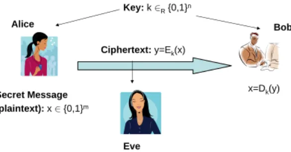
Secret Message (plaintext):x ∈{0,1}m Key:k ∈R{0,1}n Alice Bob Ciphertext:y=Ek(x) Eve x=Dk(y)
Figure 9.1: In a private key encryption, Alice and Bob share a secret keykchosen at random. To send a plaintext messagexto Bob, Alice sendsy=Ek(x) whereE(·) is theencryption function that takes a keykand plaintextxto
compute the ciphertexty. Bob can decodexby running the decryption algorithmDon inputsk, y.
The fundamental task of cryptography is encryption. The basic setting is described in Fig-ure 9.1— Alice wants to send a secret message x (known as the plaintext) to Bob, but her ad-versary Eve is eavesdropping to the communication channel between Alice and Bob. Thus Alice will “scramble” the plaintextxusing anencryption algorithm Eto obtain aciphertext y which she sends to Bob. Presumably it will be hard or even impossible for Eve to decode the plaintextxfrom the ciphertexty, but Bob will be able to do so using the decryption algorithm D. Of course to do so Bob has to know something that Eve doesn’t. In the simple setting of private key encryption we assume that Alice and Bob share some secret stringk(known as thekey) that is chosen at ran-dom. (Presumably, Alice and Bob met beforehand and agreed on the keyk.) Thus, the encryption scheme is composed of a pair of algorithms (E,D) each taking a key and a message (where we write
9.2. COMPUTATIONAL SECURITY, ONE-WAY FUNCTIONS, AND PSEUDORANDOM
GENERATORS p9.3 (161)
the key input as a subscript), such that for every keyk and plaintext x
Dk(Ek(x)) =x . (1)
The condition (1) says nothing about the security of the scheme, and could be satisfied by the trivial “encryption” that just outputs the plaintext message. It turns out that defining security is quite subtle. A first attempt at a definition might be to say that a scheme is secure if Eve cannot computexfromEk(x), but this may not be sufficient, because this does not rule out the possibility
of Eve computing some partial information on x. For example, if Eve knows that the plaintext is either the message “buy” or “sell” then it will be enough for her to learn only the first character of the message, even if she can’t recover it completely. Shannon gave the following definition of secure private key encryption that ensures Eve does not learn anything about the plaintext from the ciphertext:
Definition 9.1 (Perfect Secrecy)
Let (E,D) be an encryption scheme for messages of lengthmand with a key of lengthnsatisfying (1). We say that (E,D) isperfectly secret if for every pair of messagesx, x0 ∈ {0,1}m, the distributions
EUn(x) and EUn(x
0) are identical. (Recall thatU
ndenotes the uniform distribution over{0,1}n.)
In a perfectly secret encryption, the ciphertext that Eve sees always has the same distribution, regardless of the plaintext, and so Eve gets absolutely no information on the plaintext. It might seem like a condition so strong that it’s impossible to satisfy, but in fact there’s a very simple perfectly secret encryption scheme. In theone-time pad scheme, to encrypt a messagex∈ {0,1}n
we choose a random key k ∈R {0,1}n and encrypt x by simply sending x⊕k (⊕ denotes bitwise XOR). The receiver can recover the message x from y = x⊕k by XOR’ing y once again with k. It’s not hard to see that the ciphertext is distributed uniformly regardless of the plaintext message encrypted, and hence the one-time pad is perfectly secret (see Exercise 9.1).
The name “one-time pad” is akin to calling a rifle the “point-away gun”— if you are tempted to ignore the name and reuse the same key for two different messages, then the results for security could be disastrous. In fact, it turns out there is no perfectly secret encryption scheme that uses key size shorter than the message size (see Exercise 9.2).
9.2
Computational security, one-way functions, and
pseudoran-dom generators
In today’s applications people want to exchange securely megabytes or even gigabytes of informa-tion, while using secret keys that are at most a few hundred of bits long. But we already saw this is impossible to achieve with perfect secrecy. We can bypass this obstacle by relaxing the perfect secrecy condition to consider only adversaries that areefficient (i.e., run in polynomial-time). The question of whether this relaxation enables reducing the key size turns out to be closely connected to the problem of Pvs. NP:
Lemma 9.2 Suppose that P = NP. Let (E,D) be any polynomial-time computable encryption scheme satisfying (1) with key shorter than the message. Then, there is a polynomial-time algorithm A satisfying that for every input lengthm, there is a pair of messages x0, x1 ∈ {0,1}m such that
Pr
b∈R{0,1}
k∈R{0,1}
n
[A(Ek(xb)) =b]≥3/4, (2)
p9.4 (162)
9.2. COMPUTATIONAL SECURITY, ONE-WAY FUNCTIONS, AND PSEUDORANDOM GENERATORS Such an algorithm completely breaks the security of the encryption scheme since, as demon-strated by the “buy”/“sell” example of Section 9.1, a minimal requirement from an encryption is that Eve cannot tell which one of two random messages was encrypted with probability much better than 1/2.
Proof of Lemma 9.2: Let (E,D) be an encryption for messages of lengthmand with key length n < m as in the lemma’s statement. Let S ⊆ {0,1}∗ denote the support of EUn(0
m). Note that
y ∈ S if and only if y =Ek(0m) for some k, and hence ifP =NP then membership in S can be
efficiently verified. Our algorithmA will be very simple— on input y, it outputs 0 if y∈S, and 1 otherwise. We claim that settingx0= 0m, there exists somex1 ∈ {0,1}m such that (2) holds.
Indeed, for every message x, letDx denote the distribution EUn(x). By the definition of A and
the fact that x0 = 0m, Pr[A(Dx0) = 0] = 1. Because
Pr
b∈R{0,1} k∈R{0,1}
n
[A(Ek(xb)) =b] = 1/2Pr[A(Dx0) = 0]+1/2Pr[A(Dx1) = 1] =1/2+1/2Pr[A(Dx1) = 1],
it suffices to show that there’s some x1 ∈ {0,1}m such that Pr[A(Dx1) = 1] ≥1/2. In other words,
it suffices to show that Pr[Dx1 ∈S]≤1/2 for somex1 ∈ {0,1}
m
.
Suppose otherwise that Pr[Dx ∈ S] > 1/2 for every x ∈ {0,1}m. Define S(x, k) to be 1
if Ek(x) ∈ S and to be 0 otherwise, and let T = Ex∈R{0,1}
m,k∈{0,1}n[S(x, k)]. Then under our
assumption,T >1/2. But reversing the order of expectations, we see that
T = E k∈{0,1}n E x∈{0,1}m[S(x, k)] ≤1/2,
where the last inequality follows from the fact that for every fixed key k, the map x 7→ Ek(x) is
one-to-one and hence at most 2n≤2m/2 of thex’s can be mapped under it to a setS of size≤2n.
Thus we obtained a contradiction to the assumption that Pr[Dx ∈S]>1/2 for every x∈ {0,1}m.
Since we don’t have a proof that P6=NP, Lemma 9.2 means that we cannot construct encryp-tions that areunconditionally proven to be secure against polynomial-time eavesdroppers. But we might be able to construct such schemes under certain conjectures such as P 6= NP. We don’t know how to do so under the conjecture that P6=NP, but can use a certain stronger conjecture. Call a function µ :N → [0,1] negligible if (n) = n−ω(1) (i.e., for every c and sufficiently large n,
(n)< n−c). Because negligible functions tend to zero very fast as their input grows, events that happen with negligible probability can be safely ignored in most practical and theoretical settings. A one-way function is a function that is easy to compute but hard to invert:
Definition 9.3 (One way functions)
A polynomial-time computable functionf :{0,1}∗ → {0,1}∗ is aone-way function
if for every probabilistic polynomial-time algorithmA there is a negligible function
:N→[0,1] such that for everyn,
Pr x∈R{0,1} n y=f(x) [A(y) =x0 s.t. f(x0) =y]< (n). Conjecture 9.4
There exists a one-way function.
Exercise 9.5 asks you to show that Conjecture 9.4 implies that P 6= NP. Most researchers believe Conjecture 9.4 is true because there are several examples for functions that no one has yet been able to invert.
9.2. COMPUTATIONAL SECURITY, ONE-WAY FUNCTIONS, AND PSEUDORANDOM
GENERATORS p9.5 (163)
9.2.1 Examples for one way functions
Here are some examples for functions that are conjectured to be one way. (Of course, until we prove that P6=NPwe’ll not be able to prove that any of these is in fact a one-way function.)
Multiplication Simple multiplication turns out to be hard to invert. That is, the function that treats its input x∈ {0,1}n as describing twon/2-bit numbersA and B and outputsA·B is believed to be one way. Inverting this function is known as theinteger factorization problem. Of course, it’s easy to factor a numberN using N (or even only√N) trial divisions. But if
N is an n-bit number this is an exponential in n number of operations. At the moment no polynomial (i.e., polylog(N)) time algorithm is known for this problem, and the best factoring algorithm runs in time 2O(log1/3N
√
log logN) [LLMP90].1
A more standard implementation of a one-way function based on factoring is the following. Treat the input x ∈ {0,1}n as randomness that is used to generate two random n1/3-bit primes P and Q. (We can do so by generating random numbers and testing their primality using the algorithm described in Chapter 7.) We then outputP ·Q.
Factoring integers has captured the attention of mathematicians for at least two millennia, way before computers were invented. Because despite all this study, no efficient factorization algorithm was found, many people conjecture that no such algorithm exists and this function is indeed a one-way function, though this conjecture is not as a strongly supported as the conjecture thatP6=NPor the conjecture thatsome one-way function exists.
RSA and Rabin functions (These examples require a bit of number theory; see Section A.4 for a quick review) TheRSA function2 is another very popular candidate for a one-way function. We assume that for every input length n there is an n-bit composite integer N that was generated in some way, and some number e that is coprime to ϕ(N) = |Z∗N| where Z∗N is
the multiplicative group of numbers coprime to N. (Typically N would be generated as a product of two n/2-long primes; eis often set to be simply 3.) The functionRSAN,e treats
its input as a numberX inZ∗N and outputs Xe (mod N).3 It can be shown that becausee
is coprime toϕ(N), this function is one-to-one on ZN∗. A related candidate one-way function is the Rabin function that given a number N that is the product of two odd primes P, Q
such that P, Q = 1 (mod 4), maps X ∈ QRN into X2 (modN), where QRN is the set of
quadratic residuesmoduloN (an elementX∈Z∗N is a quadratic residue moduloN ifX=W2
(modN) for someW ∈Z∗
N). Again, it can be shown that this function is one-to-one onQRN.
While both the RSA function and the Rabin function are believed to be hard to invert, inverting them is actually easy if one knows the factorization of N. In the case of the RSA function, the factorization can be used to compute ϕ(N) and from that the number d such that d = e−1 (modϕ(N)). It’s not hard to verify that the function Yd (modN) is the inverse of the function Xe (modN). In the case of the Rabin function, if we know the factorization then we can use the Chinese Remainder Theorem to reduce the problem of taking a square root moduloN to taking square roots modulo the prime factors of N, which can be done in polynomial time. Because these functions are conjectured hard to invert but become easy to invert once you know certain information (i.e., N’s factorization), they are known as trapdoor one-way functions, and are crucial to obtaining public key cryptography.
1IfAandB are chosen randomly then it’s not hard to find asome prime factor ofA·B, sinceA·B will have a
small prime factors with high probability. But finding the all the prime factors or even finding any representation of A·Bas the multiplication of two numbers each no larger than 2n/2 can be shown to be equivalent (up to polynomial
factor) to factoring the product of two random primes.
2RSA are the initials of this function’s discoverers; see the chapter notes. 3
We can map the input toZ∗N by simply reducing the input moduloN— the probability (over the choice of the
p9.6 (164)
9.2. COMPUTATIONAL SECURITY, ONE-WAY FUNCTIONS, AND PSEUDORANDOM GENERATORS It it known that inverting Rabin’s function is in fact computationally equivalent to factoring
N (see Exercise 9.7). No such equivalence is known for the RSA function.
Levin’s universal one-way function There is a function fU that has a curious property: if there existssome one-way functionf thenfU is also a one-way function. For this reason, the function fU is called a universal one-way function. It is defined as follows: treat the input as a list x1, . . . , xlogn of n/logn bit long strings. Output Mn
2
1 (x1), . . . , Mn
2
logn(xn) where
Mi denotes theith Turing machine according to some canonical representation and we define
Mt(x) to be the output of the Turing machineM on inputxifMuses at mosttcomputational steps on inputx. IfM uses more than t computational steps on x then we define Mt(x) to be the all-zeroes string 0|x|. Exercise 9.6 asks you to prove the universality offU.
There are also examples of candidate one-way functions that have nothing to do with number theory (e.g., one-way functions arising from block ciphers such as the AES [DR02]).
9.2.2 Encryption from one-way functions
If Conjecture 9.4 is true then there do exist secure encryption schemes with keys much shorter than the message length:
Theorem 9.5 (Encryption from one-way function)
Suppose that one-way functions exist. Then for everyc∈Nthere exists a computa-tionally secure encryption scheme(E,D)usingn-length keys fornc-length messages.
Of course to make sense of Theorem 9.5, we need to define the term “computationally secure”. The idea is to follow the intuition that a secure encryption should not reveal any partial information about the plaintext to a polynomial-time eavesdropper, but due to some subtleties, the actual definition is somewhat cumbersome. Thus, for the sake of presentation we’ll use a simpler relaxed definition that an encryption is “computationally secure” if any individual bit of the plaintext chosen at random cannot be guessed by the eavesdropper with probability non-negligibly higher than 1/2. That is, we say that a scheme (E,D) using length n keys for length m messages is
computationally secure if for every probabilistic polynomial-time A, there’s a negligible function
:N→[0,1] such that Pr k∈R{0,1} n x∈R{0,1} m [A(Ek(x)) = (i, b) s.t. xi=b]≤1/2+(n). (3)
The full-fledged, stronger notion of computational security (whose standard name is semantic se-curity) is developed in Exercise 9.9, where it is also shown that Theorem 9.5 holds also for this stronger notion.
9.2.3 Pseudorandom generators
The idea behind the proof of Theorem 9.5 can be summarized as follows. We already have an encryption scheme to encrypt lengthmmessages using a lengthmrandom key— the one-time pad. We will show that it’s possible to generate this key using only nm random bits, in a way such that security will still hold with respect to polynomial-time eavesdroppers. It turns out that if one-way functions exist then there is a very general tool that allows us to expand a short random string into a much longer string that is still sufficiently “random looking” for all practical purposes. This tool is called apseudorandom generator, and as you can imagine, has many applications even beyond cryptography.
9.3. PSEUDORANDOM GENERATORS FROM ONE-WAY PERMUTATIONS p9.7 (165)
Example 9.6
What is a random-enough string? Here is Kolmogorov’s definition: A string of length nis random if no Turing machine whose description length is<0.99n(say) outputs this string when started on an empty tape. This definition is the “right” definition in some philosophical and technical sense (which we will not get into here) but is not very useful in the complexity setting because checking if a string is random according to this definition is undecidable.
Statisticians have also attempted definitions which boil down to checking if the string has the “right number” of patterns that one would expect by the laws of statistics, e.g. the number of times 11100 appears as a substring. (See [Knu73] for a comprehensive discussion.) It turns out that such definitions are too weak in the cryptographic setting: one can find a distribution that passes these statistical tests but still will be completely insecure if used to generate the pad for the one-time pad encryption scheme.
Cryptography’s answer to the above question is simple and satisfying— a distribution is pseu-dorandom if it cannot be distinguished from the uniform distribution by any polynomial-time algorithm:
Definition 9.7 (Secure pseudorandom generators)
LetG:{0,1}∗→ {0,1}∗ be a polynomial-time computable function. Let`:N→N
be a polynomial-time computable function such that `(n) > n for every n. We say that G is a secure pseudorandom generator of stretch `(n), if |G(x)| = `(|x|) for every x ∈ {0,1}∗ and for every probabilistic polynomial-time A, there exists a negligible function :N→[0,1] such that
Pr[A(G(Un)) = 1]−Pr[A(U`(n)) = 1] < (n), for everyn∈N.
Theorem 9.8 (Pseudorandom generators from one-way functions)
If one-way functions exist, then for everyc∈N, there exists a secure pseudorandom generator with stretch`(n) =nc.
Definition 9.7 states that it’s infeasible for polynomial-time adversaries to distinguish between a completely random string of length`(n) and a string that was generated by applying the generator
G to a much shorter random string of length n. Thus, it’s not hard to verify that Theorem 9.8 implies Theorem 9.5: if we modify the one-time pad encryption to generate its nc-length random key by applying a secure pseudorandom generator with stretch nc to a shorter key of length n,
then a polynomial-time eavesdropper would not be able to tell the difference. Specifically, if there was an adversary Athat can predict a bit of the plaintext with probability noticeably larger than
1/2, thus violating the computational security requirement (3), then because such prediction is
impossible when the key is truly random (see Exercise 9.3),A can be used to distinguish between a pseudorandom and truly random key, thus contradicting the security of the generator as per Definition 9.7.
9.3
Pseudorandom generators from one-way permutations
p9.8 (166) 9.3. PSEUDORANDOM GENERATORS FROM ONE-WAY PERMUTATIONS
Lemma 9.9 Suppose that there exists a one-way functionf :{0,1}∗ → {0,1}∗such thatf is one-to-one for every x∈ {0,1}∗, |f(x)|=|x|. Then, for everyc∈N, there exists a secure pseudorandom generator with stretchnc.
The proof of Lemma 9.9 does demonstrate some of the ideas behind the proof of the more general Theorem 9.8. Moreover, these ideas are of independent interest and have found several applications in other areas of Computer Science.
9.3.1 Unpredictability implies pseudorandomness
The following alternative characterization of pseudorandom generators will be useful to prove Lemma 9.9. Let G : {0,1}∗ → {0,1}∗ be a polynomial-time computable function with stretch
`(n) (i.e., |G(x)|=`(|x|) for every x∈ {0,1}∗). We call G unpredictable if for every probabilistic polynomial-time B there is a negligible function:N→[0,1] such that
Pr x∈R{0,1} n y=G(x) i∈R[`(n)] [B(1n, y1, . . . , yi−1) =yi]≤1/2+(n). (4)
Clearly, ifGis a pseudorandom generator then it is also unpredictable. Indeed, ify1, . . . , y`(n) were
uniformly chosen bits then it would be impossible to predictyi giveny1, . . . , yi−1, and hence if such
a predictor exists when y =G(x) for a random x, then the predictor can distinguish between the distributionU`(n) and G(Un). Interestingly, the converse direction also holds:
Theorem 9.10 (Unpredictability implies pseudorandomness [Yao82b])
Let ` :N → N be some polynomial-time computable function, and G : {0,1}∗ →
{0,1}∗ be a polynomial-time computable function such that |G(x)| = `(|x|) for every x ∈ {0,1}∗. If G is unpredictable then it is a secure pseudorandom gen-erator. Moreover, for every probabilistic polynomial-time algorithm A, there ex-ists a probabilistic polynomial-time B such that for every n ∈ N and > 0, if
Pr[A(G(Un)) = 1]−Pr[A(U`(n)) = 1]≥, then Pr x∈R{0,1} n y=G(x) i∈R[`(n)] [B(1n, y1, . . . , yi−1) =yi]≥1/2+/`(n)
Proof: First, note that the main result does follow from the “moreover” part. Indeed, suppose
thatGis not a pseudorandom generator and hence there is some algorithmA and constantc such that
Pr[A(G(Un)) = 1]−Pr[A(U`(n)) = 1]
≥n−c (5)
for infinitely many n’s. Then we can ensure (perhaps by changingA to the algorithm 1−A), that for infinitely manyn’s, (5) holds without the absolute value. For every suchn, we’ll get a predictor
B that succeeds with probability1/2+n−c/`(n), contradicting the unpredictability property.
We turn now to proving this “moreover” part. Let A be some probabilistic polynomial-time algorithm that is supposedly more likely to output 1 on input from the distribution G(Un)
than on input from U`(n). Our algorithm B will be quite simple: on input 1n, i ∈ [`(n)] and
y1, . . . , yi−1, Algorithm B will choose zi, . . . , x`(n) independently at random, and compute a =
A(y1, . . . , yi−1, zi, . . . , z`(n)). If a = 1 then B surmises its guess for zi is correct and outputs zi;
9.3. PSEUDORANDOM GENERATORS FROM ONE-WAY PERMUTATIONS p9.9 (167) Letn∈Nand `=`(n) and suppose that Pr[A(G(Un)) = 1]−Pr[A(U`(n)) = 1]≥. We’ll show
that Pr x∈R{0,1} n y=G(x) i∈R[`] [B(1n, y1, . . . , yi−1) =yi]≥1/2+/` . (6)
To analyze B’s performance, we define the following ` distributions D0, . . . ,D` over {0,1}`. For
every i, the distribution Di is obtained as follows: choose x ∈R {0,1} n
and let y = G(x), output
y1, . . . , yi, zi+1, . . . , z`, where zi+1, . . . , z` are chosen independently at random in {0,1}. Note that
D0=U`whileD`=G(Un). For everyi∈ {0, .., `}, definepi= Pr[A(Di) = 1]. Note thatp`−p0 ≥.
Thus, writing
p`−p0 = (p`−p`−1) + (p`−1−p`−2) +· · ·+ (p1−p0),
we get that P`
i=1(pi−pi−1) ≥ or in other words, Ei∈[`][pi −pi−1] ≥ /`. We will prove (6) by
showing that for everyi, Pr
x∈R{0,1} n y=G(x)
[B(1n, y1, . . . , yi−1) =yi]≥1/2+ (pi−pi−1).
Recall that B makes a guess zi for yi and invokes A to obtain a value a, and then outputs zi if
a= 1 and 1−zi otherwise. Thus B predictsyi correctly if either a= 1 and yi =zi ora6= 1 and
yi = 1−zi, meaning that the probability this event happens is
1/2Pr[a= 1|zi=yi] +1/2(1−Pr[a= 1|zi= 1−yi]). (7)
Yet, one can verify that conditioned on zi = yi, B invokes A with the distribution Di, meaning
that Pr[a= 1|zi =yi] =pi. On the other hand if we don’t condition on zi then the distribution B
invokes A is equal toDi−1. Hence,
pi−1 = Pr[a= 1] =1/2Pr[a= 1|zi =yi] +1/2Pr[a= 1|zi = 1−yi] =1/2pi+1/2Pr[a= 1|zi = 1−yi].
Plugging this into (7) we get that B predictsyi with probability 1/2+pi−pi−1.
9.3.2 Proof of Lemma 9.9: The Goldreich-Levin Theorem
Let f be some one-way permutation. To prove Lemma 9.9 we need to use f to come up with a pseudorandom generator with arbitrarily large polynomial stretch `(n). It turns out that the crucial step is obtaining a pseudorandom generator that extends its input by one bit (i.e., has stretch`(n) =n+ 1).This is achieved by the following theorem:
Theorem 9.11 (Goldreich-Levin Theorem [GL89])
Suppose that f : {0,1}∗ → {0,1} is a one-way function such that f is one-to-one and|f(x)|=|x|for everyx∈ {0,1}∗. Then, for every probabilistic polynomial-time algorithm Athere is a negligible function :N→[0,1]such that
Pr
x,r∈R{0,1}n
[A(f(x), r) =xr]≤1/2+(n),
wherexr is defined to bePni=1xiri (mod 2).
Theorem 9.11 immediately implies that the function G(x, r) =f(x), r, xr is a secure pseu-dorandom generator that extends its input by one bit (mapping 2n bits into 2n+ 1 bits). Indeed, otherwise by Theorem 9.10 there would be a predictor B for this function. But because f is a
p9.10 (168) 9.3. PSEUDORANDOM GENERATORS FROM ONE-WAY PERMUTATIONS permutation over{0,1}n, the first 2nbits ofG(U2n) are completely random and independent, and
hence cannot be predicted from their predecessors with probability better than 1/2. This means
that a predictor for this function would have to have noticeably larger than1/2success of predicting
the 2n+ 1th bit from the previous 2nbits, which exactly amounts to violating Theorem 9.11.
Proof of Theorem 9.11: Suppose, for the sake of contradiction, that there is some
proba-bilistic polynomial-time algorithmAthat violates the theorem’s statement. We’ll use A to show a probabilistic polynomial-time algorithm B that inverts the permutationf, in contradiction to the assumption that it is one way. Specifically, we will show that if for some n,
Pr
x,r∈R{0,1}
n[A(f(x), r) =xr]≥
1/2+ , (8)
thenB will run inO(n2/2) time and invert the one-way permutationf on inputs of lengthnwith probability at least Ω(). This means that if A’s success probability is more than 1/2+n−c for
some constantc and infinitely manyn’s, then B runs in polynomial-time and inverts the one-way permutation with probability at least Ω(n−c) for infinitely manyn’s.
Let n, be such that (8) holds. Then by a simple averaging argument, for at least an /2 fraction of the x’s, the probability over r that A(f(x), r) = xr is at least 1/2+/2. We’ll call
such x’s good, and show an algorithmB that with high probability invertsf(x) for every goodx. As a warm-up, note that if Prr[A(f(x), r) =xr] = 1, then it is easy to recover x from f(x):
just runA(f(x), e1), . . . , A(f(x), en) whereei is the string whoseith coordinate is equal to one and all the other coordinates are zero. Clearly, xei is the ith bit ofx, and hence by making these n
calls toA we can recoverx completely.
Recovery for success probability 0.9: Now suppose that for an Ω() fraction of x’s, we had
Prr[A(f(x), r) =xr]≥0.9. For such anx, we cannot trust thatA(f(x), ei) =xei, since it may
be that e1, . . . , en are among the 2n/10 strings r on which A answers incorrectly. Still, there is a simple way to bypass this problem: if we chooser∈R {0,1}
n
then the stringr⊕ei is also uniformly distributed. Hence by the union bound,
Pr
r[A(f(x), r)6=xr orA(f(x), r⊕e
i)6=x(r⊕ei)]≤0.2.
But x(r⊕ei) = (xr)⊕(xei), which means that if we choose r at random, and compute
z=A(f(x), r) andz0 =A(f(x), rei), thenz⊕z0will be equal to theithbit ofxwith probability at least 0.8. To obtainevery bit of x, we amplify this probability to 1−1/(10n) by taking majorities. Specifically, we use the following algorithm B:
1. Choose r1, . . . , rm independently at random from {0,1}n (we’ll specifym shortly). 2. For every i∈[n]:
• Compute the values z1 =A(f(x), r1), z10 =A(f(x), r1ei), . . . , zm =A(f(x), rm), z0m=
A(f(x), rm⊕ei).
• Guess thatxi is the majority value among{zj⊕zj0}j∈[m].
We claim that if m = 200n then for every i ∈ [n], the majority value will be correct with probability at least 1−1/(10n) (and hence B will recoverevery bit ofx with probability at least 0.9). To prove the claim, we define the random variableZj to be 1 if bothA(f(x), rj) =xrj and
A(f(x), rj⊕ei) =x(rj⊕ei); otherwiseZj = 0. Note that the variablesZ1, . . . , Zmare independent
and by our previous discussion E[Zj] ≥ 0.8 for every j. It suffices to show that with probability
9.3. PSEUDORANDOM GENERATORS FROM ONE-WAY PERMUTATIONS p9.11 (169) suffices to show that Pr[Z ≤m/2]≤1/(10n). But, since E[Z] =P
jE[Zj]≥0.8m, all we need to
do is bound Pr [|Z−E[Z]| ≥0.3m]. By Chebychev’s Inequality (Lemma A.17),4 Pr
h
|Z−E[Z]| ≥kpVar(Z)
i
≤1/k2.
In our case, because the Zj’s are independent 0/1 random variables,Var(Z) =Pmj=1Var(Zj) and
Var(Zj)≤1 for every j, implying that
Pr [|Z−E[Z]| ≥0.3m]≤ (0.3√1
m)2 ,
which is smaller than 1/(10n) by our choice ofm= 200n.
Recovery for success probability 1/2+/2: The above analysis crucially used the unrealistic
assumption that for many x’s, A(f(x), r) is correct with probability at least 0.9 over r. It’s not hard to see that once this probability falls below 0.75, that analysis breaks down, since we no longer get any meaningful information by applying the union bound on the eventsA(f(x), r) =xr and
A(f(x), r⊕ei) =x(r⊕ei). Unfortunately, in general our only guarantee is that ifxis good then this probability is at least 1/2+/2 (which could be much smaller than 0.75). The crucial insight
needed to extend the proof is that all of the above analysis would still carry over even if the strings
r1, . . . , rm are only chosen to bepairwise independent as opposed to fully independent. Indeed, the only place where we used independence is to argue that the random variables Z1, . . . , Zm satisfy
Var(P
jZj) =PjVar(Zj) and this condition holds also for pairwise independent random variables
(see Claim A.18).
We’ll now show how by choosing r1, . . . , rm carefully, we can get ensure success even in this case. To do so we set ksuch thatm≤2k−1 and do as follows:
1. Choose kstringss1, . . . , sk independently at random from {0,1}n.
2. For every j ∈ [m], we associate a unique nonempty set Tj ⊆ [k] with j in some canonical
fashion and define rj = P t∈Tjs
t (mod 2). That is, rj is the XOR of all the strings among
s1, . . . , sk that belong to the jth set.
It can be shown that the strings r1, . . . , rm are pairwise independent (see Exercise 8.3). More-over, for every x ∈ {0,1}n, xrj = P
t∈Tjxs
t. This means that if we know the k values
xs1, . . . , xsk then we can deduce the m values xr1, . . . xrm. But since we can ensure 2k =O(m), we can enumerate over all possible guesses for xs1, . . . , xsk in polynomial time. This leads us to the following algorithmB0 to invert f(·):
Algorithm B0:
Input: y∈ {0,1}n, where y=f(x) for an unknownx.
We assume thatx is “good” and hence Prr[A(f(x), r) = xr]≥1/2+/2. (We don’t care
howB performs onx’s that are not good.)
Operation: Let m = 200n/2 and k be the smallest such that m ≤ 2k−1. Choose s1, . . . , sk
independently at random in {0,1}k, and define r1, . . . , rm as above. For every string w ∈
{0,1}k do the following:
• Run the algorithmB from above under the assumption thatxst=wtfor everyt∈[k].
That is, for every i∈[n], we compute our guess zj forxrj by setting zj =Pt∈Tjwt.
We compute the guess zj0 forx(rj ⊕ei) as before by settingz0j =A(y, rj ⊕ei).
4
We could have gotten an even better bound using the Chernoff Inequality, but this analysis is easier to extend to the general case of lower success probability.
p9.12 (170) 9.4. ZERO KNOWLEDGE
• As before, for every i∈[n], our guess forxi is the majority value among{zj⊕zj0}j∈[m].
• We test whether our guess forx=x1, . . . , xnsatisfiesf(x) =y. If so, we halt and output
x.
The analysis is almost identical to the previous case. In one of the 2k iterations we will guess the correct values w1, . . . , wk forxs1, . . . , xsk. We’ll show that in this particular iteration, for
every i∈[n] AlgorithmB’s guesses xi correctly with probability at least 1−1/(10n). Indeed, fix
somei∈[n] and define the random variablesZ1, . . . , Zm as we did before: Zj is a 0/1 variable that
equals 1 if bothzj =xrj andzj0 =x(rj⊕ei). In the iteration where we chose the right values
w1, . . . , wk, it always holds thatzj =xrj and henceZj depends only on the second event, which
happens with probability at least1/2+/2. Thus, all that is needed is to show that form= 100n/2,
ifZ1, . . . , Zm are pairwise independent 0/1 random variables, whereE[Zj]≥1/2+/2 for every j,
then Pr[P
jZj ≤m/2]≤1/(10n). But this follows immediately from Chebychev’s Inequality.
Getting arbitrarily large expansion
Theorem 9.11 provides us with a secure pseudorandom generator of stretch `(n) = n+ 1, but to complete the proof of Lemma 9.9 (and to obtain useful encryption schemes with short keys) we need to show a generator with arbitrarily large polynomial stretch. This is achieved by the following theorem:
Theorem 9.12
Iff is a one-way permutation andc∈N, then the functionGthat maps x, r∈ {0,1}ntor, f`(x)
r, f`−1(x)r,· · ·, f1(x)r, where `=nc is a secure pseudorandom generator of stretch `(2n) =
n+nc. (fi denotes the function obtained by applying the function f itimes to the input.) Proof: By Yao’s theorem (Theorem 9.10), it suffices to show the difficulty of bit-prediction. For
contradiction’s sake, assume there is a PPT machine A such that when x, r ∈ {0,1}n and i ∈ {1, . . . , N}are randomly chosen,
Pr[A predictsfi(x)r given (r, f`(x)r, fN−1(x)r, . . . , fi+1(x)r)]≥ 1
2 + .
We will show a probabilistic polynomial-time algorithmB that on suchn’s will predictxr from
f(x), r with probability at least 1/2+. Thus, if A has non-negligible success then B violates
Theorem 9.11.
Algorithm B is given r and y such that y= f(x) for some x. It will then picki∈ {1, . . . , N}
randomly, and compute the valuesf`−i(y), . . . , f(y) and outputa=A(r, f`−i−1(y)r, . . . , f(y)
r, y r). Because f is a permutation, this is exactly the same distribution obtained where we choosex0 ∈R{0,1}n and setx=fi(x0), and hence Awill predictfi(x0)r with probability1/2+,
meaning that B predictsxr with the same probability.
9.4
Zero knowledge
Normally we think of a proof as presenting the evidence that some statement is true, and hence typically after carefully reading and verifying a proof for some statement, you learn much more than the mere fact that the statement is true. But does it have to be this way? For example, suppose that you figured out how to schedule all of the flights of some airline in a way that saves them millions of dollars. You want to prove to the airline that there exists such a schedule, without actually
revealing the schedule to them (at least not before you receive your well-deserved payment..). Is this possible?
A similar scenario arises in the context of authentication— suppose a company has a sensitive building, that only a select group of employees is allowed to enter. One way to enforce this is to
9.4. ZERO KNOWLEDGE p9.13 (171) choose two random prime numbers P and Q and reveal these numbers to the selected employees, while revealing N = P·Q to the guard outside the building. The guard will be instructed to let inside only a person demonstrating knowledge ofN’s factorization. But is it possible to demonstrate such knowledge without revealing the factorization?
It turns out this is in fact possible to do, using the notion of zero knowledge proof. Zero knowledge proofs are interactive probabilistic proof systems, just like the systems we encountered in Chapter 8. However, in addition to the completeness property (prover can convince the verifier to accept) and soundness property (verifier will reject false statements with high probability), we require an additionalzero knowledgeproperty, that roughly speaking, requires that the verifier does not learn anything from the interaction apart from the fact that the statement is true. That is, zero knowledge requires that whatever the verifier learns after participating in a proof for a statement x, she could have been computed by herself, without participating in any interaction. Below we give the formal definition for zero knowledge proofs ofNPlanguages. (One can define zero knowledge also for languages outsideNP, but the zero knowledge condition makes it already highly non-trivial and very useful to obtain such proof systems even for languages inNP.)
Definition 9.13 (Zero knowledge proofs[GMR85])
LetLbe anNP-language, and letp(·), M be a polynomial and Turing machine that demonstrate this. That is, x∈L⇔ ∃
u∈{0,1}p(|x|) s.t. M(x, y) = 1.
A pair P, V of interactive probabilistic polynomial-time algorithms is called azero knowledge proof forL, if the following three condition hold:
Completeness For everyx∈Landu a certificate for this fact (i.e.,M(x, u) = 1), Pr[outVhP(x, u), V(x)i]≥2/3, wherehP(x, u), V(x)idenotes the interaction of
P andV whereP getsx, uas input andV getsxas input, andoutVI denotes
the output ofV at the end of the interactionI.
Soundness If x 6∈ L, then for every strategy P∗ and input u, Pr[outVhP∗(x, u), V(x)i] ≤ 1/3. (The strategy P∗ needs not run in
polyno-mial time.)
Perfect Zero Knowledge For every probabilistic polynomial-time interactive strategy V∗, there exists an expected probabilistic polynomial-time (stand-alone) algorithm S∗ such that for every x ∈ L and u a certificate for this fact,
outV∗hP(x, u), V∗(x)i ≡S∗(x). (9)
(That is, these two random variables are identically distributed.) This algo-rithm S∗ is called the simulator for V∗, as it simulates the outcome of V∗’s interaction with the prover without any access to such an interaction.
The zero knowledge condition means that the verifier cannot learn anything new from the in-teraction, even if she does not follow the protocol but rather uses some other strategy V∗. The reason is that she could have learned the same thing by just running the stand-alone algorithmS∗
on the publicly known inputx. The perfect zero knowledge condition can be relaxed by requiring that the distributions in (9) have smallstatistical distance (see Section A.3.6) or are computation-ally indistinguishable (see Exercise 9.17). The resulting notions are called respectively statistical zero knowledge andcomputational zero knowledge and are central to cryptography and complexity theory. The class of languages with statistical zero knowledge proofs, known as SZK, has some fascinating properties, and is believed to lie strictly between P and NP. Vadhan’s thesis [Vad99] is the definitive text on this topic. In contrast, Goldreich, Micali and Wigderson ([GMW86], see
p9.14 (172) 9.4. ZERO KNOWLEDGE also [BCC86]) showed that if one-way functions exist thenevery NPlanguage has a computational zero knowledge proof, and this result has significant applications to the design of cryptographic protocols (see the chapter notes). The idea of using simulation to demonstrate security is also central to many aspects of cryptography. Asides from zero knowledge, it is used in the definition of semantic security for encryptions (see Exercise 9.9), secure multiparty computation (Section 9.5.4) and many other settings. In all these cases security is defined as the condition that an attacker cannot learn or do anything that she could not have done in an idealized and “obviously secure” setting (e.g., in encryption in the ideal setting the attacker doesn’t see even the ciphertext, while in zero knowledge in the ideal setting there is no interaction with the prover).
Example 9.14
We show a perfect zero knowledge proof for the languageGI of graph isomorphism. The language
GI is inNPand has a trivial proof satisfying completeness and soundness— send the isomorphism to the verifier. But that proof is not known to be zero knowledge, since we do not know of a polynomial-time algorithm that can find the isomorphism between two given isomorphic graphs.
Zero-knowledge proof for Graph Isomorphism:
Public input: A pair of graphs G0, G1 on n vertices. (For concreteness, assume they are
repre-sented by their adjacency matrices.)
Prover’s private input: A permutationπ : [n]→[n] such that G1=π(G0), whereπ(G) denotes
the graph obtained by transforming the vertex i into π(i) (or equivalently, applying the permutation π to the rows and columns ofG’s adjacency matrix).
Prover’s first message: Prover chooses a random permutation π1 : [n] → [n] and sends to the
verifier the adjacency matrix ofπ1(G1).
Verifier’s message: Verifier choosesb∈R {0,1}and sends bto the prover.
Prover’s last message: If b = 1, the prover sends π1 to the verifier. Ifb = 0, the prover sends
π1◦π (i.e., the permutation mapping ntoπ1(π(n))) to the verifier.
Verifier’s check: LettingHdenote the graph received in the first message andπthe permutation received in the last message, the verifier accepts if and only ifH =π(Gb).
Clearly, if both the prover and verifier follow the protocol, then the verifier will accept with probability one. For soundness, we claim that if G0 and G1 are not isomorphic, then the verifier
will reject with probability at least 1/2(this can be reduced further by repetition). Indeed, in that
case regardless of the prover’s strategy, the graph H that he sends in his first message cannot be isomorphic to both G0 and G1, and there has to existb∈ {0,1}such that H is not isomorphic to
Gb. But the verifier will choose this value b with probability 1/2, and then the prover will not be
able to find a permutation π such thatH =π(Gb), and hence the verifier will reject.
Let V∗ be some verifier strategy. To show the zero knowledge condition, we use the following simulator S∗: On input a pair of graphs G0, G1, the simulator S∗ chooses b0 ∈R {0,1}, a random
permutation π on [n] and computes H =π(Gb0). It then feeds H to the verifier V∗ to obtain its
message b∈ {0,1}. If b=b0 thenS∗ sends π toV∗ and outputs whatever V∗ outputs. Otherwise (ifb6=b0) the simulator S∗ restarts from the beginning.
The crucial observation is that S∗’s first message is distributed in exactly the same way as the prover’s first message— a random graph that is isomorphic to G0 and G1. This also means
that H reveals nothing about the choice ofb0, and hence the probability that b0 =b is 1/2. If this
happens, then the messages H andπ that V∗ sees are distributed identically to the distribution of messages that it gets in a real interaction with the prover. Because S∗ succeeds in getting b0 =b
9.5. SOME APPLICATIONS p9.15 (173) running time is T(n)P∞
k=12−k=O(T(n)), whereT(n) denotes the running time of V∗. Thus,S∗
runs in expected probabilistic polynomial-time.5
9.5
Some applications
Now we give some applications of the ideas introduced in the chapter. 9.5.1 Pseudorandom functions
Pseudorandom functions are a natural generalization of pseudorandom generators. This is a family of functions that although are efficiently computable and have a polynomial-size representation (and hence are far from being random), are indistinguishable from random functions to an observer with input/output access to the function.
Definition 9.15
Let{fk}k∈{0,1}∗be a family of functions such thatfk:{0,1}|k|→ {0,1}|k|for everyk∈ {0,1}∗, and
there is a polynomial-time algorithm that computes fk(x) given k∈ {0,1}∗, x∈ {0,1}|k|. We say
that the family is pseudorandom if for every probabilistic polynomial-time oracle6 Turing machine
A there is a negligible function:N→[0,1] such that Pr k∈R{0,1} n Afk(·)(1n) = 1− Pr g∈RFn Ag(1n) = 1 < (n) for everyn, whereFn denotes the set of all functions from {0,1}nto{0,1}n.
One can verify that if {fk} is a pseudorandom function family, then for every polynomial
`(n), the function G that maps k ∈ {0,1}n to fk(1), . . . , fk(`(n)) (where we use some canonical
encoding of the numbers 1, . . . , `(n) as strings in {0,1}n) is a secure pseudorandom generator. Thus, pseudorandom functions imply the existence of secure pseudorandom generators of arbitrary polynomial stretch. It turns out that the converse is true as well:
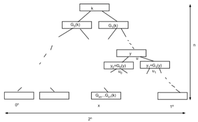
k G0(k) G1(k) y y0=G0(y) y1=G1(y) 0n 1n x Gxn...Gx1(k) u u0 u1 n 2n
Figure 9.2: The pseudorandom functionfk(x) outputs the label of thexthnode in a depthnbinary tree where the
root is labeled byk, and the childrenu0, u1of every nodeulabeledyare labeled byG0(y) andG1(y).
Theorem 9.16 ([GGM84])
Suppose that there exists a secure pseudorandom generator Gwith stretch `(n) = 2n. Then there exists a pseudorandom function family.
5In Chapter 18 we will see a stricter notion of expected probabilistic polynomial-time (see Definition 18.4). This
simulator satisfies this stricter notion as well.
6
p9.16 (174) 9.5. SOME APPLICATIONS
Proof:LetGbe a secure pseudorandom generator as in the theorems statement mapping length-n
strings to length-2nstrings. For everyx∈ {0,1}n, we denote byG0(x) the firstnbits ofG(x), and
by G1(x) the last nbits of G(x). For every k∈ {0,1}n we will define the functionfk(·) as follows:
fk(x) =Gkn(Gkn−1(· · ·(Gk1(x))· · ·) (10)
for every x∈ {0,1}n. Note that fk(x) can be computed by making ninvocations of G, and hence
clearly runs in polynomial time. Another way to view fk is given in Figure 9.2— think of a full
depth n binary tree whose root is labeled by k, and where we label the two children of a vertex labeled byy with the valuesG0(y) andG1(y) respectively. Then,fk(x) denotes the label of thexth
leaf of this tree. Of course, actually writing the tree down would take exponential time and space, but as is shown by (10), we can compute the label of each leaf in polynomial time by following the lengthnpath from the root to this leaf.
Why is this function family pseudorandom? We’ll show this by transforming aT-time algorithm
Athat distinguishes betweenfUnand a random function with biasinto a poly(n)T-time algorithm
B that distinguishes betweenU2n and G(Un) with bias /(nT).
Assume without loss of generality that Amakes exactly T queries to its oracle (we can ensure that by adding superfluous queries). Now, we can implement an oracle O tofUn in the following
way: the oracleOwill label vertices of the depthnfull binary tree as needed. Initially, only the root is labeled by a random stringk. Whenever, a query of A requires the oracle to label the children
u0, u1 of a vertexvlabeled byy, the oracle will invokeGonyto obtainy0=G0(y) andy1=G1(y)
and then label u0, u1 with y0, y1 respectively and delete the label y of u. Note that indeed, once
u0 and u1 are labeled, we have no further need for the label of u. Following the definition of fk,
the oracleOanswers a queryx with the label of thexthvertex. Note thatOinvokes the generator
G at most T n times. By adding superfluous invocations we can assume O invokes the generator exactlyT ntimes.
Now for everyi∈ {0, . . . , T n}define the oracleOias follows: the oracleOi follows the operation
ofO, but for the firstiinvocations ofG, instead of the labelsy0, y1 of the children of a node labeled
y by setting y0 = G0(y) and y1 = G1(y), the oracle Oi chooses both y0 and y1 independently at
random from{0,1}n. Note that O0 is the same as the oracle O tofUn, but OnT is an oracle to a
completely random function. Let pi = Pr[AOi(1n) = 1]. Then, as in the proof of Theorem 9.10,
we may assume pT n−p0 ≥ and deduce that Ei∈R[T n][pi−pi−1]≥ /(T n). Our algorithm B to
distinguish U2n from G(Un) will do as follows: on inputy∈ {0,1}2n, choose i∈R [T n] and execute
A with access to the oracle Oi−1, using random values for the first i−1 invocations of G. Then,
in the ith invocation use the value y instead of the result of invoking G. In all the rest of the invocations B runs G as usual, and at the end outputs what A outputs. One can verify that for every choice of i, if the input y is distributed as U2n then B’s output is distributed as AOi(1n),
while if it is distributed according toG(Un),B’s output is distributed as AOi−1(1n).
A pseudorandom function generator is a way to turn a random stringk∈ {0,1}ninto an implicit description of an exponentially larger “random looking” string, namely, the table of all values of the functionfk. This has proved a powerful primitive in cryptography. For example, while we discussed
encryption schemes for a single message, in practice we often want to encrypt many messages with the same key. Pseudorandom functions allow Alice and Bob to share an “exponentially large one-time pad”. That is, Alice and Bob can share a key k{0,1}n of a pseudorandom function, and whenever she wants to encrypt a message x ∈ {0,1}n for Bob, Alice will choose r ∈R {0,1}
n
, and send (r, fk(r)⊕x). Bob can findxsince he knows the keyk, but for an adversary that does not know
the key, it looks as if Alice sent two random strings (as long as she doesn’t choose the same stringr
to encrypt two different messages, but this can only happen with exponentially small probability). Pseudorandom functions are also used for message authentication codes. If Alice and Bob share
9.5. SOME APPLICATIONS p9.17 (175) a key k of a pseudorandom function, then when Alice sends a messagex to Bob, she can append the value fk(x) to this message. Bob can verify that the pair (x, y) he receives satisfiesy=fk(x).
An adversary Eve that controls the communication line between Alice and Bob cannot change the message x to x0 without being detected, since the probability that Eve can predict the value of
fk(x0) is negligible (after all, a random function is unpredictable). Furthermore, pseudorandom
function generators have also figured in a very interesting explanation of why current lower bound techniques have been unable to separate Pfrom NP; see Chapter 23.
9.5.2 Derandomization
The existence of pseudorandom generators implies subexponential deterministic algorithms for
BPP: this is usually referred to asderandomizationof BPP. That is, if L∈BPP then for every
> 0 there is a 2n-time deterministic algorithm A such that for every sampleable distribution of inputs {Xn} where Xn ∈ {0,1}n, Pr[A(Xn) = L(Xn)] > 0.99. (Note that the randomness is
only over the choice of the inputs— the algorithmA is deterministic.) The algorithm A works by simply reducing the randomness of the probabilistic algorithm for L to n using a pseudorandom generator, and then enumerating over all the possible inputs for the pseudorandom generator. We will see stronger derandomization results for BPPin Chapter 20.
9.5.3 Tossing coins over the phone and bit commitment
How can two parties A and B toss a fair random coin over the phone? (Many cryptographic protocols require this basic primitive.) If only one of them actually tosses a coin, there is nothing to prevent him from lying about the result. The following fix suggests itself: both players toss a coin and they take the XOR as the shared coin. Even if B does not trust A to use a fair coin, he knows that as long as his bit is random, the XOR is also random. Unfortunately, this idea also does not work because the player who reveals his bit first is at a disadvantage: the other player could just “adjust” his answer to get the desired final coin toss.
This problem is addressed by the following scheme, which assumes thatAandB are polynomial time turing machines that cannot invert one-way permutations. The protocol itself is called bit commitment. First,A chooses two stringsxAand rAof lengthnand sends a message (fn(xA), rA),
wherefn is a one-way permutation. This way,A commits the stringxA without revealing it. Now
B selects a random bit b and conveys it. Then A reveals xA and they agree to use the XOR of b
and (xArA) as their coin toss. Note thatB can verify thatxAis the same as in the first message
by applyingfn, thereforeA cannot change her mind after learningB’s bit. On the other hand, by
Theorem 9.11,B cannot predictxArA fromA’s first message, so this scheme is secure.
9.5.4 Secure multiparty computations
This concerns a vast generalization of the setting in Section 9.5.3. There are kparties and the ith party holds a stringxi ∈ {0,1}n. They wish to computef(x1, x2, . . . , xk) wheref:{0,1}nk → {0,1}
is a polynomial-time computable function known to all of them. (The setting in Section 9.5.3 is a subcase whereby each xi is a bit —randomly chosen as it happens—and f is XOR.) Clearly,
the parties can just exchange their inputs (suitably encrypted if need be so that unauthorized eavesdroppers learn nothing) and then each of them can compute f on his/her own. However, this leads to all of them knowing each other’s input, which may not be desirable in many situations. For instance, we may wish to compute statistics (such as the average) on the combination of several medical databases that are held by different hospitals. Strict privacy and nondisclosure laws may forbid hospitals from sharing information about individual patients. (The original example Yao gave in introducing the problem was of kpeople who wish to compute the average of their salaries without revealing their salaries to each other.)
p9.18 (176) 9.5. SOME APPLICATIONS We say that a multiparty protocol for computing f is secure if at the end no party learns anything new apart from the value of f(x1, x2, . . . , xk). The formal definition is inspired by the
definition of zero knowledge and says that whatever a party or a coalition of parties learn during the protocol can be simulated in an ideal setting where they only get to send their inputs to some trusted authority that computesf on these inputs and broadcasts the result. Amazingly, there are protocols to achieve this task securely for every number of parties and for every polynomial-time computablef— see the chapter notes.7
9.5.5 Lower bounds for machine learning
In machine learning the goal is to learn a succinct function f:{0,1}n → {0,1} from a sequence of type (x1, f(x1)),(x2, f(x2)), . . . , where the xi’s are randomly-chosen inputs. Clearly, this is
impossible in general since a random function has no succinct description. But suppose f has a succinct description, e.g. as a small circuit. Can we learnf in that case?
The existence of pseudorandom functions implies that even though a function may be polynomial-time computable, there is no way to learn it from examples in polynomial polynomial-time. In fact it is possible to extend this impossibility result to more restricted function families such as NC1 (see Kearns and Valiant [KV89]).
Chapter notes and history
We have chosen to model potential eavesdroppers, and hence also potential inverting algorithms for the one-way functions as probabilistic polynomial-time Turing machines. An equally justifiable choice is to model these aspolynomial-sized circuits or, equivalently, probabilistic polynomial-time Turing machines that can have some input-length dependent polynomial-sized constants “hard-wired” into them as advice. All the results of this chapter hold for this choice as well, and in fact some proofs and definitions become slightly simpler. We chose to use uniform Turing machines to avoid making this chapter dependant on Chapter 6.
Goldreich’s two volumes [Gol04] book is a good source for much of the material of this chapter (and more than that), while the undergraduate text [KL07] is a gentler introduction for the basics. For more coverage of recent topics, especially in applied cryptography, see Boneh and Shoup’s upcoming book [BS08]. For more on computational number theory, see the books of Shoup [Sho05] and Bach and Shallit [BS96].
Kahn’s book [Kah96] is an excellent source for the fascinating history of cryptography over the ages. Up until the mid 20th century, this history followed Edgar Alan Poe’s quote in the chapter’s start— every cipher designed and widely used was ultimately broken. Shannon [Sha49] was the first to rigorously study the security of encryptions. He showed the results presented in Section 9.1, giving the first formal definition of security and showing that to satisfy it it’s necessary and sufficient to have the key as large as the message. Shannon realized that computational difficulty is the way to bypass this bound, though he did not have a concrete approach how to do that. This is not surprising since the mathematical study of efficient computation (i.e., algorithm design and complexity theory) only really began in the 1960’s, and with this study came the understanding of the dichotomy between polynomial time and exponential time.
Around 1974, Diffie and Hellman and independently Merkle began to question the age-old no-tion that secure communicano-tion requires sharing a secret key in advance. This resulted in the groundbreaking paper of Diffie and Hellman [DH76] that put forward the notion ofpublic key cryp-tography. This paper also suggested the first implementation of this notion— what is known today
7
Returning to our medical database example, we see that the hospitals can indeed compute statistics on their combined databases without revealing any information to each other —at least any information that can be extracted feasibly. It is unclear if current privacy laws allow hospitals to perform such secure multiparty protocols using patient data— this an example of the law lagging behind scientific progress.
9.5. SOME APPLICATIONS p9.19 (177) as theDiffie-Hellman key exchange protocol, which also immediately yields a public key encryption scheme known today as El-Gamal encryption. But, to fully realize their agenda of both confidential and authenticated communication without sharing secret keys, Diffie and Hellman neededtrapdoor permutations which they conjectured to exist but did not have a concrete implementation for.8
The first construction for such trapdoor permutations was given by Rivest, Shamir, and Adleman [RSA78]. The resulting encryption and signature schemes were quite efficient and are still the most widely used such schemes today. Rivest et al conjectured that the security of their trapdoor per-mutation is equivalent to the factoring problem, though they were not able to prove it (and no proof has been found in the years since). Rabin [Rab79] later showed a trapdoor permutation that is in fact equivalent to the factoring problem.
Interestingly, similar developments also took place within the closed world of the intelligence community and in fact somewhat before the works of [DH76, RSA78], although this only came to light more than twenty years later [Ell99]. In 1970, James Ellis of the British intelligence agency GCHQ also realized that it might be possible to have secure encryption without sharing secret keys. No one in the agency had found a possible implementation for this idea until in 1973, Clifford Cocks suggested to use a trapdoor permutation that is a close variant of the RSA trapdoor permutation, and a few months later Malcolm Williamson discovered what we know today as the Diffie-Hellman key exchange. (Other concepts such as digital signatures, Rabin’s trapdoor permutations, and public key encryption from the codes/lattices seem not to have been anticipated in the intelligence community.) Perhaps it is not very surprising that these developments happened in GCHQ before their discovery in the open literature, since between Shannon’s work and the publication of [DH76], cryptography was hardly studied outside of the intelligence community.
Despite the well justified excitement they generated, the security achieved by the RSA and Diffie-Hellman schemes on their own was not fully satisfactory, and did not match the kind of security that Shannon showed the one-time pad can achieve in the sense of not revealing even partial information about the message. Goldwasser and Micali [GM82] showed how such strong security can be achieved, in a paper that was the basis and inspiration for many of the works that followed achieving strong notions of security for encryption and other tasks. Another milestone was reached by Goldwasser, Micali and Rivest [GMR84], who gave strong security definitions for digital signatures and showed how these can be realized under the assumption that integer factorization is hard.
Shamir [Sha81] first suggested that intractibility could be used to obtain a weak form of pseu-dorandomness known as block unpredictability. Blum and Micali [BM82] and then Yao [Yao82b] developed the stronger notion of pseudorandomness that is described in Section 9.2. The Goldreich-Levin theorem was proven in [GL89], though we presented an unpublished proof due to Rackoff . Theorem 9.8 and its very technical proof is by H ˙astad, Impagliazzo, Luby and Levin [HILL99] (the relevant conference publications are a decade older). The construction of pseudorandom functions in Section 9.5.1 is due to Goldreich, Goldwasser, and Micali [GGM84].
Zero knowledge proofs were invented by Goldwasser, Micali and Rackoff [GMR85]. Goldreich, Micali and Wigderson [GMW86] showed that if one-way functions exist then there is a computational zero knowledge proof system for every language in NP. The zero knowledge protocol for graph isomorphism of Example 9.14 is also from the same paper. Independently, Brassard, Chaum and Cr´epeau [BCC86] gave a perfect zero knowledge argument forNP(where the soundness condition is computational, and the zero knowledge condition is with respect to unbounded adversaries), under a specific hardness assumption.
Yao [Yao82a] suggested the first protocol for realizing securely any two party functionality, as
8Diffie and Hellman actually used the name “public key encryption” for the concept today known as trapdoor
permutations. Indeed, trapdoor permutations can be thought of as a variant of public key encryptions with a deterministic (i.e., not probabilistic) encryption function. But following the work [GM82], we know that the use of probabilistic encryption is both essential for strong security, and useful to get encryption without using trapdoor permutations (as is the case in the Diffie-Hellman / El-Gamal encryption scheme).
p9.20 (178) 9.5. SOME APPLICATIONS described in Section 9.5.4, but his protocol only worked for passive (also known as ”eavesdropping” or “honest but curious” adversaries). Goldreich, Micali and Wigderson [GMW87] extended this result for every number of parties and also showed how to use zero knowledge proofs to achieve security also againstactive attacks, a paradigm that has been used many times since.
Early cryptosystems were designed using the SUBSET SUM problem, but many of those were broken by the early 1980s. In the last few years, interest in such problems —and also the related problems of computing approximate solutions to the shortest and nearest lattice vector problems— has revived, thanks to a one-way function described in Ajtai [Ajt96], and a public-key cryptosystem described in Ajtai and Dwork [AD97] (and improved on since then by other researchers). These constructions are secure on most instances if and only if they are secure on worst-case instances. (The idea used is a variant of random self-reducibility.) See the book [MG02] and the survey [Reg06] for more on this topic. The hope is that such ideas could eventually be used to base cryptography on worst-case type conjectures such as P6=NPor NP∩coNP*BPP, but there are still some
significant obstacles to achieving this.
Much research has been devoted to exploring the exact notions of security that one needs for various cryptographic tasks. For instance, the notion of semantic security (see Section 9.2.2 and Exercise 9.9) may seem quite strong, but it turns out that for most applications it does not suffice and we need the stronger notion ofchosen ciphertext security [RS91,DDN91]. See the Boneh-Shoup book [BS08] for more on this topic. Zero knowledge proofs play a central role in achieving security in such settings.
Exercises
9.1. Prove that the one-time pad encryption is perfectly secret as per Definition 9.1.
9.2. Prove that if (E,D) is a scheme satisfying (1) with message-size m and key-sizen < m, then there exist two messages x, x0 ∈ {0,1}m such that EUn(x) is not the same distribution as
EUn(x
0).
Hint:Can all the distributions of the form EUn(x) have the same support?
9.3. Prove that in the one-time pad encryption, no eavesdropper can guess any bit of the plaintext with probability better than 1/2. That is, prove that for every function A, if (E,D) denotes
the one-time pad encryption then Pr k∈R{0,1} n x∈R{0,1} n [A(Ek(x)) = (i, b) s.t. xi =b]≤1/2.
Thus, the one-time pad satisfies in a strong way the condition (3) of computational security. 9.4. Exercise 9.2 and Lemma 9.2 show that for security against unbounded time adversaries (or efficient time ifP =NP) we need key as large as the message. But they actually make an implicit subtle assumption: that the encryption process is deterministic. In a probabilistic encryption scheme, the encryption function Emay be probabilistic: that is, given a message
x and a keyk, the value Ek(x) is not fixed but is distributed according to some distribution
Yx,k. Of course, because the decryption function is only given the keykand not the internal
randomness used byE, we modify the requirement (1) to requireDk(y) =xforevery y in the
support of Ek(x). Prove that even a probabilistic encryption scheme cannot have key that’s
significantly shorter than the message. That is, show that for every probabilistic encryption scheme (D,E) using n-length keys and n+ 10-length messages, there exist two messages
x0, x1 ∈ {0,1}n+10 and functionA such that
Pr
b∈R{0,1} k∈R{0,1}
n