CHARACTERIZATION OF DIESEL SPRAY IMAGES USING A SHAPE PROCESSING METHODOLOGY

CHARACTERIZATION OF DIESEL SPRAY IMAGES USING A SHAPE

PROCESSING METHODOLOGY

C

ECILE

P

ETIT1,2

, W

OLFGANG

R

ECKERS2

, J

EAN

-M

ARIE

B

ECKER1,3 AND

M

ICHEL

J

OURLIN1

1_{TSI Laboratory (Traitement du Signal et Instrumentation, UMR 5516 CNRS, Saint-Etienne, France);} 2_Delphi

(Technical Center Luxembourg); 3_{CPE Lyon (Ecole Supérieure de Chimie, Physique, Electronique, Lyon, France)}

e-mail: [email protected], [email protected], [email protected], [email protected] (Accepted April 25, 2005)

ABSTRACT

In Diesel engines, a key element in achieving a clean and efficient combustion process is a proper fuel-air mixing, which is a consequence of the fuel spray development and fuel-air interaction inside the engine combustion chamber. The spray structure and behavior are classically described by the length (penetration) and width (angle) of the spray plume but these parameters do not give any clue on the geometrical injection center and on the spray symmetry. The purpose of this paper is to find out original tools to characterize the Diesel spray: the virtual spray origin is the geometrical injection center, which may (or may not) coincide with the injector axis. Another interesting point is the description of the Diesel spray in terms of symmetry: the spray plume internal and external symmetry characterize the spray and the injector performance. Our approach is first to find out the virtual spray origin: after the image segmentation, the spray is coded with the Freeman code and with an original shape coding from which the moments are derived. The symmetry axes are then computed and the spray plumes are discarded (or not) for the virtual spray origin computation, which is derived from a Voronoi diagram. The last step is the internal and external spray plume symmetry characterization thanks to correlation and mathematical distances.

Keywords: Diesel sprays, Freeman coding, image processing, moments, symmetry, Voronoi diagram.

INTRODUCTION

The key element of combustion engines is their combustion chamber. In a Diesel combustion chamber, the injector is usually placed at the top of the chamber, delivering fuel inside it. When the piston moves up, temperature and pressure raise, the spray evaporates and the swirl transports the fuel droplets and the vapor.

Fig. 1. A Diesel combustion chamber.

Present day investigations about Diesel sprays all aimed at the reducing of pollutant emissions, without harming efficiency. Ideally, the spray should not hit the chamber walls, avoiding thus the creation of pollutant emissions, but should penetrate enough inside the

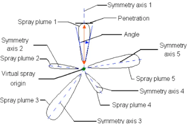
chamber for providing the right mixing between air and fuel. Classically, the individual spray plumes penetration and angle (as defined on Fig. 2) are computed to understand the spray evolution inside the combustion chamber in terms of length and width. Empirical relations between these parameters have been established in Lefebvre (1989).

The automated calculation of these parameters relies on an accurate determination of the virtual spray origin (VSO). Moreover, the comparison between the respective positions of the VSO and the “true” injector axis should provide an evaluation of the Diesel spray, as in the perfect case the injector axis and the VSO are coincident.

Other spray parameters may be defined in order to characterize individual spray plumes or to compare spray plumes: internal and external symmetry tools provide information about the fuel flow and the injector performance. Indeed, when the internal and external symmetry of a single spray plume is perfect, it indicates not only a symmetric flow but also an efficient injector design regarding those parameters. The comparison spray plume to spray plume quantifies the flow similarity coming out of the injector, its design symmetry and performance.

This paper presents a method to compute the virtual spray origin of a Diesel spray which is the injection center, then different tools to characterize the spray plume internal and external symmetry are presented. The virtual spray origin calculation was first done manually in Le Visage et al., (1997) but this method was subjective and not accurate. Then, an algorithm based on a sliding mask positioning was developed by Lliasova et al., (1998), but when the spray plumes positions change, the virtual spray origin would be shifted (hence would not correspond to the real origin). Concerning the spray plumes symmetry study, the authors have not found any reference on the topic in the literature.

THE STATE OF THE ART IN DIESEL

SPRAYS IMAGING

Different optical techniques permit to obtain quantitative or qualitative information about fuel liquid and vapor.

Several visualization techniques exist, as backward or forward scattering, holography, tomography, endoscopic measurements, Fraunhofer diffraction. The articles by Chigier (1991) and Hiroyasu et al., (2002) review in depth existing techniques for liquid and/or vapor phases visualization, providing (or not) the concentration information.

Backward or forward methods are mainly used to assess in a qualitative way the spray liquid phase. Its principle relies on the Mie theory explained in Van de Hulst (1957) based on the scattering of light by spherical droplets. The qualitative observation of the vapor phase can be done thanks to the Schlieren

technique, which permits the observation of the refractive index gradient. The Background Oriented Schlieren (BOS) is described in Richard et al., (2001).

Quantitative liquid and vapor phases visualizations are possible using Laser Induced Exciplex Fluore-scence (LIEF) presented in Kim et al., (2001). This method, using a dopant, provides simultaneously the concentration of the liquid and of the vapor phases, using the excitation of these phases by an excimer laser causing the fluorescence of the liquid and vapor at different wavelengths.

Another method referred to as the Laser Absorption Scattering technique (LAS) described in Zhang et al., (2003), permits the observation of the droplets and the vapor distributions thanks to the measurement of the droplets optical thickness (visible light) and to the joint vapor and droplets optical thickness (ultraviolet light). This dual wavelength method needs 1-3 dimethyl -naphthalene as test fuel which strongly absorbs ultraviolet light and is nearly transparent to visible light.

METHODS

IMAGE ACQUISITION DEVICE.

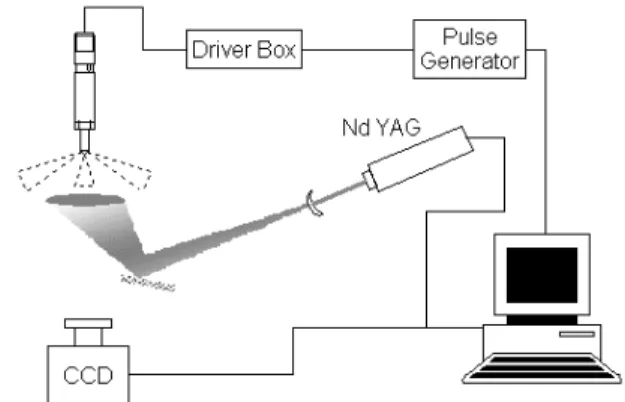
The device used is schematized on Fig. 3. It is based on the backward scattering of light by the fuel droplets presented in Chigier (1991), giving qualitative information about the liquid phase.

Fig. 3. The optical device used for image acquisition. The pulse generator delivers a reference signal to the injector driver box and the imaging system, which then triggers the light source and the CCD camera. Images are taken during the light flashes.

IMAGE PROCESSING STEPS.

be subtracted from the raw image, and then a reference image (taken with a uniform white screen) is used to decrease the effect of non-homogeneous illumination. Additional filtering may be necessary; median filter can as well be used carefully because the contrast is sensitive to filtering.

The next step is segmentation. The spray object is determined using Entropy Maximization method defined in Pun (1981). The principle of this segmentation is the maximization of the image entropy (in the Shannon sense).

Then the inside boundary of the objects is calculated with a sliding pattern, and afterwards coded with a Freeman 4 – code presented in Freeman (1974).

(a)

(b)

Fig. 4. (a) A shape contour coding with the Freeman 4 - code and the edges indexing. (b) The vertices indexing.

VIRTUAL SPRAY ORIGIN (VSO)

CALCULATION

VSO is based on the spray plumes symmetry axes computation. Indeed, all the axes of regularly shaped sprays (elongated spray plumes), should approximately meet at the VSO vicinity (see Fig. 2):

A raw virtual spray origin (RVSO) is first determined as the barycenter of the symmetry axes intersections; then the accurate virtual spray origin (AVSO) is found using the Voronoi diagram.

In order to compute the RVSO, the spray plumes symmetry axes have to be determined.

The symmetry axis of a regular 2D object should be the primary principal axis. By definition, the secondary principal axis is perpendicular to the first one intersecting it into the shape’s center. These two principal axes define the dispersion of the shape in two dimensions. They can be simultaneously obtained

by minimization of inertia J about an axis ∆ (dist refers to distance). Freeman (1974) described a computation of the shape’s moments of inertia of order (p, q) using Freeman 4 – code. The approach taken here is more general but it is described in detail.

(a)

(b)

(c)

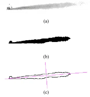
Fig. 5. (a) Input spray plume and its principal axes. (b) Segmented image. (c) Freeman 4 - code of the spray plume and its principal axes.

Inertia J is calculated with this formula:

( )

(

)

[

]

∫∫

∈

∆ =

object P

dxdy axis

y x P dist

J , , 2 . (1)

Using the parametric definition of a line (θ,p), Eq. 1 becomes:

(

)

∫∫

∈

−

+

=

S y x

dxdy

p

y

x

J

) , (

2

sin

cos

θ

θ

. (2)

The issue is to find θ and p such that J is minimal, or more generally, extremal.

Let us consider a closed contour coded with the Freeman 4 - code. This closed contour has an even number of edges (2n), its vertices are S0, S1, …, S2n-1

(with S0 = S2n). Concerning the initialization, S0(x0,

y0) is chosen as one of the vertices (there may be

more than one such point) which is reached on its north side and left on its east side. The vertices are indexed according to an anticlockwise direction. An even index vertex S2k has (xk, yk) as its coordinates,

an odd index vertex S2k+1 has (xk+1, yk) as its

coordinates (see Figs. 4a,b). In this way the sequence of vertices is:

(

) (

) (

)

(

)

By definition, the shape moment of order (p,q) is: ( )

∫∫

∈

=

object y x q p

pq

x

y

dxdy

I

;

, (4)

which can be shown to be (using the preceding coding scheme):

(

)(

)

(

)

(

)(

)

∑

(

)

∑

− = + + + + + − = + + + +

−

+

+

=

−

+

+

=

1 0 1 1 1 1 1 1 0 1 1 1 1

1

1

1

1

1

1

n k q k q k p k n k q k p k p k pq

y

y

x

q

p

y

x

x

q

p

I

. (5)

We emphasize the fact that the shape we consider is an object with a “continuous” meaning, not just a discrete set of pixels: it is the subset of the place delimited by the Freeman – coded boundary.

Using these notations, the expansion of Eq. 2 gives (with

X

=

(

x

₁

,

x

₂

,

x

₃

) (

=

cos

θ

,

sin

θ

,

−

p

)

:

[

]

          −             − = = p p AX X J

I

I

I

I

I

I

I

I

I

T θ θ θ θ sin cos sin cos 00 01 10 01 02 11 10 11

20 . (6)

The problem is to minimize XT_{AX under}

1

2 2 2

1

+

x

=

x

constraint. Let us consider the following matrixes

A

~

=

det(

A

).

A

−1 (adjoint matrix of A) and matrix K (which plays a technical role):

2 11 02 20 01 20 10 11 10 02 01 11 2 01 00 20 00 11 01 10 2 01 00 02

~

I

I

I

f

I

I

I

I

e

I

I

I

I

d

I

I

I

c

I

I

I

I

b

I

I

I

a

f

e

d

e

c

b

d

b

a

A

−

=

−

=

−

=

−

=

−

=

−

=





















=

, (7)           = 0 0 0 0 1 0 0 0 1

K . (8)

The problem is equivalent to minimizing XTAX under the constraint KX =1. Using a Lagrange multiplier described in Strang (1986), we can replace this minimization by:

KX A X KX A X KX AX ad = ⇔ = ⇔ = −

µ

λ

λ

1

1 _{, (9)}

for a certain µ.

In this way X appears as an eigenvector associated with eigenvalue µ of the following:

          = = 0 0 0 e d c b b a K A

B ad _{. (10)}

Let us attribute the following names:

      = c b b a

M , (11)

[

d e

]

VT _{= . (12)}

Let Xk (k = 12) be an eigenvector of M associated to (non zero !) eigenvalue λk. It is easy to verify that

      k T k k k X V X λ λ2

(which belongs to R3_{) is an eigenvector}

of B possessing the desired structure

          − p

θ

θ

sin cos

if

X

_k

is taken such that 2 ₌1

k k X

λ

which is always

possible.

We do not give here the computational details of how to obtain Xk and λk because they are quite standard. From here, we obtain: θ = polar angle of Xk and p = –λkVTXk.

SPRAY PLUMES DISCARDING

The principal axes calculation works well on regular shaped spray plumes.

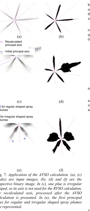
Concerning irregular shaped spray plumes, Fig. 7e clearly shows a typical case where some irregular shaped spray plumes must be discarded for the RVSO calculation in order to be reexamined later on, once the AVSO has been determined.

Once the first and second inertia axis are determined, their inertia J’ and J” can be readily obtained using Eq. 6.

Once this discarding process is done, the non discarded main axes intersect at different points; their barycenter is the RVSO.

ACCURACY ENHANCEMENT WITH THE

VORONOI DIAGRAM

By definition, the AVSO should be the nearest point to the spray plumes.

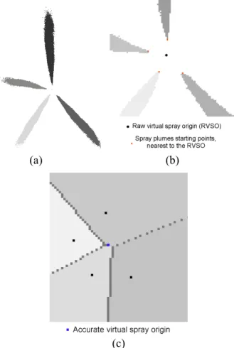
In the Voronoi diagram, each Voronoi vertex is the nearest point to three sites. Thus the Voronoi vertex barycenter is the nearest point to the set of sites. In our case, this principle may be applied; the sites would be the spray plumes starting points (calculated thanks to the RVSO), the AVSO is then the barycenter of the Voronoi diagram vertices. An example is given in Fig. 6, with labeled spray plumes and cells.

(a) (b)

(c)

Fig. 6. (a) Labeled spray plumes after sorting. (b) Zoom on image (a). (c) Labeled Voronoi diagram of the spray plumes starting points.

RESULTS AND DISCUSSION

EXAMPLES OF THE INERTIA AXES AND

OF THE AVSO CALCULATIONS

In Fig. 5, the first image is an input single spray plume. The binary image is computed, and then the Freeman 4 - code defined in Freeman (1974) of the shape is derived and the first and second principal axes are determined.

Examples of the AVSO calculation may be observed in Fig. 7.

AXES RECALCULATION FOR

DISCARDED SPRAY PLUMES

As explained before, some spray plumes may have been discarded for the RVSO calculation. It may be interesting to calculate the first principal axis of these discarded spray plumes, knowing that this axis should minimize inertia J (Eq. 6), with the constraint that AVSO should belong to this axis.

If (x0,y0) are the AVSO coordinates, the parametric

representation (θ, p) of the corresponding axis is determined by:

0 sin

cos

0

0

0 + − =

=

p y

x

d dJ

θ

θ

θ

. (13)

It can be shown that a solution of Eq. 13 is:













−

=

B

A

C

Arc

tan

2

1

θ

, (14)

θ

θ

sin

cos

₀

0

y

x

p

=

+

, (15)

with:

(

11 0 0 00 0 10 0 01

)

01 0 00 2 0 02

10 0 00 2 0 20

2

2

2

I

x

I

y

I

x

y

I

C

I

y

I

y

I

B

I

x

I

x

I

A

−

−

+

=

−

+

=

−

+

=

. (16)

(a) (b)

(c) (d)

(e) (f)

Fig. 7. Application of the AVSO calculation. (a), (c) and(e) are input images, (b), (d) and (f) are the respective binary image. In (c), one plue is irregular shaped, so its axis is not used for the RVSO calculation, the recalculated axis, processed after the AVSO calculation is presented. In (e), the first principal axes for regular and irregular shaped spray plumes are represented.

INTERNAL SYMMETRY OF A SINGLE

SPRAY PLUME

The spray plumes principal axes have been calculated beforehand. Now, it would be interesting to know the single spray plumes symmetry by comparing their interior and exterior. Note that the tools presented in this part could be used to compare spray plumes

between themselves which could indicate the similarity between two spray plumes. Furthermore, the spray uniformity could be derived calculating a single correlation (or distance) for the whole spray.

The spray plume interior can be analyzed using one of the distances (17), (18), (19). h(u, v) (resp. q(u, v)) is the grey level of the (u, v) pixel in the first (resp. second) image.

( ) ( )

∑

−

=

v u

v

u

q

v

u

h

n

d

,

1

,

,

1

, (17)

( ) ( )

(

)

∑

−

= v u

v u q v u h n d

,

2

2 , ,

1

, (18)

( ) ( )

(

h u v qu v

)

d

v u

, ,

sup

,

− =

∞ , (19)

n refers to the number of couples

(

h

( ) ( )

u,v ,q u,v

)

. A symmetrized spray plume with respect to its axis is calculated; then the input spray and the symmetrized spray plume are compared pixel to pixel as shown on Fig. 8.

(a)

(b)

Fig. 8. (a) Input spray plume. (b) Symmetrized spray plume with respect to the axis.

The correlation coefficient measures the degree of similarity between two sets of data. In our application, the first image (x) refers to as the input spray plume and the second image (y) refers to as the perfectly symmetric spray plume with respect to the axis (see Fig. 8). Between these two images, one half part is

Recalculated principal axis

Initial principal axis

R for regular shaped spray plumes

completely equal (as the mirror spray plume has been created, see Fig. 8b), so the correlation will only depend on the two different half parts, thus it amounts to the computation of the correlation coefficient between the two initial half parts of the input spray plume.

Let us define the ascending order of the first image grey levels’ x1 < ... <xi< ... < xk and the ascending order of the second image grey levels’ y1 < ... <yj< ... < yl.

ni represents the number of pixels of grey level xi

in the first image.

nj represents the number of pixels of grey level yj

in the second image.

ni ,j is the number of pixels characterizing the grey

levels (xi, yj): let us assume we are computing ni ,j and

that the pixel under study coordinates are (u, v). If this pixel has xi as grey level in the first image and

has yj as grey level in the second image, one is added

to ni ,j, and so on ….

With this scheme, the correlation coefficient r is computed:

( )













−













₋

⋅

−

=

=

∑

∑

∑

= =

=

2

1 2 2

1 2

,

1 ,

2 2

,

cov

y

N

y

n

x

N

x

n

y

x

N

y

x

n

y

x

r

l j

j j k

i i i

l k

j

i ij i j y x

σ

σ

, (20)

with:

∑∑

∑

∑

∑

∑

= =

= =

= =

=

=

=

=

=

k i

l j

j i

l i i j j

k j i j i

l j j j k

i i i

n

N

n

n

n

n

y

n

N

y

x

n

N

x

1 1

,

1 ,

1 ,

1 1

1

1

. (21)

In Diesel spray applications, the correlation coefficient represents the similarity between the two half parts of the input spray plume. Quantitative measurements (see the state of the art in Diesel sprays imaging) are said to provide the concentration of the liquid and/or the vapor phases. Using this tool on quantitative images would indicate the dispersion of the studied phase with respect to the axis, in terms

of concentration. The calculation of the correlation coefficient between the different single spray plumes would measure the studied phase similarity and its calculation for the whole spray would indicate the flow uniformity, providing an assessment about the injector design.

EXTERIOR SYMMETRY OF A SINGLE

SPRAY PLUME.

The interior of the spray has been characterized, it would be interesting to get the exterior of the spray symmetry. In fact, other tools can be used to determine the object boundary similarity in terms of distance, orientation and shape.

The first principal (or the recalculated) axis of the object is known, as presented in Fig. 9. The idea is to calculate the distances between the two sub boundaries of the object, with respect to the symmetry axis.

(a)

(b)

Fig. 9. (a) The spray plume boundary and its symmetry axis. (b) The perfect symmetric spray plume boundary.

In order to get the two sub boundaries of the spray plume with respect to the symmetry axis, the mirror image spray around the axis is calculated (see Fig. 9). One spray plume half part is arbitrarily chosen and is mirrored. Choosing this half part or the other one does not change anything for the tools computation.

Fig. 10. The two sub chains f and g comparison. f refers to the lower part of Fig. 9a, g refers to the lower part of Fig. 9b.

Let us refer to the two sub boundaries by f and g and to their area under graph by AG( f ),AG( g ). Getting the differences between f and g may be done by comparing their area under graph. The absolute, the Euclidean, the infinite and the Hausdorff distances can be used to compare them. If f (resp. g) has only one value for a given i, then

( )

( )

f i f

( )

i

AG = (resp. AG

( )

g

( )

i = g

( )

i ).

(

)

_∑

( )

( )

( )

( )

=

− Μ

= b

a i

i g AG i f AG g

f

d₁ , 1 , (22)

(

)

( )

( )

( )

( )

(

)

2

1 2 2

1

,

   



 ₋

Μ

=

∑

= b a i

i g AG i

f AG

g f d

, (23)

(

)

[ ]AG

( )

f

( )

i AG

( )

g

( )

i

g f d

b a i

− =

∈ ∞

,

sup

, . (24)

M refers to the number of couples (AG( f (i)), AG( g (i))).

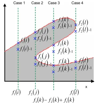
Let us explain the calculation of (AG( f (i)). It might happen that for a given i, f(i) (resp. g(i)) have more than one value which can be written (see Fig. 11):

( )

i

f

( )

i

f

( )

i

f

₁

<

₂

<

...

<

_n . (25) To calculate the area under graph, all intersection points

f

₁

( ) ( )

i

...

f

_n

i

have to be scanned. Once the first point belonging to the plume has been found, each intersection

f

_h

( )

i

has to be sorted as belonging (or not) to the object. Then, at each change (outside of object – inside of object, or the contrary) after the first point belonging to the object, a corresponding sign is affected (positive for outside of object – inside of object, or negative for the contrary).

( )

j f₂ -1

( )

j

f

1

x y

( )

l

f

₁

( )

k f₃ -1

( )

l f2 -1

( )

l f₂

( )

i f₁ -1

( )

j

f

₁ -1

( )

k f₃

Case 1 Case 2 Case 3 Case 4

( )

l

f

₁ -1

( )

k

f

₂ -1

( )

k

f

₁ -1

( )

j

f

₂

( )

i f₁

( )

k

f

₁

( )

k f₂

( )

i

f₁ f₂

( )

j

( )

k f

( )

k f

( )

k f₃ − ₂ + ₁

( )

l f₁

Fig. 11. External symmetry parameters: calculation of distances between the boundaries.

The scanning of the intersections has to be done from the top, a simple test is implemented: as

f

_n

( )

i

is the first intersection encountered by the top,

( )

( )

[

f

_n

i

,

f

_n−1

i

]

must represent the object if the pixel

( )

i

−

1

f

_n is within the object, otherwise this segment is empty. Afterwards,

[

f

_n−1

( )

i

,

f

_n−2

( )

i

]

has to be classified as belonging (or not) to the object thanks to testing if

f

_n−1

( )

i

−

1

is within the object and so on… The formula to calculate the area under graph may be derived, a positive sign represents the object, a negative one an empty segment, only changing object state are taken into account. Fig. 11 illustrates the calculation of AG( f (i)) for different values of i.

Note that the Hausdorff distance corresponds to the maximal distance between two objects, regarding all directions. It is calculated with dilations. One sub boundary is selected and dilated until the other object is completely included in it. The number of dilations α is recorded. Then, coming back to the initial figure, the second sub boundary is selected and dilated until the first one is completely included. The number of dilations β is recorded. The Hausdorff distance is calculated using Eq. 26.

(

f g

)

(

)

mask size

d_H , =max

α

,

β

⋅ . (26)

and B coded with the Freeman 8 - code. If the comparison is made between the initial and the perfect symmetric object, the correlation between the two equal parts will be one; so the correlation only depends on the two different parts.

Thus the shape boundaries are coded with the Freeman 8 - code and the correlation is calculated, as defined in Freeman (1974):

( )

_∑

(

)

= +

− =

Φ

≤ =

=

n i

j i i ab

m n

b a n

j

m n b b b B

a a a A

1 2 1

2 1

4 cos

1 ...

...

π

. (27)

It is an average pair-wise alignment between A and B giving an indication of the shape congruence for different shifts of B relative to A.

Note that ai and bj are between 0 and 7, as given

in Fig. 12.

Fig. 12. Links ai and bj values: the Freeman 8 - code. As we want to know the similarity between the two sub chains, the correlation function is maximized:

[ ]_n

(

ab

( )

j

)

j

ab = Φ

Φ

∈1,

max . (28)

Note that the complete initial spray plume and the perfect symmetric spray plume are used because we are sure that the maximization will happen if the two equal sub parts correspond (see Fig. 13).

INTERNAL AND EXTERNAL SYMMETRY

OF A SPRAY PLUME: SOME

APPLICATION EXAMPLES

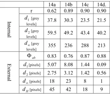
Single spray plumes of Fig. 14 were analyzed. The results are presented in Table 1.

The use of all developed tools should make it possible to select a good spray plume in terms of internal and external symmetry. Fig. 14 presents some more or less symmetric, elongated plumes. Plume 14a shows an elongated shape with a fine (but not perfect) external symmetry. The grey levels distribution on both sides of the symmetry axis is not homogeneous. Plume 14 b presents a compact shape with an asymmetric boundary. Its grey level distribution on both sides of the symmetry axis is symmetric. Plume 14c shows an

elongated shape with fine external and internal symmetries, those could be better, as presented by plume 14d which is the best in terms of shape, internal and external symmetry.

Fig. 13. Comparison between the input and the perfect symmetric spray plume when the correlation is maximum.

14a 14b 14c 14d.

r 0.62 0.89 0.90 0.90

1

d [grey

levels] 37.8 30.3 23.5 21.5

2

d [grey

levels] 59.5 49.2 43.4 40.2

Internal

∞

d [grey

levels] 355 236 288 213

ab

Φ

0.83 0.76 0.87 0.88

1

d [pixels] 5.07 8.08 1.44 0.09

2

d [pixels] 2.75 3.12 1.42 0.56 ∞

d [pixels] 18 23 8 1

External

H

d [pixels] 45 42 18 9 Table 1. Internal and external symmetry of spray plumes 14a to 14d.

The calculated parameters for correlation r (internal) and Φ (external) vary between 0 (completely asymmetric) to 1 (perfectly symmetric). For the internal symmetry, the absolute distance d1, defined

by Eq. 17, is an average grey level difference between symmetric pixels. The Euclidian distance d2, presented in Eq. 18, represents a similar information, but an emphasis is put on the grey levels difference, thanks to the square. The infinite distance d∞, defined in Eq.

19, is the maximum difference of grey levels between two symmetric pixels. Concerning the external symmetry, the absolute distance d1 (see Eq. 22) is an

Coincidence between the two half parts of the object

Perfect symmetric spray plume: the second half part

averaged distance between the two boundaries in the perpendicular direction. Like the internal symmetry, the Euclidian distance d2 (Eq. 23) puts an emphasis

on the boundaries difference. The infinite distance d∞

(Eq. 24), is the maximum distance between the two boundaries in the perpendicular direction. The Hausdorff distance (Eq. 26) is the maximum distance between the two boundaries in all directions.

(a)

(b) (c) (d)

Fig. 14. Analyzed spray plumes in terms of internal and external symmetry.

Values of Table 1 provide criteria for plume selection. Fig. 14a shows (in line with the observation above) a low internal symmetry correlation r. Fig. 14b has been rejected for spray origin calculation due to its shape (ratio J’’/J’), additionally the external symmetry coefficient Φ is low as observed above. Fig. 14c is described by the parameter r, Φ as internally and externally symmetric and by d1, d2 as

not externally symmetric which correspond to its description. Finally all parameters show that Fig. 14d is internally and externally symmetric, as expected.

The parameters shown in Table 1 clearly describe relevant spray characteristics and enable automated injector evaluation using image processing and data reduction. Improvements on the dynamic range of the parameters are under investigation in order to enhance the differentiation between the studied plumes.

This paper has presented an original methodology for automatically computing diesel spray characteristics by taking into account the specific geometry of the involved shapes. Different tools for the individual spray plume characterization in terms of interior and

exterior symmetry were presented. These latest tools could also be used for spray plumes comparison.

The interest of this method is to automatically compute an accurate virtual spray origin as well as symmetry tools which are easily understandable by the users.

The next step in our investigation will be to efficiently characterize the whole spray in terms of spray plumes penetration, angle, similarity with original tools. Then spray vapor phase studies will complete the diesel spray characterization.

This method has the potentiality to be extended to other kinds of spray (water, perfumes…).

REFERENCES

Chigier N (1991). Optical imaging of sprays. Prog Energy Combustion Science 17:211-62.

Freeman H (1974). Computer processing of line - drawing images. Computing Surveys 1:57-97.

Hiroyasu H, Miao H (2002). Optical techniques for diesel spray and combustion. Thiesel conference on thermo and fluid dynamic processes in diesel engines, Valencia, Spain.

Kim JU, Hong B (2001). Quantitative vapour-liquid visualization using laser-induced exciplex fluorescence. J Optics A: Pure and Applied Optics 3:338-45.

Le Visage D, Berdah D, Trémoulière G (1997). Visualisation ultra-rapide et traitement d'images appliqués à la caractérisation de jets d'injecteur diesel. Visualisation et traitement d'images en mécanique des fluides. Colloque national VISU, Saint Louis France.

Lefebvre AH (1989). Atomization and sprays. Bristol: Taylor and Francis.

Lliasova NYu, Ustinov AV, Bystrov NV, Medinskaya LN (1998). Evaluating the geometrical parameters of images of atomization jet cross-section in diagnostics of diesel injectors. Proceedings of the SPIE, the International Society for Optical Engineering, 3348:308-15.

Pun T (1981). Entropic thresholding: a new approach. Computer Vision - Graphics and Image Processing 16: 210-39.

Richard H, Raffel M (2001). Principle and applications of the background oriented Schlieren (BOS) method. Measurement Science Technology 12:1576-85. Strang G (1986). Introduction to Applied Mathematics.

Wellesley: Wellesley-Cambridge Press.

Van de Hulst HC (1957). Light scattering by small particles. New-York: John Wiley and Sons.