CONTENT BASED VIDEO RETRIEVAL BASED ON HDWT AND SPARSE REPRESENTATION

CONTENT BASED VIDEO RETRIEVAL BASED ON HDWT AND

SPARSE REPRESENTATION

S

M

H

F

Department of Electronics and Communications Engineering, University of Birjand, Birjand, Iran e-mails: [email protected]; [email protected];

(Received May 30, 2015: revised November 24, 2015; revised February 13, 2016; accepted March 29, 2016)

ABSTRACT

Video retrieval has recently attracted a lot of research attention due to the exponential growth of video datasets and the internet. Content based video retrieval (CBVR) systems are very useful for a wide range of applications with several type of data such as visual, audio and metadata. In this paper, we are only using the visual information from the video. Shot boundary detection, key frame extraction, and video retrieval are three important parts of CBVR systems. In this paper, we have modified and proposed new methods for the three important parts of our CBVR system. Meanwhile, the local and global color, texture, and motion features of the video are extracted as features of key frames. To evaluate the applicability of the proposed technique against various methods, the P(1) metric and the CC_WEB_VIDEO dataset are used. The experimental results show that the proposed method provides better performance and less processing time compared to the other methods.

Keywords: content based video retrieval (CBVR), Hadamard matrix and discrete wavelet transform (HDWT), key frame extraction, shot boundary detection, sparse representation.

INTRODUCTION

Video data contains several types of information such as images, sounds, motions, and metadata. These characteristics have caused research in processing videos to become quite difficult and time consuming. Video retrieval is used in numerous multimedia sys-tems, processing and applications, and also assisting people in finding the videos, images and sounds related to the user’s interest. In early video retrieval systems, videos were manually annotated using text descriptors. However, these systems have several shortcomings. For example, the concept of a video is more than a series of words, since manual indexing is a costly and difficult process. Due to increasing the number of video datasets and as well as the mentioned shortcomings, text based video retrieval is known to be an inefficient method, while the demand for CBVR increases. The content based techniques use vision features for the interpretation of the videos (Lew et al., 2006).

CBVR systems are useful for a wide range of applications such as seeking an object in a video, digital museums, video surveillance, video tracing, and management of video datasets, as well as remote controlling, and education.

Video involves visual information, audio infor-mation and metadata (Chung et al., 2007). Visual information contains numerous frames and objects, and their feature vectors are extracted by content based methods. Audio information can be obtained by speech recognition methods, and video indexing by using extracted texts. Metadata contains the title, date, sum-mary, producer, actors, file size, and so on. These types data are often used for video retrieval. CBVR systems contain three important parts, 1) shot boundary detec-tion, 2) key frame extracdetec-tion, and 3) video retrieval. There is plenty of research in all of these areas, and the novel methods are well-motivated in recent years (Weiming et al., 2011). In the following, we review the processes and recent developments in each area.

methods have been proposed to detect abrupt and gradual transitions (Smeaton et al., 2010). The shot boundary detection methods usually have three main steps. In the first step, visual features of each frame are extracted by using special methods. These features include histogram, edge, color, texture, motion features, and scale invariant feature transform (SIFT) (Porter, 2004; Chang et al., 2008). Then, the similarity is measured between these extracted features. Many similarity measurements have been proposed by resear-chers, such as the Euclidean distance, the cosine dis-similarity, the earth mover’s distance, and the histo-gram intersection (Hoi et al., 2006; Camara et al., 2007). The similarity is measured between consecutive frames or between a limited number of frames located in a window (Hoi et al., 2006). Finally, the shot boundaries between dissimilar frames are detected. The shot boundary detection methods can be classi-fied into two approaches: 1) statistical learning-based, such as support vector machine (SVM) (Matsumoto

et al., 2006), Adaboost, k nearest neighbor (kNN), Hidden Markov Models (HMM), and clustering algo-rithms such as K-means and fuzzy K-means (Damnja-novic et al., 2007) 2) threshold-based approaches which detect the boundaries by comparing the measured pair-wis a predefined threshold (Cernekova

et al., 2006; Weiming e similarities between frames with et al., 2011).

After shot boundary detection, the key frame extraction is the second important part of the video retrieval systems. The frames within the shot contain great redundancies and similar contents. Therefore, the key frames should be extracted to summarize the video, and succinctly represent the shot (Mukherjee

et al., 2007). In the last decade, several features for key frame extraction have been proposed such as: colors (e.g. histogram), textures (e.g. discrete wavelet transform, discrete cosine coefficient), shapes, motions (e.g. motion vectors, image variations), and optical flow (Narasimha et al., 2003; Guironnet et al. 2007; Wang et al., 2007). Truong and Venkatesh have classified the key frames extraction methods into six categories (2007): clustering based (Yu et al., 2004), sequential comparison-based (Zhang et al., 2003), global comparison-based (Liu et al., 2004), reference frame-based (Ferman and Tekalp, 2003), object/event-based (Song and Fan, 2006) and curve simplification-based (Calic and Izquierdo, 2002).

Finally, the video retrieval part is applied to show the retrieval results. According to Weiming et al. (2011) the six types of query has been proposed: 1) query by example, 2) query by sketch, 3) query by object, 4) query by keywords, 5) query by natural language, and

6) combined based query. In this paper, the query by example has been used. This query extracts low-level features from given example videos or images, and similar videos or key frames are found by measuring the feature similarities. The static feature of key frames are suitable for query by example, as the key frames extracted from the example videos or exemplar images can be matched with the stored key frames (Weiming

et al., 2011). The stored key frames complements video retrieval (Xiong et al., 2006), by making browsing of the retrieved videos faster, especially when the total size of the retrieved videos is large. The user can browse through the abstract representations to locate the desired videos. A detailed review on video browsing interfaces, and applications can be found in (Schoeffmann et al., 2010). There are two basic strategies to show the retrieval results. 1) Static video abstracts: each of which consists of a collection of the key frames extracted from the source video. 2) Dynamic video skims: each of which consists of a collection of video segments (and corresponding audio segments) that are extracted from the original video and then concatenated to form a video clip which is much shorter than the original video (Weiming et al., 2011).

in contrast, the limitation of the color features is in describing the texture feature of the images. There are many texture features such as co-occurrence texture and Tamura features (Amir et al., 2003), global and local Gabor wavelet filters (Hauptmann et al., 2004), and wavelet transformation. The advantages of the texture features are the independent color and intensity, and the extracting of the intrinsic visual features as well as their correlations with the surrounding envi-ronment. In contrast, the limitation of texture features is that they are unavailable in non-texture video.

The feature database of key frames are constructed by extracting one of the mentioned features. On recei-ving a query, the same feature extraction method is ap-plied on the query. Then, one of the mentioned simi-larity measures is calculated, and the retrieval results are shown according to the query (Snoek et al., 2007).

This paper is organized as follows: In the following section, the proposed video retrieval method is des-cribed step by step. The shot boundary detection, key frame extraction and video retrieval via sparse repre-sentation and Hadamard discrete wavelet transform (HDWT) are explained. In next section, the evalu-ation measures, dataset and indexing results are explai-ned in detailed. Finally, the conclusions are drawn.

MATERIAL AND METHODS

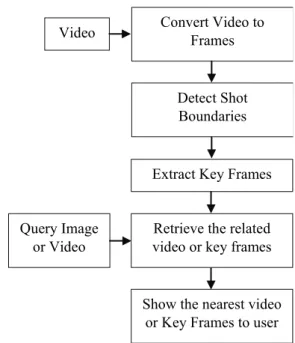
In this section, we explain the video retrieval frame-work and its steps within the following subsections. The flowchart of the proposed video retrieval method and its steps is shown in Fig. 1. First, every video is converted into frames. Second, the shot boundaries of the frames are detected. Third, the key frames of the shots are extracted. Finally, the accuracy of the proposed video retrieval system are obtained by using a query by example.

CONVERTION OF VIDEO

In this step, the videos are converted into frames, and saved into a folder to be stored. This pre-proces-sing reduces complexity and increases the speed of the proposed method in the subsequent steps (Weiming

et al., 2011).

SHOT BOUNDARY DETECTION

Shots are the basic unit of every video where a sequence of successive frames creates a video shot. All the frames in each shot usually have similar visual features such as color, texture and motion. Videos have two basic types of transitions between the shots: cut transition and gradual transition. The process of identifying between a cut and the gradual

Video Convert Video to _Frames

Detect Shot Boundaries

Extract Key Frames

Retrieve the related video or key frames Query Image

or Video

Show the nearest video or Key Frames to user

Fig. 1. The flowchart of the proposed method.

transition is called shot boundary detection. For cut transition, the dissimilarity between the last frame belonging to the current shot and the first frame of the next shot is significant. Therefore, the cut transi-tion appears immediately when viewing between the current and next shots. On the other hand, a gradual transition involves fade in, fade out, erase, object motions, camera operations and other effects. Therefore, the neighboring frames in the current and the next shot have extra visual similarities, where a gradual transition detection is more complex and confusing than a cut transition. Methods of gradual transition detection should distinguish the diversity of the mentioned effects (Cotsaces et al., 2006).

In recent years, various algorithms of shot boundary detection have been proposed such as: joint entropy, edge information, characteristics of a gradual transition, a linear transition detection (LTD) algorithm, and singular value decomposition (SVD) (Grana and Cuc-chiara, 2007; Cernekova et al., 2007; Lu ZM and Shi 2013).

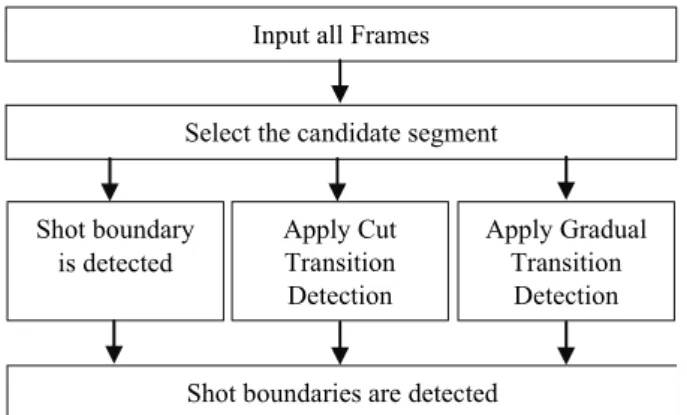
In the proposed shot boundary detection method, as seen in Fig. 2, we have adopted and modified the method used by Lu and Shi (2013). The proposed method is explained as follows:

STEP1: CANDIDATE SEGMENT

SELECTION (CSS)

length of 21 frames, and calculate the Euclidian distance between the intensity of the pixel for the first and the last frames in each segment. The intensity feature of each pixel is used because it is a mutual feature in video frames and is simple to calculate.

Input all Frames

Select the candidate segment

Shot boundaries are detected Apply Cut Transition Detection

Apply Gradual Transition

Detection Shot boundary

is detected

Fig. 2. The block diagram of the shot boundary detec-tion method.

Every calculated distance is compared to an adaptive threshold (Lu and Shi, 2013). If it is greater than the adaptive threshold, the segment is classified as a candidate segment, otherwise, that segment is re-moved. In the proposed method, the second condition which has been reported by the Lu and Shi (2013) has not been used because it is always satisfied in our dataset.

The candidate segments are refined by using a bisection-based comparison. We have combined the first and the second round bisection-based comparison of the Lu and Shi method because it reduces comple-xity and processing time. First, the Euclidian distan-ces between 1 and 11 (d1,11), 11 and 21 (d11,21), 1 and

6 (d1,6), 6 and 11 (d6,11), 11 and 16 (d11,16), 16 and 21

(d16,21) frames are obtained. Second, the calculated

distances are compared to several conditions and each candidate segment is categorized into one of four types as follows:

If (d1,11/d11,21 > 1.5 ∩d1,11/d1,21 > 0.7) ∩ (d1,6/d6,11

> 1.5 ∩d1,6/d1,11> 0.7), the shot boundary is

considered to be located in the first 6 frames. Else if (d1,11/d11,21 > 1.5 ∩d1,11/d1,21 > 0.7) ∩ (d6,11/ d1,6 > 1.5 ∩d6,11/d1,21 > 0.7), the shot boun-dary is

considered to be located in the second 6 frames. Else if (d1,11/d11,21 > 1.5 ∩d1,11/d1,21 > 0.7), it is

considered that a gradual transition may exist in the first 11 frames of the segment.

Else if (d11,21/d1,11 > 1.5 ∩d11,21/d1,21 > 0.7) ∩ (d11,16/ d16,21 > 1.5 ∩d11,16/d11,21 > 0.7), the shot boundary

is considered to be located in the third 6 frames. Else if (d11,21/d1,11 > 1.5 ∩d11,21/d1,21 > 0.7) ∩ (d16,21/

d11,16 > 1.5 ∩d16,21/d11,21 > 0.7), the shot boundary

is considered to be located in the fourth 6 frames. Else if (d11,21/d1,11 > 1.5 ∩d11,21/d1,21 > 0.7), it is

considered that a gradual transition may exist in the second 11 frames of the segment.

Else if [(d11,21/d1,11 > 1.5 ∩ d11,21/d1,21 > 0.7 ∩

(d11,16/d11,21 < 0.3 ∩ d16,21/d11,21 < 0.3)] U [(d1,11/ d11,21 > 1.5 ∩d1,11/d1,21 > 0.7) ∩ (d1,6/d1,11 < 0.3 ∩ d6,11/d1,11 < 0.3)] U [d1,11/d1,21 < 0.3 ∩d11,21/d1,21 <

0.3] this segment should be removed from the candidate segments.

Otherwise, it is considered that a gradual transi-tion may exist in the segment.

This candidate segment selection method eliminates about half of the frames in a video and many non-boundary frames. In this method, a lot of vain shot boundaries are not considered, and the rest of the shot boundaries will be used in subsequent steps. The candidate segments with 6 frames have been used to detect candidate cut transitions (CT) and candidate gradual transitions (GT) which were introduced in steps 2 and 3, respectively. The detection methods concentrate on the reduction of the required time.

STEP 2: CUT TRANSITION

DETECTION

Next, SVD is applied on matrix A. The SVD returns U, S and V vectors. The S is a vector of singular values and a diagonal matrix with the same dimension as A, with nonnegative diagonal elements in a decreasing order, and unitary matrices U and V so that A = U×S×VT_{. The 1728-dimension of the}

feature vector is reduced and mapped to 6-dimension by:

T

V

S

⋅

=

β

After obtaining β with a size of 6*6, we used the cosine distance to calculate the similarity between every two consecutive frames ft and ft–1, we choose

the cosine distance because the computational cost of the cosine distance is less than other methods which require a normalization operation. The cosine distance is quite small even for two frames having many differences. The range of the cosine distance falls in the intervals 0 to 1 which is suitable to show the similarity between two frames. The cosine distance is obtained by:

( )

(

)

j i

j i t

t f f t

β β

β β

⋅ ⋅ = Φ

=

Φ , ₋₁ , (2)

where β is calculated by Eq. 1. Meanwhile, we obtain the distance between the first and last frames in a segment with the length of 6 that is named G = Φ(f0,f5).

A cut transition in the tth _{frame will be detected if the}

following two criteria are satisfied.

G < 0.95, (3)

Φ(t) < p + (1 – p)G, (4) where t = 1, ..., 5 and p is a 0.48 (Lu ZM and Shi,

2013). The segment will be removed from the candidate segment, if the first mentioned criterion cannot be satisfied. If the first criterion in Eq. 3 can be satisfied and the second criterion in Eq. 4 cannot be satisfied, a GT detection is required, in order to ensure that, during a GT, the similarity between two consecutive frames is always much higher. In this case, the segment with a length of 6 frames is considered as the candidate GT segment with a length of 11 frames because the length of the GT segment is considered more than the CT segment.

STEP 3: GRADUAL TRANSITION

DETECTION

In this step, we use a novel method to detect the GT. The proposed GT detection method modifies the CT detection method mentioned in the previous step. This method is explained as follows:

a) The candidate GT segments which are extracted

from step 1 and added from step 2 contain 11 or typically 21 frames. In this method, in order for two frames of the different shots have a definite difference, we have added one frame before and after the candidate GT segment.

b) The HSV 3D histogram is calculated with 1728 bins for every frame in each GT candidate segment. Thus, the size of the extracted feature matrix is 1728×13 or 1728×23.

c) The SVD is applied on the feature matrix to reduce the size of the feature matrix to 10×13 or 10×23. The 1728 bins are reduced to 10 bins, such that increasing the number of bins for long segments will be more sensitive and results in more noises (Cernekova et al., 2007).

d) The distance between the first and last frames in the segment is calculated by using G = Φ(f0, fN–1)

and goes to the next sub step (sub step e) if G < 0.9. Otherwise this segment is discarded. The GT segment has a higher difference than the CT because more frames exist within the GT segment thus 0.9 is experimentally considered as the thres-hold.

e) Absolute distance difference, d(t) = Φ (fs, ft) –

Φ (ft, fe), (t = 0, …, 10 or 20), is calculated where

fs and fe stand for the last frame of the previous

shot and the first frame of the next shot, respectively. If the criterion max(d(t)) – min(d(t)) > 0.33 is satisfied, go to the next sub step (sub step f). Otherwise this segment is discarded and go to the first sub step (sub step a).

f) Criterion |(tm – (N + 1)/2)/N| ≤ 0.25 is checked

where tm is the point with the minimum value of

the absolute distance difference, d, and N = 11 or 21. If it is satisfied, the criterion (KL + KR)/ N≤ 0.3 will be checked where KL and KR are the number of the ascending points before tm and the number of the descending points after tm, respec-tively. If it is satisfied, the candidate GT segment is considered as a GT segment. Otherwise the candidate GT segment is considered as a CT seg-ment. If the Criterion |(tm – (N + 1)/2)/N| ≤ 0.25 is

not satisfied, the position of the segment should be adjusted and moved L frames backwards or forwards which is obtained by L = tm – ((N + 1)/2)

and go to the first sub step.

video dataset will show that the proposed scheme can provide high accuracy and speed to detect both abrupt and gradual transitions.

KEY FRAME EXTRACTION

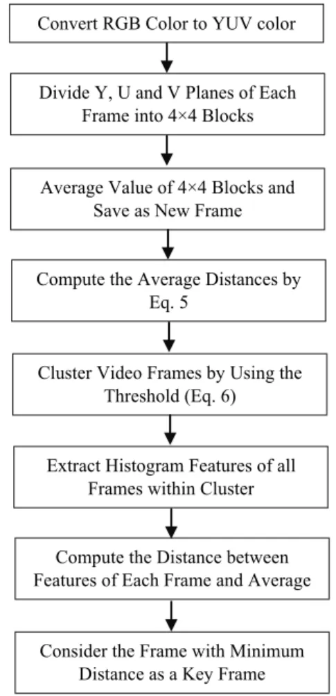
The shot boundaries of the video are detected by the mentioned algorithm which is described in the shot boundary detection section. In this section, a key frames extraction method is described. These frames are extracted by using an unsupervised clustering method. The color features of the videos have been used in the shot boundary detection step, but the video motion has not been considered as a feature. Motion is a special feature of a video that distinguishes a video from an image. Video motion is classified to the foreground motion and the background motion that are created by moving an object and a camera, respectively. The camera movements include tilting up or down, zooming in or out and panning left or right. Due to the camera movements, moving objects and lightning changes, consecutive frames within the same shot have visual content differences. These dif-ferences are obtained and extracted by using motion compensation methods (Wolf, 1996). In this paper, the motion compensation procedure is employed by using a block-matching method. The key frame extraction method is shown in Fig. 3 and performed as follows.

In the key frame extraction method, the YUV color space is used instead of the RGB color space because it provides better results in our experiment. Therefore, first, the RGB images are converted to YUV images. Second, each frame is divided into 4×4 blocks without any overlapping blocks by using the motion feature. The average value of the 4×4 blocks is obtained and saved as a new image (frame) thus the size of the original image is reduced. This process is performed for every Y, U and V planes of the frames. The average of distances (AD) between new Y, U, and V planes of consecutive frames is obtained by,

AD = average (|Yave (k) – Yave (k – 1)| + |Uave (k) – Uave (k – 1)| + |Vave (k) – Vave (k – 1)|). (5)

Third, we cluster video frames by using AD values which are obtained for all consecutive frames within the shot. The cluster boundary is obtained by comparing the normalized AD values to a threshold T,

T AD Maximum

AD _>

)

( , (6)

where T is set as 0.95. This value is based on providing the best performance in our experiments.

Clustering algorithms use a threshold parameter to control the density of the clustering. The low value for the threshold T increases the number of clusters and key frames, but a threshold should be adjusted to be suitable for various videos.

Convert RGB Color to YUV color

Divide Y, U and V Planes of Each Frame into 4×4 Blocks

Average Value of 4×4 Blocks and Save as New Frame

Compute the Average Distances by Eq. 5

Cluster Video Frames by Using the Threshold (Eq. 6)

Extract Histogram Features of all Frames within Cluster

Consider the Frame with Minimum Distance as a Key Frame Compute the Distance between Features of Each Frame and Average

Fig. 3. The block diagram of the key frame extraction method.

After clustering, we use the histogram feature to extract a key frame within a cluster. The histogram counts the number of pixels within the sets of the defined bins, which allows it to reduce the complexity and calculation time. The histogram with 64 bins of the Y plane of the prior image (frame) is considered as a feature of the frame. 64 bins are usually adequate the histogram feature for accurate results (Shuping and Xinggang, 2005). The histogram feature of all frames within a cluster are extracted. Then, the distances between the histogram feature of each frame and the average of the histogram feature of the frames within the cluster are obtained. A frame with a minimum distance can be considered as a key frame because it is closest to a cluster centroid.

RETRIEVAL ALGORITHM

the CBIR methods to achieve the CBVR system. The key frames of a video are extracted by the previous subsection and stored in a folder. The main purpose of the proposed video retrieval system is to retrieve relevant key frames. The S and I planes of the HSI color space are used to extract texture features of the frames. The discrete wavelet transform (DWT), as the texture feature, is used in the proposed method (Mohamadzadeh and Farsi, 2014). We use the approximation components in the proposed method because the wavelet transform analyses the signal at various frequency bands. The low-low frequency component provides a coarse scale approximation of the image, while the other frequency components fill in the detail and extract edges. In previous steps, we have proposed and modified new algorithms for the shot boundary detection and the key frame extraction. In the following, we propose and compare the retrieval methods via sparse representation and Intensity-HDWT (Farsi and Mohamadzadeh, 2013).

The sparse representation

Most coefficients of the DWT are small when we compute a wavelet transform of a typical natural image. Hence, we can obtain an accurate approximation of the image by setting the small coefficients to zero, or thresholding the coefficients, to obtain a sparse representation (Mohamadzadeh and Farsi, 2014). In this paper, the DWT is applied on the S plane in the HSI color space of the approximation component of the DWT output and this process is repeated five times. The extracted feature using this procedure is called the Iterative DWT (IDWT) feature.

We review some fundamentals in the sparse representations and then we explain our proposed method for the video retrieval application using sparse representation. The concatenation of two vectors is written by:

[

]

[

] [

]

2 1 2

1; _x ; x,x x x

x x

x _⎥ =

⎦ ⎤ ⎢ ⎣ ⎡

= . We represent

l0–norm by ⋅ 0, l1–norm by ⋅ 1and the Euclidean or

l2–norm by ⋅ 2. Given a signal vector b∈R

m_{, signal}

(or atomic) decomposition is the linear combination of n basic atoms ai∈Rm, (1 ≤i≤n) which constructs

the signal vector b[n] as:

b = a1x1 + a2x2 + ⋅⋅⋅ + anxn = Ax, (7)

where A = [a1, a2, ..., an], x = (x1, x2, ..., xn),

Dictionary A comprises n signals [a1, a2, ..., an]

called atoms. In the Discrete Fourier Transform (DFT) or the classical signal decomposition, the number of atoms (n) is equal to the length of signals (m), where a unique solution exists for this problem.

However, when these two parameters are not equal, or in other words when n > m, the decomposition is not unique. Sparse decomposition aims to seek for a solution in which as few atoms as possible would contribute in the decomposition. This is equivalent to seeking the sparsest solution of the undetermined system of linear equation b = Ax. We seek the spar-sest solution for this equation by solving the optimi-zation problem (Elad, 2012). In recent years, several development algorithms have been reported to solve Eq. 7 such as Smoothed L0 (SL0), Dual Augmented Lagrangian Method (DALM), Primal Augmented Lagrangian Method (PALM) and Homotopy method (Elad, 2012; Yang et al., 2012). In this paper, we use DALM, SL0, Homotopy, and PALM algorithms to solve Eq. 7 because these algorithms provide better performance and lower processing time than other algorithms (Yang et al., 2012). We use these algorithm to investigate the sparse representation and to find its usefulness in the video retrieval application. Therefore, we apply the following algorithm via sparse represen-tation to achieve the desired video retrieval.

1. In the video retrieval literature, we construct the dictionaryA_{by using sufficient training samples}

of the ith _{image, A}

i = [νi,1; νi,2;...; νi,m] ∈Rm×1,

where νi,j represents the jth feature of the ith

extracted image by applying the IDWT method on the image. Therefore,

A = [A1, A2,..., An] ∈Rm×n. (8)

2. Extract the feature vector of the query image by applying the IDWT method, b ∈Rm_.

3. Seek sparse representation, x0∈Rn, by solving

Eq. 7 and using DALM, SL0, Homotopy, and PALM techniques. Therefore, some elements of

x0 are zero except those associated with the kth

class.

4. Separate elements of A and x0 into k clusters,

{ {

0 1 2 0,1 0,2 0,

1 2

; ; ; _j ; ; ; _n ; ; ; _k

k

x =⎡⎢α α α α ⎤⎥ ⎡=_⎣x x x ⎤_⎦

⎢ ⎥

⎣14243K K K K ⎦ K

, (9)

{ {

[

]

1 2 1 2

1 2

, , , _j , , , _n , , , _k

k

A A A A D D D

A=⎡⎢ ⎤⎥=

⎢ ⎥

⎣14243K KKK ⎦ K

. (10)

5. Define Ck = Dkx0,k∈Rmby using the distinguished

elements in the previous step.

6. Compute the Euclidean Distance (ED) between the feature vector of the query image (b) and Ck

(

)

m

k i i

i

ED b C

=

=

∑

7. Compute the weighting of the elements of x0 by

considering the ED and Eq. 10

0,1 0,2 0,

; ; ;

1 2

n R

x

x x _k

xweighted _{ED ED}

EDk ∈

=⎡⎢ ⎤⎥

⎢ ⎥

⎣ K ⎦

. (12)

8. Finally, the best relevant key frames are retrieved by using the sorted element of xweighted.

Intensity-HDWT method

In this paper, we used the Hadamard matrix and Discrete Wavelet Transform (HDWT) method to achieve the CBVR (Farsi and Mohamadzadeh, 2013). The Intensity plane of the proposed method provides an acceptable performance and the size of the feature vector is satisfactory. The features of the key frames and a query are extracted by using the HDWT. Then, the Euclidian distance between the key frames feature and the query feature is calculated, and the related key frames or videos according to the user’s request are shown. The size of the feature vector of the Hue-Maximum-Minimum-Difference (HMMD) color space is three times bigger than the Intensity, therefore, we use the Intensity plane instead of the HMMD planes because the size of the feature vector plays an important role in the proposed method. The HDWT method has been briefly explained as below (Farsi and Mohamadzadeh, 2013).

1. Apply the DWT on the Intensity plane with a size of N×N to generate the approximation (Low-Low), the horizontal (Low-High), the vertical (High-Low) and the diagonal (High-High) com-ponents.

2. Construct the modified approximation components by multiplying the actual approximation compo-nents and the Hadamard matrix with the size of the approximation component. The Hadamard ma-trices are the square mama-trices whose entries are either +1 or −1, and their rows are mutually ortho-gonal.

3. Construct the modified plane from step 2 by applying the inverse wavelet transform with the modified approximation components, the zeroing horizontal, the vertical and the diagonal compo-nents. The new image is used in the next level to construct the new approximation components. 4. Take the alternative rows and columns by

down-sampling the output from step 3 with a size of N/2×N/2. The down-sampling reduces the size of

the feature vector which is important for increa-sing speed of the retrieval.

5. Construct the HDWT feature of the level-p by repeating steps 2 to 4, ‘p’ times on the each plane. 6. Use the approximation components of the level-p. this results in step 2 as the HDWT feature of the level-p.

We generated the feature vectors of the data set image by applying the HDWT level-5 and stored the approximation component as the feature vectors for each image.

RESULTS

EVALUATION MEASURES

In order to evaluate the performance of the pro-posed retrieval systems, we use two evaluation metrics. Farsi and Mohamadzadeh (2013) proposed a method using the combination of precision and recall criteria as performance measures for the CBIR and CBVR systems. The precision and recall criteria are given by Eq. 13 and Eq. 14, respectively.

_ _ _ _

_ _ _ _

Number of Relevant Images Retrieved Precision

Total Number of Images Retrieved

=

, (13)

_ _ _ _

_ _ _ _ _ _

Number of Relevant Images Retrieved Recall

Total Number of Relevant Images in Database

=

. (14) According to Farsi and Mohamadzadeh (2013), P(1) has been adopted, with precision at 100% recall (i.e., precision after retrieving all of the relevant documents). P(1) is number of relevant images divi-ded by the total number of images that are retrieved. This becomes the fraction of retrieved images that are relevant to the query image. We use this value beca-use precision and recall are considered to be related to each other and are meaningless if taken separately.

DATASETS

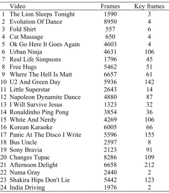
U2 and green day, Little superstar, Napoleon dynamite dance, I will survive Jesus, Ronaldinho ping pong, White and nerdy, Korean karaoke, Panic at the disco I write, Bus uncle, Sony Bravia, Changes Tupac, Afternoon delight, Numa gray, Shakira hips don't lie, and India driving. We have selected 24 videos to achieve the video retrieval and to compare the methods (Wu et al., 2009). These videos include the RGB frames with a size of 320×240. Therefore, the size of the feature vector in level 5 of HDWT and IDWT is 80 features. As described in the previous sections, first, the shot boundaries are detected, second, the key frames are extracted, and finally, the retrieval methods are applied to the dataset. We have proposed and modified the new methods for each part. The results of the retrieval system is shown in the next step.

INDEXING RESULTS

In this section, we represented the results of the proposed method and compared them to other methods. The P(1) metric is obtained to compare and evaluate the proposed method using different accele-ration algorithms. The best scores for each video category are bolded. The name of each video cate-gory, the number of frames and the number of key frames are shown in Table 1. These key frames are extracted by the proposed method which has been described in the key frame extraction section.

Table 1. The name of videos, the number of frames and key frames.

Video Frames Key frames

1 The Lion Sleeps Tonight 1590 3 2 Evolution Of Dance 8950 4

3 Fold Shirt 557 6

4 Cat Massage 650 4

5 Ok Go Here It Goes Again 4603 4

6 Urban Ninja 4631 106

7 Real Life Simpsons 1796 45

8 Free Hugs 5462 51

9 Where The Hell Is Matt 6657 61 10 U2 And Green Day 5936 142 11 Little Superstar 2643 14 12 Napoleon Dynamite Dance 4880 87 13 I Will Survive Jesus 1323 32 14 Ronaldinho Ping Pong 3854 36 15 White And Nerdy 4269 106

16 Korean Karaoke 6005 66

17 Panic At The Disco I Write 5596 155

18 Bus Uncle 2597 8

19 Sony Bravia 2123 91

20 Changes Tupac 8286 109

21 Afternoon Delight 6658 212

22 Numa Gray 2440 2

23 Shakira Hips Don't Lie 5442 123

24 India Driving 1976 2

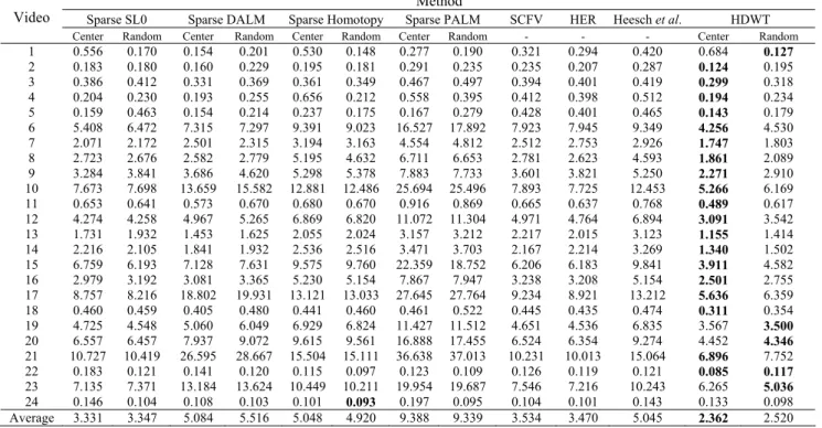
In Table 2, the experimental results of the pro-posed methods via Intensity-HDWT, spars DALM, sparse SL0, sparse Homotopy, sparse PALM, and HER (Li et al., 2015), Heesch et al. (2004) and SCFV (Araujo et al., 2015) methods in the CC_WEB_ VIDEO dataset have been shown. In this experiment, the best performance rate for the proposed method via Intensity-HDWT with the center or random queries is being tested. In comparing the performances, the P(1) of the proposed method via Intensity-HDWT, sparse SL0, sparse DALM sparse Homotopy, sparse PALM, HER, Heesch et al. (2004), and SCFV methods values fall in the intervals [40.91, 100], [7.69, 100], [15.38, 100], [13.33, 100], [9.09, 100], [23.08, 98.76], [15.38, 90.2], and [21.23, 95.67] respectively. The average is calculated by taking the mean value of the P(1) from the video categories. The average of the P(1) of the proposed method via Intensity-HDWT with center query is 84.82%. After the proposed method via Intensity-HDWT with center query, the propose method via Intensity-HDWT with the random query provides better performance than the other methods.

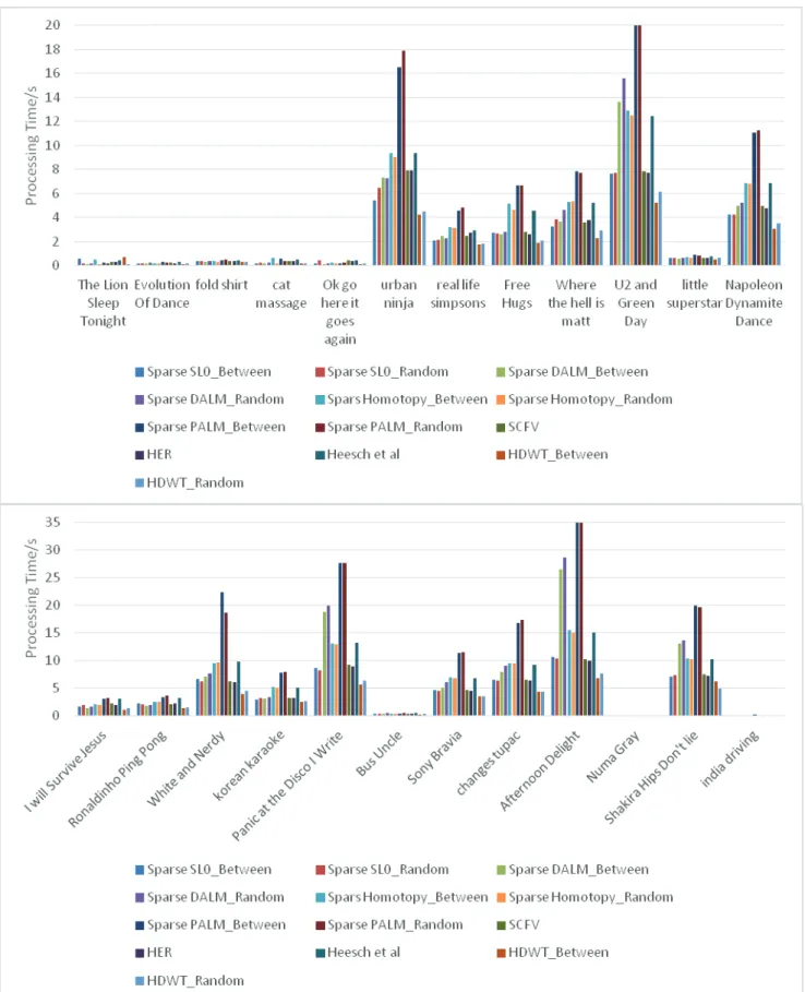
The processing times of the proposed methods in the CC_WEB_VIDEO dataset are obtained and shown in Table 3. Once again, the proposed methods via Intensity-HDWT with the center and random queries provide the best processing times. Meanwhile, the average processing time of the proposed methods via Intensity-HDWT with center query is less than the other methods.

In the Changes Tupac video (video: 20), the sparse Homotopy with the random query provides a better performance than the other methods (P(1) = 60.87%), but the processing time of the sparse Homo-topy with the random query is 9.561 seconds. Whereas, the pro-cessing time of the proposed method via In-tensity-HDWT with the random query is 4.346 seconds and the P(1) is equal to 58.7%. Therefore, in considering the P(1) and the processing time, the proposed method via Intensity-HDWT provides better performance than other methods.

All numerical experiments are performed on a personal computer with a 2.6 GHz Core i5 and 3.8 Gb of Ram. This computer runs on Windows 7, with MATLAB 7.01 and a VC++ 6.0 compiler installed.

Table 2. The P (1)% of the proposed methods in each video. Method

Sparse SL0 Sparse DALM Sparse Homotopy Sparse PALM SCFV HER Heesch _al. et HDWT Video

Center Random Center Random Center Random Center Random - - - Center Random

1 100 100 100 100 100 100 100 100 84.12 97.78 75.73 100 100

2 100 100 100 100 100 100 100 100 93.3 97.44 80.44 100 100

3 100 100 100 100 100 100 100 100 88.3 98.76 82.87 100 100

4 100 100 100 100 100 100 100 100 79.2 94.33 78.69 100 100

5 100 100 100 100 100 100 100 100 82.4 90.12 85.22 100 100

6 65.12 46.51 67.44 55.82 72.09 69.77 69.77 60.46 51.53 55.82 45.76 93.03 72.09

7 56.25 31.25 50 25 62.50 37.5 56.25 25 37.5 50 32.23 75 62.5

8 31.82 40.91 22.73 22.72 36.36 50 27.27 9.09 25.48 27.27 22.72 40.91 59.09

9 75 75 75 75 85.71 71.43 75 78.57 75 75 71.43 89.29 82.14

10 42.86 47.62 42.86 44.44 49.21 53.97 39.68 42.86 44.44 48.23 41.34 63.49 58.73

11 100 100 100 100 80 100 100 100 80 80 80 100 100

12 45.45 57.58 45.45 45.45 75.76 75.76 57.57 48.48 45.45 45.45 45.45 75.76 75.76 13 15.38 7.69 15.38 23.08 30.77 30.77 23.08 38.46 21.23 23.08 15.38 92.31 92.31 14 20 46.66 26.67 40 13.33 40 26.67 33.33 40 42.22 36.93 66.67 60 15 69.39 65.31 69.39 63.22 67.35 81.63 71.42 67.35 63.22 65.31 61.22 79.59 81.63

16 32 36 32 24 48 52 28 28 28 32 24 80 68

17 66.15 61.54 67.69 64.62 75.38 67.69 72.30 75.38 66.15 67.69 63.45 76.92 78.46

18 100 75 100 50 100 50 100 100 50 75 50 100 100

19 56.25 59.38 53.13 53.13 78.12 75 62.5 62.5 48.13 53.13 45.12 84.38 90.63

20 36.96 50 36.96 34.78 54.35 60.87 34.78 36.96 34.78 36.96 30.15 50 58.7 21 72.06 77.94 70.59 82.35 79.41 79.41 75 75 58.76 60.23 55.43 85.3 80.88

22 100 100 100 100 100 100 100 100 95.67 97.23 88.56 100 100

23 56.6 56.6 58.49 54.72 66.04 67.92 62.26 67.92 50.46 56.6 48.45 83.02 77.36

24 100 100 100 100 100 100 100 100 90.22 95.23 90.2 100 100

Average 68.39 68.13 68.07 64.93 74.44 73.49 70.06 68.73 59.72 65.20 56.28 84.82 83.26

Table 3. The processing times (second) of the proposed methods in each video. Method

Sparse SL0 Sparse DALM Sparse Homotopy Sparse PALM SCFV HER Heesch et al. HDWT Video

Center Random Center Random Center Random Center Random - - - Center Random 1 0.556 0.170 0.154 0.201 0.530 0.148 0.277 0.190 0.321 0.294 0.420 0.684 0.127

2 0.183 0.180 0.160 0.229 0.195 0.181 0.291 0.235 0.235 0.207 0.287 0.124 0.195 3 0.386 0.412 0.331 0.369 0.361 0.349 0.467 0.497 0.394 0.401 0.419 0.299 0.318 4 0.204 0.230 0.193 0.255 0.656 0.212 0.558 0.395 0.412 0.398 0.512 0.194 0.234 5 0.159 0.463 0.154 0.214 0.237 0.175 0.167 0.279 0.428 0.401 0.465 0.143 0.179 6 5.408 6.472 7.315 7.297 9.391 9.023 16.527 17.892 7.923 7.945 9.349 4.256 4.530 7 2.071 2.172 2.501 2.315 3.194 3.163 4.554 4.812 2.512 2.753 2.926 1.747 1.803 8 2.723 2.676 2.582 2.779 5.195 4.632 6.711 6.653 2.781 2.623 4.593 1.861 2.089 9 3.284 3.841 3.686 4.620 5.298 5.378 7.883 7.733 3.601 3.821 5.250 2.271 2.910 10 7.673 7.698 13.659 15.582 12.881 12.486 25.694 25.496 7.893 7.725 12.453 5.266 6.169 11 0.653 0.641 0.573 0.670 0.680 0.670 0.916 0.869 0.665 0.637 0.768 0.489 0.617 12 4.274 4.258 4.967 5.265 6.869 6.820 11.072 11.304 4.971 4.764 6.894 3.091 3.542 13 1.731 1.932 1.453 1.625 2.055 2.024 3.157 3.212 2.217 2.015 3.123 1.155 1.414 14 2.216 2.105 1.841 1.932 2.536 2.516 3.471 3.703 2.167 2.214 3.269 1.340 1.502 15 6.759 6.193 7.128 7.631 9.575 9.760 22.359 18.752 6.206 6.183 9.841 3.911 4.582 16 2.979 3.192 3.081 3.365 5.230 5.154 7.867 7.947 3.238 3.208 5.154 2.501 2.755 17 8.757 8.216 18.802 19.931 13.121 13.033 27.645 27.764 9.234 8.921 13.212 5.636 6.359 18 0.460 0.459 0.405 0.480 0.441 0.460 0.461 0.522 0.445 0.435 0.474 0.311 0.354 19 4.725 4.548 5.060 6.049 6.929 6.824 11.427 11.512 4.651 4.536 6.835 3.567 3.500

20 6.557 6.457 7.937 9.072 9.615 9.561 16.888 17.455 6.524 6.354 9.274 4.452 4.346

21 10.727 10.419 26.595 28.667 15.504 15.111 36.638 37.013 10.231 10.013 15.064 6.896 7.752 22 0.183 0.121 0.141 0.120 0.115 0.097 0.123 0.109 0.126 0.119 0.121 0.085 0.117

23 7.135 7.371 13.184 13.624 10.449 10.211 19.954 19.687 7.546 7.216 10.243 6.265 5.036

24 0.146 0.104 0.108 0.103 0.101 0.093 0.197 0.095 0.104 0.101 0.143 0.133 0.098 Average 3.331 3.347 5.084 5.516 5.048 4.920 9.388 9.339 3.534 3.470 5.045 2.362 2.520

Consequently, as shown in Tables 1 and 2, and Figs. 4 and 5, the proposed method via Intensity-HDWT provides better performance than other methods. The obtained results show that with respect to the performance rate and the size of the feature vectors, the proposed method scores extremely well.

CONCLUSIONS

In this paper, we proposed a new method for video retrieval via Intensity-HDWT. The aim of the proposed algorithm is to provide a CBVR technique by using the new shot detection method, the new key frame extraction method, and the HDWT feature. The HSI and YUV color spaces have been considered. The P(1) metric for the proposed method and the other methods has been computed and compared. The CC_WEB_VIDEO dataset has been used to obtain this metric. Experimental results for this dataset showed that the proposed method via the Intensity-HDWT algorithm yields higher retrieval accuracy than the other methods with no greater feature vector size. In addition, the proposed method provided a higher performance gain in both the P(1) metric and processing time over the other methods for the 24 videos of the CC_WEB_VIDEO dataset. Moreover, the proposed system both reduces the size of the feature vector, the storage space, the processing time and improves the video retrieval performance. For future work, it is proposed to use video query instead of frame query.

REFERENCES

Adcock J, Girgensohn A, Cooper M, Liu T, Wilcox L, Rieffel E (2004). FXPAL experiments for TRECVID 2004. In Proc TREC Video Retrieval Evaluation, Gai-thersburg, MD (February 17, 2005) Available: http:// www-nlpir.nist.gov/projects/tvpubs/tvpapers04/fxpal.pdf Amir A, Hsu W, Iyengar G, Lin CY, Naphade M, Natsev

A, et al. (2003). IBM research TRECVID-2003 video retrieval system. In Proc TREC Video Retrieval Evalu-ation, Gaithersburg, MD (June 15, 2004) Available: http://www-nlpir.nist.gov/projects/tvpubs/tvpapers03/ ibm.smith.paper.final2.pdf

Araujo A, Chaves J, Angst R, Girod B (2015). Temporal aggregation for large-scale query-by-image video retrie-val. Proc ICIP, Stanford University, CA.

Calic J, Izquierdo E (2002). Efficient key-frame extraction and video analysis. In Proc Int Conf Inf Technol: Coding Computer 28–33.

Camara-Chavez G, Precioso F, Cord M., Phillip-Foliguet S, Araujo A. (2007). Shot boundary detection by a hierarchical supervised approach. In Proc Int Conf Syst, Signals Image Processing 197–200.

Cernekova Z, Pitas I, Nikou C (2006). Information theory-based shot cut/fade detection and video summarization. IEEE T Circ Syst Vid 16:82–90.

Cernekova Z, Kotropoulos C, Pitas I (2007). Video shot-boundary detection using singular-value decomposition and statistical tests. J Electron Imaging 16:043012-1– 043012-13.

Chung YY, Chin WKJ, Chen X, Shi DY, Choi E, Chen F (2007). Content-based video retrieval system using wavelet transform. WSEAS T Circ Syst 6:259–65. Chang Y, Lee DJ, Hong Y, Archibald J (2008).

Unsuper-vised video shot detection using clustering ensemble with a color global scale invariant feature transform descriptor. Eurasip J Image Vid 1–10.

Cooke E, Ferguson P, Gaughan G, Gurrin C, Jones G, Borgue HL, Lee H, et al. (2004). TRECVID 2004 experiments in Dublin city university, in Proc TREC Video Retrieval Eval, Gaithersburg, MD (February 17, 2005) Available: http://wwwnlpir.nist.gov/projects/ tvpubs/tvpapers04/dcu.pdf

Cotsaces C, Nikolaidis N, Pitas I (2006). Video shot de-tection and condensed representation. A review. IEEE Signal Proc Mag 23:28–37.

Damnjanovic U, Izquierdo E, Grzegorzek M (2007). Shot boundary detection using spectral clustering. In Proc Eur Signal Process Conf, Poznan, Poland, 1779–83. Elad M (2012), Sparse and redundant representations,

Springer, New York.

Farsi H, Mohamadzadeh S (2013). Colour and texture feature-based image retrieval by using Hadamard matrix in discrete wavelet transform. IET Image Process 7:212–8. Ferman AM, Tekalp AM (2003). Two-stage hierarchical

video summary extraction to match low-level user browsing preferences. IEEE T Multimedia 5:244–56. Gargi U, Kasturi R, Strayer SH (2000). Performance

cha-racterization of video-shot-change detection methods. IEEE T Circ Syst Vid 10:1–13.

Grana C, Cucchiara R (2007). Linear transition detection as a unified shot detection approach. IEEE T Circ Syst Vid 17:483–9.

Guironnet M, Pellerin D, Guyader N, Ladret P (2007). Video summarization based on camera motion and a subjective evaluation method. Eurasip J Image Video Processing 2007:1–12.

Hauptmann A, Chen MY, Christel M, Huang C, Lin WH, Ng T, et al. (2004). Confounded expectations: Infor-media at TRECVID 2004. In Proc TREC Video Retrieval Evaluation, Gaithersburg, MD, (February 17, 2005) Available: http://www-nlpir.nist.gov/projects/tvpubs/ tvpapers04/cmu.pdf

Heesch D, Pickering M, Yavlinsky A, Rüger S (2004). Video retrieval within a browsing framework using key frames. In: Proc TREC video. NIST, Gaithersburg. Hoi CH, Wong LS, Lyu A (2006). Chinese university of

Hong Kong at TRECVID 2006: Shot boundary detection and video search. In Proc TREC Video Retrieval Evaluation, Available: http://wwwnlpir.nist.gov/projects/ tvpubs/tv6.papers/chinese_uhk.pdf

Lew MS, Sebe N, Djeraba C, Jain R (2006). Content-based multimedia information retrieval: State of the art and challenges. ACM T Multim Comput 2:1–19.

Li Y, Wang R, Huang Z, Shan S, Chen X (2015). Face video retrieval with image query via hashing across Euclidean space and Riemannian manifold. Computer Vision and Pattern Recognition (CVPR), 2015 IEEE Conference on, 4758-67.

Liu T, Zhang X, Feng J, Lo K (2004). Shot reconstruction degree: A novel criterion for key frame selection. Pattern Recogn Lett 25:1451–7.

Lu H, Tan YP (2005). An effective post-refinement method for shot boundary detection. IEEE T Circ Syst Vid 15:1407–21.

Lu ZM, Shi Y (2013). Fast Video Shot Boundary Detection Based on SVD and Pattern Matching. IEEE T Image Process 22:5136-45.

Matsumoto K, Naito M, Hoashi K, Sugaya F (2006). SVM-based shot boundary detection with a novel feature. In Proc. IEEE Int Conf Multimedia Expo 1837–40. Mohamadzadeh S, Farsi H (2014). Image retrieval using

color-texture features extracted from Gabor-Walsh wavelet pyramid. Journal of Information Systems and Telecommunication 2:31-40.

Montagna R, Finlayson GD (2012). Padua point interpolation and Lp-Norm minimization in color-based image indexing and retrieval. IET Image Process 6:139-47. Mukherjee DP, Das SK, Saha S (2007). Key frame estimation

in video using randomness measure of feature point pattern. IEEE T Circ Syst Vid 7:612–20.

Narasimha R, Savakis A, Rao RM, De Queiroz R (2003). Key frame extraction using MPEG-7 motion descriptors. In Proc Asilomar Conf Signals, Syst Computer 2:1575–9. Porter SV (2004). Video segmentation and indexing using motion estimation. Ph.D. dissertation, Dept. Computer and Science, Univ Bristol, Bristol, U.K.

Schoeffmann K, Hopfgartner F, Marques O, Boeszoermenyi L, Jose JM (2010). Video browsing interfaces and applications: A review. SPIE Rev 1(1): 018004.1–35. Shuping Y, Xinggang L (2005). Key frame extraction using

unsupervised clustering based on a statistical model. Tsinghua Sci Technol 10:l69-173

Smeaton SF, Over P, Doherty AR (2010). Video shot boun-

dary detection: Seven years of TRECVid activity. Comput Vis Image Und 114:411–8.

Snoek CGM, Worring M, Koelma DC, Smeulders AWM (2007). A learned lexicon-driven paradigm for inter-active video retrieval. IEEE T Multimedia 9:280–92. Song XM, Fan GL (2006). Joint key-frame extraction and

object segmentation for content-based video analysis. IEEE T Circ Syst Vid 16:904–14.

Truong BT, Venkatesh S (2007). Video abstraction: A systematic review and classification. ACM T Multim Comput 3:1–37.

Wang T, Wu Y, Chen L (2007). An approach to video key-frame extraction based on rough set. In Proc Int Conf Multimedia Ubiquitous Eng.

Weiming, Hu, Nianhua, Xie, Li Li, Xianglin Zeng, May-bank S (2011). A survey on visual content-based video indexing and retrieval. IEEE T Syst Man Cy C 41:11-22

Wolf W. (1996). Key frame selection by motion analysis. In Proc IEEE Int Conf Acoust, Speech and Signal Proc Atlanta, GA, USA, 2:1228-31.

Wu X, Ngo CW, Hauptmann AG, Tan H (2009). Real-time near-duplicate elimination for web video search with content and context. IEEE T Multimedia 11:196-207. Xiong Z, Zhou XS, Tian Q, Rui Y, Huang TS (2006).

Semantic retrieval of video review of research on video retrieval in meetings, movies and broadcast news, and sports. IEEE Signal Proc Mag, 23(2): 18–27.

Yang AY, Zhou Z, Ganesh A, Sastry SS, Yi Ma (2012). Fast l1-minimization algorithms for robust face reco-gnition. arXiv:1007.3753v4 [cs.CV].

Yan R, Hauptmann AG (2007). A review of text and image retrieval approaches for broadcast news video. Inform Retrieval 10:445–84.

Yuan J, Wang H, Xiao L, Zheng W, Li J, Lin F, Zhang B (2007). A formal study of shot boundary detection. IEEE T Circ Syst Vid 17:168–86.

Yu XD, Wang L, Tian Q, Xue P (2004). Multilevel video representation with application to key frame extraction. In Proc Int Multimedia Modelling Conf 117–23. Zhang XD, Liu TY, Lo KT, Feng J (2003). Dynamic