A COMBINATORIAL PROCEDURE FOR CONSTRUCTING D-OPTIMAL EXACT DESIGNS
I.B. Onukogu, M.P. Iwundu
1. INTRODUCTORY REMARKS
The subject of constructing optimal N-point exact designs for response sur-faces is one that has received research attention over the last half century. For some polynomial and trigonometric response functions defined in regular geo-metric spaces, it is possible to determine optimal designs algebraically; see, e.g. Federov (1972, ch. 3), Pazman (1986; ch. V, VI). In 2n central composite factorial
experiments, optimal designs can be obtained analytically for second order re-sponse surfaces; see, Box and Draper (1951), Onukogu (1997; ch. 4).
However, in more general settings, analytical solutions become intractable and iterative methods come into consideration; see the variance – exchange algorithm in Mitchell (1974), Atkinson and Donev (1992, ch. 13), and Pazman (1986). Un-fortunately, many iterative methods are not guaranteed to reach the global opti-mum or they reach it rather slowly.
Under the present procedure the support points that make up the space iX are grouped into H concentric balls,
1 2
11 21 1
12 22 2
1 2
1 2
, ,..., ,
... ... ...
H H
H H
n n Hn
x x x
x x x
g g g
x x x
⎛ ⎞ ⎛ ⎞ ⎛ ⎞
⎜ ⎟ ⎜ ⎟ ⎜ ⎟
⎜ ⎟ ⎜ ⎟ ⎜ ⎟
=⎜ ⎟ =⎜ ⎟ =⎜ ⎟
⎜ ⎟ ⎜ ⎟ ⎜ ⎟
⎜ ⎟ ⎜ ⎟ ⎜ ⎟
⎝ ⎠ ⎝ ⎠ ⎝ ⎠
such that,
hk
x , a constant for all k=1, 2,..., nh (1)
hk
x is an n-component vector of support points in X, h = 1, 2, ..., H; k = 1, 2,
..., nh and d1>d2...>dH; 1 H
h h=
n =N
At any point j in the sequence, a set of design measures ξN is specified by an H-tuple, ( , , r1j r2j ..., )rHj ; where rhj is the number of support points to be taken from ball h;
1
H hj, hj 0. h
N r r
=
=
∑
≥Therefore, each design measure ξN is a composite of the sub-measures from the different balls;
1
2
... N
H ξ ξ ξ
ξ
⎛ ⎞ ⎜ ⎟ ⎜ ⎟ =
⎜ ⎟ ⎜ ⎟ ⎝ ⎠ .
Also, the number of available designs at the jth step is aj =a1j⋅a2j ⋅ ⋅... aHj;
where ahj is the number of available designs from the hth ball. These numbers can be easily computed; for example, if selection of support points from the hth all is without replacement,
!
!( )!
h h
hj
hj hj h hj
n n
a
r r n r
⎛ ⎞ = ⎜ ⎟ =
−
⎝ ⎠ .
The combinatorial procedure strives to reach the D-optimal design by
1) minimizing the number of determinantal evaluations needed to be made in the set of aj available designs, and
2) minimizing the number of steps required to convergence.
2. EQUIVALENCE OF DESIGNS
Let M( )ξ1 and M( )ξ2 be two non-singular p p× information matrices, then:
1 2
det( ( )) M ξ > det( ( ))M ξ ⇒ ξ1 is better than ξ2.
1 2
det( ( )) M ξ = det( ( ))M ξ ⇒ξ1 is equivalent to ξ2.
For more discussions on the equivalence of designs see, for example Pazman (1986), Onukogu (1997).
equal diagonal elements in their information matrices. This means for instance that if ξ11, , ξ12 ..., ξ1p and ξ21, , ξ22 ..., ξ2q are the sub-design measures from balls one and two respectively, then the N-points composite designs; namely,
1
11 12 1 11
2
21 21 21 22
... p ... p q ξ
ξ ξ ξ ξ
ξ
ξ ξ ξ ξ
⎛ ⎞
⎛ ⎞⎛ ⎞ ⎛ ⎞⎛ ⎞
⎜ ⎟
⎜ ⎟⎜ ⎟ ⎜ ⎟⎜ ⎟
⎝ ⎠⎝ ⎠ ⎝ ⎠⎝ ⎠ ⎝ ⎠
can be grouped into q sets:
11 12 1
11 12 1 11 12 1
2 2 2
21 21 21 22 22 22
... p ; ... p ; ...; ... p
q q q
ξ ξ ξ
ξ ξ ξ ξ ξ ξ
ξ ξ ξ
ξ ξ ξ ξ ξ ξ
⎛ ⎞⎛ ⎞ ⎛ ⎞
⎛ ⎞⎛ ⎞ ⎛ ⎞ ⎛ ⎞⎛ ⎞ ⎛ ⎞
⎜ ⎟⎜ ⎟ ⎜ ⎟
⎜ ⎟⎜ ⎟ ⎜ ⎟ ⎜ ⎟⎜ ⎟ ⎜ ⎟
⎝ ⎠⎝ ⎠ ⎝ ⎠ ⎝ ⎠⎝ ⎠ ⎝ ⎠ ⎝ ⎠⎝ ⎠ ⎝ ⎠.
Notice that each set contains pN-point designs and it is shown in theorem 1 that the corresponding diagonal elements of the information matrices of the de-signs in a set are equal.
Theorem 1.
Let
1
2 N
H ξ ξ ξ
ξ
⎛ ⎞ ⎜ ⎟ ⎜ ⎟ =
⎜ ⎟ ⎜ ⎟ ⎝ ⎠
# be an N-point H-tuple composite design; where ξH has ah
available designs, h = 1, 2, ... H. Then, the a1 × ... a2 × × aH available designs can be grouped into a2 × a3 × ... × aH sets, each set containing a1 designs,
such that for any two N-point designs ξ1 and ξ2 in a set, the corresponding
diagonal elements of their information matrices are equal; i.e.
1 2
( ) ( ), 1, 2, ...,
ii ii
m ξ = m ξ i = p.
Proof. The composition of the designs in each set differs only in the support points selected from ball 1 whereas from each of the other balls the support points remain exactly the same. Hence from equation (1) the theorem follows.
Theorem 2.Let M( ) (ξ1 = mij( ))ξ1 and M( ) ξ2 = ( ( ))mij ξ2 be p p× non singular
information matrices such that mii( ) ( ),ξ1 = mii ξ2 ∀ i = 1, 2, ..., p. Then, M( )ξ1 ≥ ( )M ξ2 if
b) 2
1 p
i i
u
=
∑
≥ 21 p
i i
v
=
∑
where u/ = ( , , ..., ), ( , , ..., )u u1 2 up v/ = v v1 2 vp are two non-zero vectors, such that M( ) ξ1 = D uu M+ /, ( ) ξ2 = D vv+ /;11 22
{ , , ..., }pp
D = diag m m m are the diagonal elements of M( )ξ1 and ( )M ξ2 .
Proof: (a) Applying the Gaussian elimination method on the 1 ( 1) 2 p p− off-diagonal elements of M( )ξ1 and M( )ξ2 we get upper triangular matrices, with
respective diagonal elements tii( )ξ1 and tii( )ξ2 , tii( ) ( )ξ1 ≥ tii ξ2 ; see, for
exam-ple Onukogu (1997),
1 1
1
det( ( )) ( )
p
ii i
M ξ t ξ
=
=
∏
≥ 2 21
( ) det( ( )) p
ii i
t ξ M ξ
=
=
∏
.(b) / 1 / 1
1 2
1 1
det( ( )) (1 ), det( ( )) (1 )
p p
ii ii
i i
M ξ m u D u− M ξ m v D v−
= =
=
∏
+ =∏
+ .Hence, M( )ξ1 ≥ M( )ξ2 if 2 2
1 1
p p
i i
i i
u v
= =
=
∑
∑
.These two theorems provide ways for comparing designs and to reduce to a great extent the number of determinants to be computed; see, the numerical ex-ample in section 4, where at j = 0, the number of determinants to compute was reduced from 16 to just 2. In addition, the condition that N ≥ p and
0 for 1, 2, ..., ij
r > i= H for non-singular designs, have the effect of eliminating several steps in the sequence. In the numerical example, the 3-tuple (5, 1, 0) gives singular designs only and can therefore be skipped in the sequence.
3. A SYSTEMATIC SEARCH TECHNIQUE
The algorithm converges to an N-point design measure ξN* such that, *
det( ( N)) max{det( ( N))}, ( N) p p where p p x X
M ξ M ξ M ξ S × S ×
∈
= ∀ ∈
is the set of
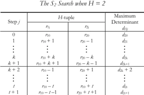
TABLE 3.1 The S2 Search when H = 2
H-tuple Step j
r1j r2j
Maximum Determinant
dHj
0 1
#
k k + 1
r10
r10 + 1 #
r10 + k
r10 + k + 1
r20
r20 – 1 #
r20 – k
r20 – k – 1
d20
d21 #
d2k
d2k+1
k + 2
#
t t + 1
r10 – 1 #
r10 – t
r10 – t –1
r20 + 1 #
r10 + t
r20 + t +1
d2k + 2 #
d2t
d2t+1
The above table is set up as follows:
i. Start at j = 0 with guessed values of r10 and r20; r10 + r20 = N; r10, r20
≥
0.ii. Arrange the n10 n20 available designs at j = 0 into n20 sets, each set containing
n10 designs that satisfy theorem 1.
iii. Apply theorem 2 to compare the designs and so obtain the best determinant value in each set and let these be d1, d2, ..., dn20,
iv. Set d20 = max{di}; i = 1, 2, ..., n20
v. Repeat (i) – (iv) at j = 1, 2, ..., t+1 and thus obtain d2k and d2t;
d21 < d22 < ... < d2k > d2k + 1; d2k+ 2 < d2k + 3 < ... <d2t > d2t + 1.
vi. Set d2* = max{d20, d2k, d2t} and the corresponding design ξN* as the
D-optimal design.
S3 Search for H = 3
1. Begin at j = 0 with guessed values of a 3-tuple (r10, r20, r30); where r10, r20, r30
are respectively the number of support points from balls 1, 2, 3 and N = r10
+ r20 + r30; r10, r20, r30
≥
0.2. Holding, for example, r10 fixed, perform the S2 (H = 2) search at j = 0
be-tween balls 2 and 3 to obtain the maximum determinant value d30(1), showing
that this value is obtained at fixed value (r10) of ball 1.
3. Repeat the S2 search at other values of r10; namely, r10 + 1, r10 + 2, ..., r10 + k
+1, r10 – 1, r10 – 2, ..., r10 – t – 1. Hence, obtain d3k(1) and d3t(1).
4. Define d3* = max{d30(1), d3k(1), d3t(1)} to be the global value of the determinant
of the information matrices and the corresponding ξN* as the D-optimal de-sign.
General case of SH search
1. Begin at j = 0 with guessed values of the H-tuple, ( , , r10 r20 ..., );rH0
i0 i0 =1
= H , 0 i
N
∑
r r ≥ .2. The first H – 2 values, i.e. r10, ..., rH – 2,0 are held fixed and an S2 search is
per-formed on balls H – 1 and H to obtain dH0(1, 2, ..., H – 2).
3. An S3 search is now performed on the last three balls; namely, H – 2, H – 1,
and H to obtain dH0(1, 2, ..., H – 3).
4. In a similar way an S4 search, gives a dH0(1, 2, ..., H – 4) and so on to SH that yields
dH0.
5. Set dH0= max{dH0(1, ..., H -2), ..., dH0(1)}.
6. Finally, searching at other values of r10; namely at r10 + 1, r10 + 2, ..., r10 + k,
r10+ k + 1, r10 – 1, r10 – 2, ..., r10 – t, r10 – t – 1,we obtain dHk and dHt.
7. Set dH* = max{dH0, dHk, dHt} and the corresponding ξN* as the D-optimal ex-act design.
As stated in section 2, theorems 1 and 2 have the effect of reducing the num-ber of determinantal calculations and thus speeding up the rate of convergence of the algorithm. Further increases in the rate of convergence come as a result of the occurrence of singular designs as well as the fact that some rij’s quickly become zero.
Theorem 3. The sequence S2, S3, ..., SH is convergent to the global D-optimal exact
design.
Proof: Since the sequence S3, ..., SH require progressive repeat of S2, it is sufficient
to prove that S2 is convergent. The concavity of det(M(ξN)); see, e.g. Pazman
(1986), means that d2k and d2t are respectively the only local maxima in the
in-creasing and dein-creasing directions of he search. Therefore, * 2
d is a global opti-mum.
4. A NUMERICAL EXAMPLE
We consider an application of the algorithm to obtain a D-optimal 6-point de-sign for a bivariate quadratic surface defined on the unit cube i.e.
2 2
1 2 00 10 1 20 2 12 1 2 11 1 22 2
( , ) = + + + + + +
f x x a a x a x a x x a x a x e;
2
1 2 1 2
= { , ; , = -1, 0, 1}, e = 1
The three balls 1 = 1 1 1 1 , = 2 1 0 1 0 , = 3 0
1 1 1 1 0 1 0 1 0
g ⎛⎜− − ⎞⎟ g ⎛⎜− ⎞⎟ g ⎛ ⎞⎜ ⎟
− − −
⎝ ⎠ ⎝ ⎠ ⎝ ⎠
are of sizes n1 = n2 = 4, n3 = 1. The combinatorics for this case of H = 3 are
given in the table hereunder:
TABLE 4.1
An S3 search for 6-point D-optimal design for a quadratic surface defined on a cubic space
Step j r 3-tuple
1j r2j r3j
Maximum determinant dHj
Number of
designs at step j D-optimal designs Number of
0
1
2
3
4
3 3 0
4 2 0
5 1 0
2 4 0
1 5 0
1.3717 × 10⁻³
5.4870 × 10⁻³
singular
1.3717 × 10⁻³
singular
16
6
16
6
16
4
5
6
7
8
9
3 2 1
4 1 1
5 0 1
2 3 1
1 4 1
3.0864 × 10⁻³
5.4870 × 10⁻³
singular
3.4214 × 10⁻⁴
3.4214 × 10⁻⁴
24
4
4
24
4
all 4
At j = 0, for example, the sixteen designs are:
( )1 ( )2 ( )4 ( )5 ( )16
6 = 0, 6 = 0, ..., 6 = 0; 6 = 0, ..., 6 = 0
0 0 0 0 0
0 0 0
ξ ξ ξ ξ ξ
− − − − + − − − − +
+ − − + − + + − + −
− + + + + + − + + +
− − − − −
− − − − +
+ − + − + + +
The first set of four designs have the corresponding diagonal elements of their information matrices equal, then the next set of four, etc. Now applying theorem 2 on the off-diagonal elements for designs within a set, one can establish the fol-lowing equalities (inequalities): (M3 = M1) < (M2 = M4); (M7 = M5) < (M6 = M8);
(M11 = M12) < (M9 = M10); (M15 = M16) < (M13 = M14). Comparing between sets,
we see that M2 = M9 and M6 = M14.
( )4 ( )11 ( )14 ( )21
6 6 6 6
6 0 0 1 4 4
0 4 1 1 0 1
0 1 4 1 1 0
( ) ( ) ( ) ( ) .
1 1 1 3 1 1
4 0 1 1 4 3
4 1 0 1 3 4
M ξ M ξ M ξ M ξ
−
⎛ ⎞
⎜ − ⎟
⎜ ⎟
⎜ − ⎟
= = = = ⎜− − − ⎟
⎜ ⎟
⎜ − ⎟
⎜ ⎟
⎜ − ⎟
⎝ ⎠
The rest are either inferior designs, based on theorem 2, or they are singular de-signs.
On combinatorial and variance exchange methods
Using the combinatorial technique, it is easy to determine all the designs that are concurrently D-optimal. The experimenter can therefore choose one of these designs on the basis of convenience and minimality of cost.
The variance exchange method works well for approximate designs; i.e. when the equivalence between the G- and D-optimality applies. But for exact designs the method can fail because the equivalence of the G- and D-optimality criteria no longer applies. On the other hand, the combinatorial technique can be applied to both exact and approximate designs.
The phenomenon of cycling which often occurs in a variance exchange tech-nique; see, Atkinson and Donev (1992), cannot occur in the method of combina-torics.
Department of Statistics IKEBASILONUKOGU
University of Nigeria, Nsukka Enugu State, Nigeria
Department of Mathematics/Statistics MARYPASCALIWUNDU
University of Port-Harcourt Rivers State, Nigeria
REFERENCES
A. C. ATKINSON, A. N. DONEV, (1992), Optimal Experimental Design, Oxford University Press. G. E. P. BOX, N. R.DRAPER, (1959), A basis for the selection of a response surface design, “Journal of
American Statistical Association”, vol. 54, pp. 622-654.
N.R. DRAPPER, J.A. JOHN,(1998), Response Surface Designs Where Levels of Some Factors are Difficult to Change, “Australian and New Zealand Journal of Statistics”, vol. 40, no. 4, pp. 487-495.
V.V. FEDOROV,(1972), Theory of Optimal Experiment. Academic Press, New York.
T. J MITCHELL, (1974), An Algorithm for the Construction of D-Optimal Experimental Designs,
“Technometrics”,16,203-210.
T. J. MITCHELL,(2000), An Algorithm for the Construction of “D-Optimal” Experimental Designs,
I B. ONUKOGU, (1997), Foundations of Optimal Exploration of Response Surfaces, Ephrata Press,
Nsukka, Nigeria.
I.B. ONUKOGU, P.E CHIGBU, (2002),Super Convergent Line Series in Optimal Design of Experiments and Mathematical Programming, AP Express Publishers, Nsukka, Nigeria.
A. PAZMAN,(1986), Foundations of Optimum Experimental Designs, D. Riedel Publishing
Com-pany.
A. I. STREET, D.J STREET,(1987), Combinatorics of Experimental Design, Oxford University Press.
SUMMARY
A combinatorial procedure for constructing D-optimal exact designs
The basic problem considered in this paper may be stated as follows: find an N-point exact design measure ξN which maximizes the determinant of the information matrix of
a given response function f(x), where x is an n-component vector of non-stochastic vari-ables defined in a space of trial X .