DISTRIBUTIONS OF PRODUCTS INVOLVING THE TYPE II BESSEL FUNCTION RANDOM VARIABLE
M. Garg, J. Agrawal, S. Nadarajah
1. INTRODUCTION
The distribution of product of independent random variables (r.v.s) is of inter-est in many areas of science and econometrics. The distribution of product of in-dependent r.v.s X and Y has been studied by several authors especially when X and Y belong to the same family of distributions. In this context the names of Sakamoto (1943), Stuart (1962), Springer and Thompson (1970), Podolski (1972), Steece (1976), Wallgren (1980), Bhargava and Khatri (1981), Abu-Salih (1983), Tang and Gupta (1984), Malik and Trudel (1986) and most recently those of Gli-ckman and Xu (2008)are of great importance.
In the present paper we shall study the distribution of XY as well as of |XY| when X and Y are independent r.v.s belonging to different families of tions. Here we assume that the r.v. X follows the type II Bessel function distribu-tion given as follows
Type II Bessel function distribution (Springer, 1979)
-12
( ) | | exp - ( | |)
2
x
f x D x I x
; x ( , ) (1)
2
2 -1 -( / )
; 0, 0, 0
2
e where D
(2)
2 0
1 and ( )
! ( 1) 2
m
m
x I x
m m
(3)
( ) is the modified Bessel function of the first kind.
This distribution generalizes the well known Rayleigh distribution, Chi distribu-tion, noncentral Chi distribution and folded normal distribution (Springer, 1979).
Normal distribution
2 2
( )
1
( ) exp
-2 2
y
g y
; y ( , ), >0 (4)
Pearson VII distribution
1-2 2 1
2
( ) 1 ; ( , ), 1, 0
( 1)
M
M y
g y y M N
N
N M
(5)
Maxwell Boltzmann distribution (Mathai, 1993) 3
2 2
2 2
( ) exp( ) ; 0, ( , )
g y y y y
(6)
We shall require the following definitions in the sequel
Modified Bessel function of the third kind (Gradshteyn and Rhyzik, 1994) 1
2 2
1
( ) ( 1) exp( )
1 2
2
x
K x t xt dt
, + ½ >0 (7)
Tricomi’s function(Srivastava and Manocha, 1984)
1 1
0 1
( , ; ) (1 ) ,
( )
b a zt a
a b z e t t dt
a
a > 0, z > 0 (8)
(1 )
1 1 1 1
(1 ) ( 1)
( , ; ) ( ; ; ) ( 1; 2 ; )
( 1) ( )
b
b b
a b z F a b z z F a b b z
a b a
(9)
Kampé de Feriét function (Srivastava and Manocha, 1984)
1 1 1
: ;
: ; , 0
1 1 1
( ) ( ) ( )
( ):( ) ;( ); ,
( ):( );( ); ( ) ( ) ( ) ! !
p q k
s r
j r s j r j s
j j j
p q k
p q k
l m n
l m n r s
l m n j r s j r j s
j j j
a b c
a b c x y
F x y
r s
,
(10)
(i) p + q < l + m + 1, p + k < l + n + 1, |x| < , |y| < , or (11) (ii) p + q = l + m + 1, p + k = l + n +1, and
1/( ) 1/( )
1, ,
max{ , } 1,
p l p l
x y if p l
x y if p l
(12)
2. THE DISTRIBUTION OF THE PRODUCT OF TWO INDEPENDENT RANDOM VARIABLES THAT ARE NOT EVERYWHERE POSITIVE
Let a r.v. X has the probability density function (p.d.f.) f(x), which can be writ-ten as
f(x) = f –(x) + f +(x) , - < x < (13)
in which f –(x) vanishes identically except on the interval - < x < 0 , where f –(x) = f(x).
Similarly f +(x) is defined to be identically zero except over the interval 0 x <
, where f +(x) = f(x).
Let X and Y be two independent r.v.s with p.d.f. f(x) and g(y), respectively. We know that the p.d.f. h(z) of the r.v. Z=XY is given by (Springer, 1979)
h(z) =
-
-1 f x g( ) z dx 1 f z g y dy( )
x x y y
(14)Using the concept of partitioning as given by (13) for both f(x) and g(y), the a-bove expression can be written as
-
--
-1 1
( ) ( ) ( )
1 1
( ) ( )
z z
h z f x g dx f x g dx
x x x x
z z
f x g dx f x g dx
x x x x
(15)
We shall write h(z) as
h(z) = h–(z) + h+(z) , - < z < (16)
in which
( ) , 0
( )
0 , 0
h z z
h z
z
(17)
0 , 0 ( )
( ) , 0
z h z
h z z
(18)
In the special case, when f(x) and g(y) are even functions i.e. f+(x) = f–(-x) and g+(y) = g-(-y), eq. (15) can be simplified as follows. For z 0,
0 0
0 0
0
1 1
( ) ( ) 0 ( ) ( ) 0
1 1
( ) ( )
1
2 ( ) .
z z
h z h z f x g dx f x g dx
x x x x
z z
f x g dx f x g dx
x x x x
z
f x g dx
x x
(19)
For 0 z ,
0 0
0 0
0
1 1
( ) ( ) ( ) 0 0 ( )
1 1
( ) ( )
1
2 ( ) .
z z
h z h z f x g dx f x g dx
x x x x
z z
f x g dx f x g dx
x x x x
z
f x g dx
x x
(20)
Thus in this case when f(x) and g(y) are even functions, we have
0 1
2 ( ) ; 0
( )
0 ; 0
z
f x g dx z
h z x x
z
(21)and
0
0 ; 0
( ) 2 1 ( ) ; 0
z
h z z
f x g dx z
x x
(22)
2
1
2 2 4 ( /2 ) 4 2 2
1
2 2 2 2
0 2 2 1 ( ) ! ( ) 2 16 k k k z z
h z e K z
k k z
– < z < (23)
where > 0, θ > 0, λ > 0, > 0, λ - (1/2) 0, 1, 2,... and Kv(.) is given by (7). The cumulative density function (c.d.f.) H(z) of z is given by
2 2
( /2 )
2 2
1 1
1 1 2 1 2
( ) 1( ) ( )
2 2 ( ) 2 3 ( )
z
H z e A z z A z
(24) where
2 2 2
1:1;0
2:2;0 2 2
1
; 1; -;
( ) 1 1 - ,
, ; , ; -; 8 4
2 2
z z
A z F
, (25)
2 2 2 2 0 0 1 1 2 4 2 2 ( )3 ! !
( ) 2
r k
k r r
k r k r z A z k r
(26)
where F(.) is given by (10).
Proof : Since the p.d.f.s f(x) and g(y) as given by equations (1) and (4) are even, we shall use the results (21) and (22) to calculate the value of h(z). Substituting the values of f(x) and g(- z/x) from equations (1) and (4) in eq.(21) we get
2 2
-( /2 ) 2
1
1
-1 2
0
1 1
( ) exp - ( )exp
2 2
2
z
e x
h z x I x dx
x
, (27)-< z < 0
Next, writing the modified Bessel function Iv(x) in its series form (3) and us-ing the followus-ing known integral (Gradshteyn and Rhyzik, 1994)
2 1
0
2
exp( p p) p (2 ( )) Re 0, Re 0
p
x x x dx K
1
2 4
2
2 4 2 2
-( /2 )
1
2 2 2 2
2 0
2 1
( ) ( )
! ( )
2 16
k
k k
z z
h z e K z
k k
z
(29)
- < z < 0
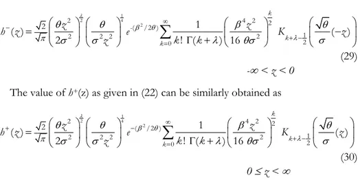
The value of h+(z) as given in (22) can be similarly obtained as
1
2 4
2
2 4 2 2
( /2 )
1
2 2 2 2
2 0
2 1
( ) ( )
! ( )
2 16
k
k k
z z
h z e K z
k k
z
(30)
0 z <
Now using the equation (16) and combining the results (29) and (30), we get the required p.d.f. h(z) as given by equation (23).
The c.d.f. of z is defined as
H(z) =
0
0 0
1
( ) ( ) ( ) ( )
2
Z Z Z
h z dz h z dz h z dz h z dz
(31)[since the p.d.f. f(x) and g(y) are even, h(z) is also an even function and
( ) 1
h z dz
]Writing the value of h(z) from eq. (23), using the known result (Prudnikov, Brychov and Marichev, 1986) as mentioned below
2 1
- 1 1 2 0
2 1
1 1 2
2 ( ) 1 3
( ) ;1 , ;
4
( 1) 2 2
2 ( ) 1 3
;1 , ;
4
( 1) 2 2
x x
K x dx x F
x
x F
(32) ( ReRe 1)
and applying some useful properties of hypergeometric functions, we get the re-quired result (24).
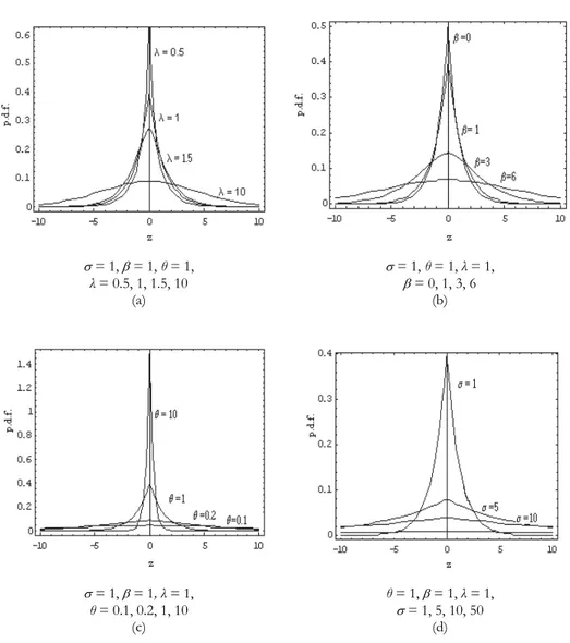
Fig. 1illustrates possible shapes of the p.d.f. (23) for (a) = 1, = 1, θ = 1 and λ
= 1, = 1, θ = 1, = 1, θ = 1, λ = 1,
λ = 0.5, 1, 1.5, 10 = 0, 1, 3, 6
(a) (b)
= 1, = 1, λ = 1, θ = 1, = 1, λ = 1,
θ = 0.1, 0.2, 1, 10 = 1, 5, 10, 50
(c) (d)
Fig. 1 – Different possible shapes of the p.d.f. (23) for specified values of parameters λ, , θ and . Corollary 1 If X and Y are independent r.v.s as given in Theorem 1, then the p.d.f.
h(w) and c.d.f. H(w) of W = |XY| are given by
1
2 4
2 2 4 2 2
( /2 )
1
2 2 2 2
2 0
2 2 1
( )
! ( )
2 16
k
k k
w w
h w e K w
k k
w
(33)
2
2( /2 )
1 2
2
1 1
1
1 2 2
( ) ( )- ( )
( ) 2 3 ( )
w
H w e A w w A w
(34)
0 w <
where > 0, θ > 0, λ > 0 ,
0 and A1(w) and A2(w) are given by eq. (26).Proof: The result (33) for the p.d.f. of w is a direct consequence of (23) and the relation
h(w) = 2 h(z) ; 0 z < (35)
and the result (34) for the c.d.f. of w follows from the relation H(w) = 2 H(z);0 z < where H(z) is given by (24). ■
Corollary 2 Let the r.v X follow the Rayleigh distribution (Springer, 1979) defined as follows
2( ) | |exp 2 ; 0, ( , )
2
x
f x x x (36)
and the independent r.v Y follow the normal distribution defined by (4), then the p.d.f. h(z) and the c.d.f. H(z) of Z = XY are given by
1 3 2 4
1 6
2 2
( )
4
z
h z K z
(37)
and
2 2 2
1
0 1 2 2 2 1 2 3 2
1 1 1
( ) ; ; 1; , 2;
2 2 4 4 2 4
z z z
H z z F F
- < z < (38)
where > 0, θ > 0
Proof: On taking = 0 and λ = 1 in Theorem 1, the type II Bessel function distri-bution reduces to the Rayleigh distridistri-bution and we easily arrive at the above re-sult. ■
Remark 1 Note that the p.d.f.s given by Theorem 1 and Corollary 1 are infinite
Theorem 2 Let X be a r.v. following the type II Bessel function distribution given by (1) and Y be an independent r.v. following the Pearson VII distribution given by (5), then the p.d.f h(z) of Z=XY is given by
22
( /2 )
2 2 2 1:0;0
1:1;0 1
2 2 2 2
4 1
( )
2
1 ( 1) 1 ; -; -;
2 ,
1; ; -;
( ) ( 1) 2 4 2
1 1
2 2 1 1
2, 2, ; ,
2 ( 1) ( ) 2 2
z
h z e
N z
M
M z z
F
M N N
M
z z
H M
N M N
- < z < (39)
where θ, λ, N > 0, M > 1,
0, 2 2
< 1 , λ-(1/2) 0,
1, 2,...
F(.) is given by (10) and H4(.) (Erdelyi, 1953) is defined as follows
4 , 0 ( ) ( ) ( , , , , ) ( ) ! ! m n m n n
m n m
a
H x y x x
m n
(40)Also the c.d.f of Z is given by
2
( /2 ) 1
1 2
2
1 ( 1) ( )
2 ( )
1 1 2 ( 1)
( )
2 2 ( 1) ( )
1 1 ( )
2 2 2
M
B z e
H z
N M
z M B z
N (41) where
2 2 2
2:0;0
1 2:1;0 1
2
1 , ; -; -;
( ) 1 ,
, 2; ; -; 4 2
M z z
B z F
N N (42)
2 2 2 0 01 1 1
2 2
2 2 2
( )
3 ! !
( ) 2
r k
k r r r
k r k
r z M N B z k r
(43)Proof: Substituting the values of f(x) and g(- z/x) from equations (1) and (5) in eq.(21), we obtain
2
1 2 2 ( /2 )
1 1 1 0 ( ) 1 2
2 exp - ( ) 1
2 ( 1) M h z z M
e x x I x x dx
N N M
(44)Writing the modified Bessel function in series form (3) and using the following known integral (Gradshteyn and Rhyzik, 1994)
1 0
(1 ) ( ) ( , 1 ) [ Re 0, Re 0, Re 0]
px q q
e x ax dx a q q q q p a
(45) we get
2 2-( /2 )
2 2 2
0
( )
1 2 ( )
( 1) 2
( 1) 1
1; 2;
! ( ) 4 2
1
k k z M z h z M Nk M z z
k M k
k k N N
e
(46) where (a, b, z) is given by (8).Writing the Tricomi’s function (, , z) in terms of 1F1(a, b, z) as given by (9), and simplifying the result using some properties of hypergeometric functions, we obtain
2 1 2 2( /2 )
2 2 2
1:0;0 1:1;0
2 2 2
4
(-z)
z (z)
2
1 ( 1) 1 ; -; -;
z z
2 ,
1 ; ; -;
( ) ( 1) 2 4 2
1 1
z 2 2 1 1 z
2, 2, ; ,
2 ( 1) ( ) 2 2
1 h e N M M F
M N N
M
H M
N M N
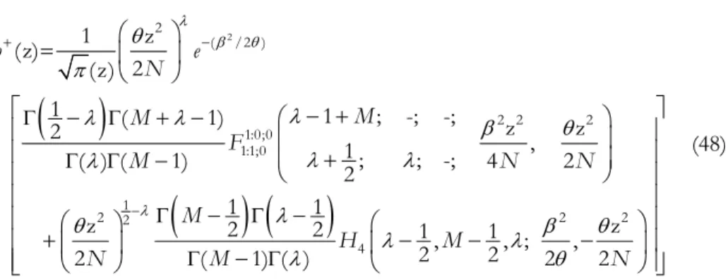
Similarly, h+(z) as given by (22) can be obtained as
2
2
( /2 )
2 2 2
1:0;0 1:1;0 1
2 2 2 2
4
1 z
(z)
2 (z)
1 ( 1) 1 ; -; -;
z z
2 ,
1 ; ; -;
( ) ( 1) 2 4 2
1 1
z 2 2 1 1 z
, , ; ,
2 2
2 ( 1) ( ) 2 2
h e
N
M M
F
M N N
M
H M
N M N
(48)
Now using the equation (16) and combining the results (47) and (48) we get the required p.d.f. h(z) as given by eq. (39). The c.d.f. of z can easily be obtained on using the result (39) in (31) which after simplification yields the required result (41). ■
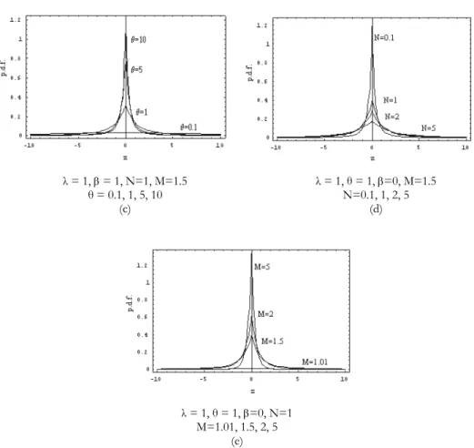
Fig. 2illustrates possible shapes of the p.d.f. (39) for (a) N=1, M=1.5, = 1, θ= 1 and λ= 0.01, 0.1, 1, 10, (b) N=1, M=1.5, θ= 1, λ = 1 and = 0.01, 0.1, 1, 5, (c) N=1, M=1.5, = 1, λ = 1 and θ = 0.1, 1, 5, 10, (d) θ = 1, = 0, λ = 1, M=1.5 and N=0.1, 1, 2, 5 and (e) θ = 1, = 0, λ= 1, N=1 and M=1.01, 1.5, 2, 5. The effect of the parameters is evident.
= 1, θ = 1, N=1, M=1.5 λ = 1, θ = 1, N=1, M=1.5
λ = 0.01, 0.1, 1, 10 = 0.01, 0.1, 1, 5
λ = 1, = 1, N=1, M=1.5 λ = 1, θ = 1, =0, M=1.5
θ = 0.1, 1, 5, 10 N=0.1, 1, 2, 5
(c) (d)
λ = 1, θ = 1, =0, N=1 M=1.01, 1.5, 2, 5
(e)
Fig. 2 – Different possible shapes of the p.d.f. (39) for specified values of parameters λ, , θ, N and M.
Corollary 3 If X and Y are independent r.v.s as given in Theorem 2, then the p.d.f. h(w) and the c.d.f. H(w) of W= |XY| are given by
2 2
1 2
2
2 2 2
1:0;0
1:1;0 1 2 1
2 2 2 2
1
4 2
2
( )
2
1 ( 1)
1 ; -; -;
2 ,
; ; -;
( ) ( 1) 4 2
1
2 1
, 2, ; ,
2 ( 1) ( ) 2 2
w
h w w
N
M M w w
F
M N N
M
w H M w
N M N
e
(49)
2
-( /2 ) 1
1 2
2
1 ( 1) ( )
2 ( )
2 ( 1) ( )
2 ( 1) ( )
1 1 ( )
2 2 2
2
M
B w H w
N M
w M B w
N e (50)
0 w <
where θ, λ, N > 0 , M > 1,
0, and B1(w)and B2(w) as defined by (42) and (43) respecttively.Proof: Result (49) for the p.d.f. of w is a direct consequence of (39) and the relation
h(w) = 2 h(z) ; 0 z < (51)
and the result (50) for the c.d.f. of w follows from the relation
H(w) = 2 H(z) ; 0 z < (52)
where H(z) is given by (41). ■
Corollary 4 Let the independent r.v. X follow the type II Bessel function distribu-tion given by (1) and the r.v Y follow the student-t distribudistribu-tion (Johnson and Kotz, 1970) defined as follows
1 2 2 1 2 2 1( ) 1 ; (- , ), 0
,
y
g y y
B
(53)
then the p.d.f. h(z) and c.d.f. H(z) of Z = XY are given by
2 2
2 2 2
1 2 2 1:0;0
1:1;0
1 2 2
2
4 ( )
2
1 ; -; -;
2 2 ( ) 2 ,
4 2 1 ( ) ; ; -; 2 2 1 1
2 1 1
2 2
, , ; ,
2 ( ) 2 2 2 2 2
and
2 1 2 1 ( /2 )-2 1
2 2 ( )
2 ( 1)
1 2
( ) 2
2 2 1
2 ( )
( ) 2
1
D z H z
z D z
e
- < z < (55)
where θ > 0, > 0, λ > 0
2 2 2
2:0;0 1 2:1;0
, ; -; -; 2
( ) - , ,
1, 1; ; -; 4 2
2
z z
D z F
(56)
2 2 2 0 01 1 1
2 2
2 2 2 2
( )
3 ! !
( ) 2
r k
k r r r
k r k
r z D z k r
(57)Proof: If N = and M = 1 + /2 the Pearson VII distribution reduces to the stu-dent-t distribution, thus the above results can easily be obtained by setting N =
and M = 1 + /2 in Theorem 2. ■
Theorem 3 Let X be a r.v. following the type II Bessel function distribution given by (1) and Y be an independent r.v. following the Maxwell-Boltzmann distribu-tion given by (6), then the p.d.f h(z) of Z=XY is given by
1 4 2
3 2
2 4 2 ( 2/2 ) 2 4
3 2 0
4 1
( ) ( ) ( 2 )
2 ! ( ) 8
k
k k
e z
h z z K z
k k
(58) and
2 32 2 2
( /2 )
1 2
3 3
1 1 2 2
( ) ( ) ( )
2 ( 1) 2 ( ) 2
z z
H z e C z C z
(59)
where θ, λ, > 0,
0, k + λ - (1/2) 0, 1, 2,... and2 2
1:0;0
1 2:1;0 1
2
; -; -;
( ) - , ,
1, ; ; -; 4 2
z z
C z F
(60)
2 2
2
0 0
3 3
2 2
2 2
( )
5 ! !
( ) 2
r k
k r r
k r k
r
z
C z
k r
(61)Proof: Substituting the values of f(x) and g(- z/x) from equations (1) and (6) in eq. (21) as follows
2 2 2
3 ( /2 ) 2
1 2
1 1
0
2
( ) e exp x2 ( ) z exp z
h z x I x dx
x x
(62)
- < z < 0
Next, writing the modified Bessel function in series form and using the known result (Gradshteyn and Rhyzik, 1994) given in Theorem 1, we get h-(z) as follows
3 4 2
1 2
2 4 2 ( 2/2 )
2 4
3 2 0
4 1
( ) ( ) ( 2 ( ))
2 ! ( ) 8
k k k
e z
h z z K z
k k
(63)
- < z < 0
Similarly, h+(z) can be obtained as
2
3 4 2
1 2
2 4 2 ( /2 ) 2 4
3 2 0
4 1
( ) ( ) ( 2 )
2 ! ( ) 8
k
k k
e z
h z z K z
k k
(64)
0 z <
Now using the equation (16) and combining the results (63) and (64) we can get the required p.d.f. as given by eq. (58).
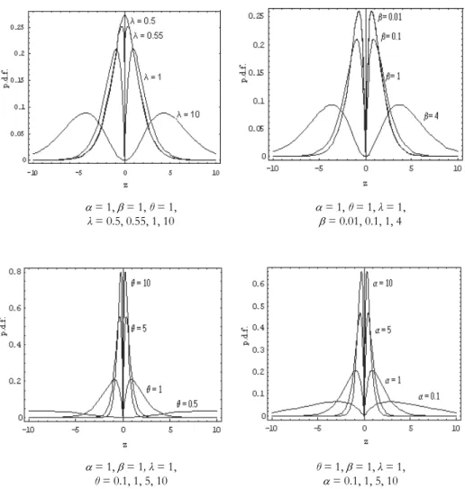
Fig. 3 illustrates possible shapes of the p.d.f. (58) for (a) = 1, = 1, θ = 1 and
λ = 0.5, 0.55, 1, 10, (b) = 1, θ = 1, λ = 1 and = 0.01, 0.1, 1, 4, (c) = 1, = 1,
λ = 1 and θ = 0.1, 1, 5, 10 and (d) θ = 1, = 1, λ= 1 and = 0.1, 1, 5, 10. The effect of the parameters is evident
= 1, = 1, θ= 1, = 1, θ= 1, λ= 1,
λ= 0.5, 0.55, 1, 10 = 0.01, 0.1, 1, 4
= 1, = 1, λ = 1, θ= 1, = 1, λ = 1,
θ= 0.1, 1, 5, 10 = 0.1, 1, 5, 10
Fig. 3 – Different possible shapes of the p.d.f. (58) for specified values of parameters λ, , θ and . Corollary 5 If X and Y are independent r.v.s as given in Theorem 3, then the p.d.f h(w) and the c.d.f H(w) of W= |XY| are given by
2
1 4 2
3 2
2 4 2 ( /2 ) 2 4
3 2 0
8 1
( ) ( ) ( 2 )
2 ! ( ) 8
k
k k
e w
h w w K w
k k
and
32 2 2
2 -( /2 )
1 2
3 3
2 2 2
( ) ( ) ( )
( 1) 2 ( ) 2
w w
H w e C w C w
(66)
0 w <
where θ, λ, > 0
0 and C1(w) and C2(w) as defined by (60) and (61) respectively.Proof: Result (65) for the p.d.f. of W is a direct consequence of (58) and the rela-tion
h(w) = 2 h(z) ; 0 z < (67)
and the result (66) for the c.d.f. of W follows from the relation
H(w) = 2 H(z) ; 0 z < (68)
where H(z) is given by (59). ■
Corollary 6 Let the independent r.v. X follow the Chi distribution (Springer, 1979) given as follows
22 1
2 2
1
( ) | | exp ; ( , ), 0, 0
( ) 2 2
x
f x x x
(69)
and the independent r.v Y follow the Maxwell-Boltzmann distribution given by (6), then the p.d.f. h(z) and the c.d.f. H(z) of Z = XY are given by
1
1 2 4
2 2 4
3
2
-2
4 1 2
( ) ( )
( ) 2
h z z K z
, - < z < , (70)
and
2 2
1 2
2 2
3
2 2 2
1 2
2 2
3
z z
2 ; 1, 1;
2
( 1) 2 2
1 1
(z)
2 3
z z
2 3 5 5; , ;
2 2 2
( ) 2 2
F H
F
Proof: On taking = 0 and θ= θ1/2 , λ = θ1 and replacing θ1 by θ in Theorem 3,
the type II Bessel function distribution reduces to the Chi distribution and we easily arrive at the above result. ■
Remark 2 Note that the p.d.f.s given by Theorem 3 and Corollary 5 are infinite
mixtures of type I Bessel function distributions. The p.d.f. given by Corollary 6 is precisely that of a type I Bessel function distribution.
ACKNOWLEDGEMENTS
The authors would like to thank the Editor and the referee for carefully reading the paper and for their comments which greatly improved the paper.
Department of Mathematics MRIDULA GARG
University of Rajasthan Jaipur 302004 India
E-mail: [email protected]
Department of Mathematics JAYA AGRAWAL
University of Rajasthan Jaipur 302004 India
E-mail: [email protected]
School of Mathematics SARALEES NADARAJAH
University of Manchester Manchester M13 9PL UK
E-mail: [email protected]
REFERENCES
M. S. ABU-SALIH, (1983), Distribution of the product and the quotient of power-function random
vari-ables, “Arab Journal of Mathematics”, 4, pp. 77-90.
R. P. BHARGAVA, C. G. KHATRI, (1981), The distribution of product of independent beta random variables
with application to multivariate analysis, “Annals of the Institute of Statistical Mathematics”, 33, pp. 281-287.
A. ERDÉLYI, et al. (eds), (1953), Higher Transcendental Functions, Volume I, McGraw-Hill, New
York.
T. S. GLICKMAN, F. XU, (2008), The distribution of the product of two triangular random variables,
“Statistics and Probability Letters”, in press.
I. S. GRADSHTEYN, I. M. RHYZIK, (1994), Table of Integrals, Series, and Products, fifth edition,
Aca-demic Press, San Diego.
N. L. JOHNSON, S. KOTZ, (1970), Continuous Univariate Distributions , Volume 2, John Wiley and
Sons, New York.
H. J. MALIK, R. TRUDEL, (1986), Probability density function of the product and quotient of two correlated
A. M. MATHAI, (1993), A Handbook of Generalized Special Functions for Statistical and Physical
Sci-ences, Clarendon Press, Oxford.
H. PODOLSKI, (1972), The distribution of a product of n independent random variables with generalized
gamma distribution, “Demonstratio Mathematica”, 4, pp. 119-123.
A. P. PRUDNIKOV, Y. A. BRYCHOV, O. I. MARICHEV, (1986), Integrals and Series Volumes I and II,
Gordon and Breach Science Publishers, Amsterdam.
H. SAKAMOTO, (1943), On the distribution of the product and the quotient of the independent and
uni-formly distributed random variables, “Tohoku Mathematical Journal”, 49, pp. 243-260.
M. D. SPRINGER, (1979), The Algebra of Random Variables, John Wiley and Sons, New York. M. D. SPRINGER, W. F. THOMPSON, (1970), The distribution of products of beta, gamma and Gaussian
random variables, “SIAM Journal on Applied Mathematics”, 18, pp. 721-737.
H. M. SRIVASTAVA, H. L. MANOCHA, (1984), A Treatise on Generating Functions, John Wiley and
Sons, New York.
B. M. STEECE, (1976), On the exact distribution for the product of two beta-distributed random variables,
“Metron”, 34, pp. 187-190.
A. STUART, (1962), Gamma-distributed products of independent random variables, “Biometrika”, 49,
pp. 564-565.
J. TANG, A. K. GUPTA, (1984), On the distribution of the products of independent beta random variables,
“Statistics and Probability Letters”, 2, pp. 165-168.
C. M. WALLGREN, (1980), The distribution of the product of two correlated t variates, “Journal of the
American Statistical Association”, 75, pp. 996-1000.
SUMMARY
Distributions of products involving the type II Bessel function random variable