The PLAN Procedure (Chapter)

(1)

SAS/STAT

®

9.3 User’s Guide

The PLAN Procedure

(Chapter)

(2)

Cary, NC: SAS Institute Inc.

For a Web download or e-book: Your use of this publication shall be governed by the terms established by the vendor at the time you acquire this publication.

The scanning, uploading, and distribution of this book via the Internet or any other means without the permission of the publisher is illegal and punishable by law. Please purchase only authorized electronic editions and do not participate in or encourage electronic piracy of copyrighted materials. Your support of others’ rights is appreciated.

U.S. Government Restricted Rights Notice: Use, duplication, or disclosure of this software and related documentation by the U.S. government is subject to the Agreement with SAS Institute and the restrictions set forth in FAR 52.227-19, Commercial Computer Software-Restricted Rights (June 1987).

SAS Institute Inc., SAS Campus Drive, Cary, North Carolina 27513. 1st electronic book, July 2011

SAS®Publishing provides a complete selection of books and electronic products to help customers use SAS software to its fullest potential. For more information about our e-books, e-learning products, CDs, and hard-copy books, visit the SAS Publishing Web site atsupport.sas.com/publishingor call 1-800-727-3228.

SAS®and all other SAS Institute Inc. product or service names are registered trademarks or trademarks of SAS Institute Inc. in the USA and other countries. ® indicates USA registration.

(3)

Chapter 67 The PLAN Procedure

Contents

Overview: PLAN Procedure . . . 5585

Getting Started: PLAN Procedure . . . 5587

Three Replications with Four Factors . . . 5587

Randomly Assigning Subjects to Treatments . . . 5588

Syntax: PLAN Procedure. . . 5590

PROC PLAN Statement . . . 5590

FACTORS Statement . . . 5590

OUTPUT Statement . . . 5593

TREATMENTS Statement. . . 5595

Details: PLAN Procedure. . . 5596

Using PROC PLAN Interactively . . . 5596

Output Data Sets . . . 5597

Specifying Factor Structures . . . 5599

Randomizing Designs . . . 5601

Displayed Output. . . 5601

ODS Table Names . . . 5602

Examples: PLAN Procedure . . . 5602

Example 67.1: A Split-Plot Design . . . 5602

Example 67.2: A Hierarchical Design. . . 5603

Example 67.3: An Incomplete Block Design . . . 5604

Example 67.4: A Latin Square Design . . . 5606

Example 67.5: A Generalized Cyclic Incomplete Block Design . . . 5607

Example 67.6: Permutations and Combinations . . . 5608

Example 67.7: Crossover Designs. . . 5612

References . . . 5616

Overview: PLAN Procedure

The PLAN procedure constructs designs and randomizes plans for factorial experiments, especially nested and crossed experiments and randomized block designs. PROC PLAN can also be used for generating lists of permutations and combinations of numbers. The PLAN procedure can construct the following types of experimental designs:

(4)

full factorial designs, with and without randomization

certain balanced and partially balanced incomplete block designs

generalized cyclic incomplete block designs

Latin square designs

For other kinds of experimental designs, especially fractional factorial, response surface, and orthogonal array designs, see the FACTEX and OPTEX procedures and the ADX Interface in SAS/QC software. PROC PLAN generates designs by first generating a selection of the levels for the first factor. Then, for the second factor, PROC PLAN generates a selection of its levels for each level of the first factor. In general, for a given factor, the PLAN procedure generates a selection of its levels for all combinations of levels for the factors that precede it.

The selection can be done in five different ways:

randomized selection, for which the levels are returned in a random order

ordered selection, for which the levels are returned in a standard order every time a selection is gen-erated

cyclic selection, for which the levels returned are computed by cyclically permuting the levels of the previous selection

permuted selection, for which the levels are a permutation of the integers1; : : : ; n

combination selection, for which themlevels are selected as a combination of the integers1; : : : ; n

takenmat a time

The randomized selection method can be used to generate randomized plans. Also, by appropriate use of cyclic selection, any of the designs in the very wide class of generalized cyclic block designs (Jarrett and Hall 1978) can be generated.

There is no limit to the depth to which the different factors can be nested, and any number of randomized plans can be generated.

You can also declare a list of factors to be selected simultaneously with the lowest (that is, the most nested) factor. The levels of the factors in this list can be seen as constituting the treatment to be applied to the cells of the design. For this reason, factors in this list are calledtreatments. With this list, you can generate and randomize plans in one run of PROC PLAN.

(5)

Three Replications with Four Factors F 5587

Getting Started: PLAN Procedure

Three Replications with Four Factors

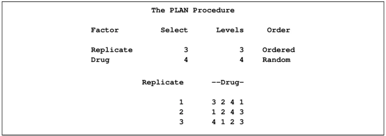
Suppose you want to determine if the order in which four drugs are given affects the response of a subject. If you have only three subjects to test, you can use the following statements to design the experiment.

proc plan seed=27371;

factors Replicate=3 ordered Drug=4; run;

These statements produce a design with three replicates of the four levels of the factorDrugarranged in random order. The three levels ofReplicateare arranged in order, as shown inFigure 67.1.

Figure 67.1 Three Replications and Four Factors

The PLAN Procedure

Factor Select Levels Order

Replicate 3 3 Ordered Drug 4 4 Random Replicate --Drug-1 3 2 4 1 2 1 2 4 3 3 4 1 2 3

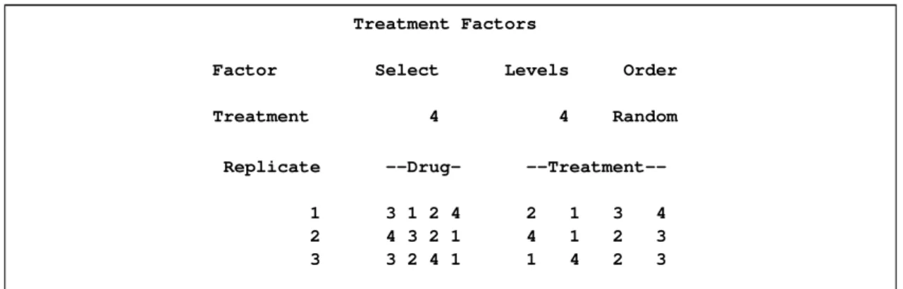
You might also want to apply one of four different treatments to each cell of this plan (for example, applying different amounts of each drug). The following additional statements create the output shown inFigure 67.2:

factors Replicate=3 ordered Drug=4; treatments Treatment=4;

run;

Figure 67.2 Using the TREATMENTS Statement

Plot Factors

Replicate 3 3 Ordered

(6)

Figure 67.2 continued

Treatment Factors

Treatment 4 4 Random

Replicate --Drug-

--Treatment--1 3 1 2 4 2 1 3 4 2 4 3 2 1 4 1 2 3 3 3 2 4 1 1 4 2 3

Randomly Assigning Subjects to Treatments

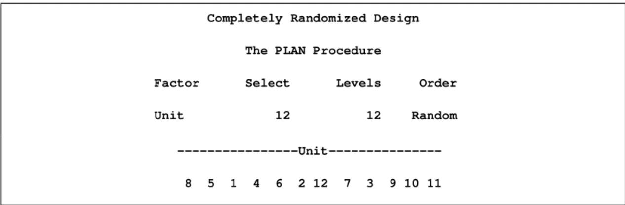
You can use the PLAN procedure to design a completely randomized design. Suppose you have 12 exper-imental units, and you want to assign one of two treatments to each unit. Use a DATA step to store the unrandomized design in a SAS data set, and then call PROC PLAN to randomize it by specifying one factor with the default type of RANDOM, having 12 levels. The following statements produce Figure 67.3and

Figure 67.4:

title 'Completely Randomized Design'; /* The unrandomized design */

data Unrandomized; do Unit=1 to 12;

if (Unit <= 6) then Treatment=1; else Treatment=2; output;

end; run;

/* Randomize the design */

proc plan seed=27371; factors Unit=12;

output data=Unrandomized out=Randomized; run;

proc sort data=Randomized; by Unit;

proc print; run;

Figure 67.3shows that the 12 levels of theunitfactor have been randomly reordered and then lists the new ordering.

(7)

Randomly Assigning Subjects to Treatments F 5589

Figure 67.3 A Completely Randomized Design for Two Treatments Completely Randomized Design

Unit 12 12 Random

---Unit---8 5 1 4 6 2 12 7 3 9 10 11

After the data set is sorted by theunitvariable, the randomized design is displayed (Figure 67.4).

Figure 67.4 A Completely Randomized Design for Two Treatments Completely Randomized Design

Obs Unit Treatment

1 1 1 2 2 1 3 3 2 4 4 1 5 5 1 6 6 1 7 7 2 8 8 1 9 9 2 10 10 2 11 11 2 12 12 2

You can also generate the plan by using aTREATMENTSstatement instead of a DATA step. The following statements generate the same plan.

proc plan seed=27371; factors Unit=12;

treatments Treatment=12 cyclic (1 1 1 1 1 1 2 2 2 2 2 2); output out=Randomized;

(8)

Syntax: PLAN Procedure

The following statements are available in PROC PLAN.

PROC PLAN<options>;

FACTORSfactor-selections</ NOPRINT>;

OUTPUTOUT=SAS-data-set<factor-value-settings>;

TREATMENTSfactor-selections;

To use PROC PLAN, you need to specify the PROC PLAN statement and at least oneFACTORS state-ment before the first RUN statestate-ment. TheTREATMENTSstatement,OUTPUTstatement, and additional

FACTORSstatements can appear either before the first RUN statement or after it.

The rest of this section gives detailed syntax information for each of the statements, beginning with the

PROC PLANstatement. The remaining statements are described in alphabetical order.

You can use PROC PLAN interactively by specifying multiple groups of statements, separated by RUN statements. For details, see the section “Using PROC PLAN Interactively” on page 5596.

PROC PLAN Statement

PROC PLAN<options>;

The PROC PLAN statement starts the PLAN procedure and, optionally, specifies a random number seed or a default method for selecting levels of factors. By default, the procedure uses a random number seed gen-erated from reading the time of day from the computer’s clock and randomly selects levels of factors. These defaults can be modified with the SEED= and ORDERED options, respectively. Unlike many SAS/STAT procedures, the PLAN procedure does not have a DATA= option in the PROC statement; in this procedure, both the input and output data sets are specified in theOUTPUTstatement.

You can specify the following options in the PROC PLAN statement:

SEED=number

specifies an integer used to start the pseudo-random number generator for selecting factor levels ran-domly. If you do not specify a seed, or if you specify a value less than or equal to zero, the seed is by default generated from reading the time of day from the computer’s clock.

ORDERED

selects the levels of the factor as the integers1; 2; : : : ; m;in order. For more detail, see “ Selection-Types” on page 5591 and “Specifying Factor Structures” on page 5599.

FACTORS Statement

(9)

FACTORS Statement F 5591

The FACTORS statement specifies the factors of the plan and generates the plan. Taken together, the

factor-selectionsspecify the plan to be generated; more than onefactor-selectionrequest can be used in a FACTORS statement. The form of afactor-selectionis

name=m<OFn> <selection-type>;

where

name is a valid SAS name. This gives the name of a factor in the design.

m is a positive integer that gives the number of values to be selected. Ifnis specified, the value ofmmust be less than or equal ton.

n is a positive integer that gives the number of values to be selected from.

selection-type specifies one of five methods for selectingmvalues. Possible values are COMB, CYCLIC, ORDERED, PERM, and RANDOM. The CYCLICselection-typehas additional optional specifications that enable you to specify an initial block of numbers to be cyclically per-muted and an increment used to permute the numbers. By default, the selection-type

is RANDOM, unless you use the ORDEREDoption in thePROC PLAN statement. In this case, the defaultselection-typeis ORDERED. For details, see the following section, “Selection-Types”; for examples, see the section “Syntax Examples” on page 5592. The following option can appear in the FACTORS statement after the slash:

NOPRINT

suppresses the display of the plan. This is particularly useful when you require only an output data set. Note that this option temporarily disables the Output Delivery System (ODS); see Chapter 20, “Using the Output Delivery System,” for more information.

Selection-Types

PROC PLAN interpretsselection-typeas follows:

RANDOM selects themlevels of the factor randomly without replacement from the integers1; 2; : : : ; n. Or, if n is not specified, RANDOM selects levels by randomly ordering the integers

1; 2; : : : ; m.

ORDERED selects the levels of the factor as the integers1; 2; : : : ; m, in that order.

PERM selects themlevels of the factor as a permutation of the integers1; : : : maccording to an algorithm that cycles through allmŠpermutations. The permutations are produced in a sorted standard order; seeExample 67.6.

COMB selects the m levels of the factor as a combination of the integers 1; : : : ; n taken m at a time, according to an algorithm that cycles through allnŠ=.mŠ.n m/Š/combinations. The combinations are produced in a sorted standard order; seeExample 67.6.

CYCLIC<(initial-block) > <increment> selects the levels of the factor by cyclically permuting the in-tegers1; 2; : : : ; n. Wrapping occurs atm if n is not specified, and atn if n is specified. Additional optional specifications are as follows.

With theselection-typeCYCLIC, you can optionally specify aninitial-blockand an incre-ment. Theinitial-block must be specified within parentheses, and it specifies the block of

(10)

numbers to permute. The first permutation is the block you specify, the second is the block permuted by 1 (or by theincrement you specify), and so on. By default, theinitial-block

is the integers1; 2; : : : ; m. If you specify an initial-block, it must havem values. Values specified in theinitial-blockdo not have to be given in increasing order.

Theincrementspecifies the increment by which to permute the block of numbers. By de-fault, theincrementis 1.

Syntax Examples

This section gives some simple syntax examples. For more complex examples and details on how to generate various designs, see “Specifying Factor Structures” on page 5599. The examples in this section assume that you use the default random selection method and do not use theORDERED option in the PROC PLAN

statement.

The following specification generates a random permutation of the numbers 1, 2, 3, 4, and 5. factors A=5;

The following specification generates a random permutation of five of the integers from 1 to 8, selected without replacement.

factors A=5 of 8;

Adding the ORDERED selection-typeto the two previous specifications generates an ordered list of the integers 1 to 5. The following specification cyclically permutes the integers 1, 2, 3, and 4.

factors A=4 cyclic;

Since this simple request generates only one permutation of the numbers, the procedure generates an ordered list of the integers 1 to 4. The following specification cyclically permutes the integers 5 to 8.

factors A=4 of 8 cyclic (5 6 7 8);

In this case, since only one permutation is performed, the procedure generates an ordered list of the integers 5 to 8. The following specification produces an ordered list forA, with values 1 and 2.

factors A=2 ordered B=4 of 8 cyclic (5 6 7 8) 2;

The associated factor levels forBare 5, 6, 7, 8 for level 1 ofA, and 7, 8, 1, 2 for level 2 ofA.

Handling More Than OneFactor-Selection

For cases with more than onefactor-selectionin the same FACTORS statement, PROC PLAN constructs the design as follows:

1. PROC PLAN first generates levels for the first factor-selection. These levels are permutations of integers (1, 2, and so on) appropriate for the selection type chosen. If you do not specify a selection type, PROC PLAN uses the default (RANDOM); if you specify theORDEREDoption in thePROC PLANstatement, the procedure usesORDEREDas the default selection type.

(11)

OUTPUT Statement F 5593

2. For every integer generated for the firstfactor-selection, levels are generated for the second factor-selection. These levels are generated according to the specifications following the second equal sign. 3. This process is repeated until levels for allfactor-selectionshave been generated.

The following statements give an example of generating a design with two random factors: proc plan;

factors One=4 Two=3; run;

The procedure first generates a random permutation of the integers 1 to 4 and then, for each of these, generates a random permutation of the integers 1 to 3. You can think of factorTwoas being nested within factorOne, where the levels of factorOneare to be randomly assigned to 4 units.

As another example, six random permutations of the numbers 1, 2, 3 can be generated by specifying the following statements:

proc plan;

factors a=6 ordered b=3; run;

OUTPUT Statement

OUTPUT OUT=SAS-data-set<DATA=SAS-data-set> <factor-value-settings>;

The OUTPUT statement applies only to the last plan generated. If you use PROC PLAN interactively, the OUTPUT statement for a given plan must be immediately preceded by theFACTORS statement (and the

TREATMENTSstatement, if appropriate) for the plan.

See “Output Data Sets” on page 5597 for more information about how output data sets are constructed. You can specify the following options in the OUTPUT statement:

OUT=SAS-data-set DATA=SAS-data-set

You can use the OUTPUT statement both to output the last plan generated and to use the last plan generated to randomize another SAS data set.

When you specify only the OUT= option in the OUTPUT statement, PROC PLAN saves the last plan generated to the specified data set. The output data set contains one variable for each factor in the plan and one observation for each cell in the plan. The value of a variable in a given observation is the level of the corresponding factor for that cell. The OUT= option is required.

When you specify both the DATA= and OUT= options in the OUTPUT statement, then PROC PLAN uses the last plan generated to randomize the input data set (DATA=), saving the results to the output data set (OUT=). The output data set has the same form as the input data set but has modified values for the variables that correspond to factors (see the section “Output Data Sets” on page 5597 for details). Values for variables not corresponding to factors are transferred without change.

(12)

factor-value-settings

specify the values input or output for the factors in the design. The form forfactor-value-settingsis different when only an OUT= data set is specified and when both OUT= and DATA= data sets are specified.

Both forms are discussed in the following section.

Factor-Value-Settingswith Only an OUT= Data Set

When you specify only anOUT=data set, the form for eachfactor-value-settingspecification is one of the following:

factor-name<NVALS=list-of-n-numbers> <ORDERED | RANDOM>;

or

factor-name<CVALS=list-of-n-strings> <ORDERED | RANDOM>;

where

factor-name is a factor in the lastFACTORSstatement preceding the OUTPUT statement.

NVALS= listsnnumeric values for the factor. By default, the procedure uses NVALS=(1 2 3 n).

CVALS= lists n character strings for the factor. Each string can have up to 40 characters, and each string must be enclosed in quotes.WARNING:When you use the CVALS= option, the variable created in the output data set has a length equal to the length of the longest string given as a value; shorter strings are padded with trailing blanks. For example, the values output for the first level of a two-level factor with the following two different specifications are not the same.

CVALS=('String 1' "String 2")

CVALS=('String 1' "A longer string")

The value output with the second specification is ’String 1’ followed by seven blanks. In order to match two such values (for example, when merging two plans), you must use the TRIM function in the DATA step (seeSAS Language Reference: Dictionary).

ORDERED|RANDOM specifies how values (those given with the NVALS= or CVALS= option, or the default values) are associated with the levels of a factor (the integers1; 2; : : : ; n). The default association type is ORDERED, for which the first value specified is output for a factor level setting of 1, the second value specified is output for a level of 2, and so on. You can also specify an association type of RANDOM, for which the levels are associ-ated with the values in a random order. Specifying RANDOM is useful for randomizing crossed experiments (see the section “Randomizing Designs” on page 5601).

The following statements give an example of using the OUTPUT statement with only anOUT=data set and with both the NVALS= and CVALS= specifications.

proc plan;

(13)

TREATMENTS Statement F 5595

output out=design a nvals=(10 to 60 by 10) b cvals=('HSX' 'SB2' 'DNY'); run;

The DESIGN data set contains two variables,a andb. The values of the variableaare 10 when factor a

equals 1, 20 when factoraequals 2, and so on. Values of the variablebare ‘HSX’ when factorbequals 1, ‘SB2’ when factorbequals 2, and ‘DNY’ when factorbequals 3.

Factor-Value-Settingswith OUT= and DATA= Data Sets

If you specify an input data set withDATA=, then PROC PLAN assumes that each factor in the last plan generated corresponds to a variable in the input set. If the variable name is different from the name of the factor to which it corresponds, the two can be associated in the values specification by

input-variable-name = factor-name;

Then, the NVALS= or CVALS= specification can be used. The values given by NVALS=or CVALS=

specify the input values as well as the output values for the corresponding variable.

Since the procedure assumes that the collection of input factor values constitutes a plan position description (see the section “Output Data Sets” on page 5597), the values must correspond to integers less than or equal tom, the number of values selected for the associated factor. If any input values do not correspond, then the collection does not define a plan position, and the corresponding observation is output without changing the values of any of the factor variables.

The following statements demonstrate the use offactor-value-settings. The input SAS data setacontains variablesBlockandPlot, which are renamedDayandHour, respectively.

proc plan;

factors Day=7 Hour=6; output data=a out=b

Block = Day cvals=('Mon' 'Tue' 'Wed' 'Thu' 'Fri' 'Sat' 'Sun' ) Plot = Hour;

run;

For another example of using both a DATA=and OUT=data set, see the section “Randomly Assigning Subjects to Treatments” on page 5588.

TREATMENTS Statement

TREATMENTSfactor-selections;

The TREATMENTS statement specifies thetreatments of the plan to generate, but it does not generate a plan. If you supply severalFACTORSand TREATMENTS statements before the first RUN statement, the procedure uses only the last TREATMENTS specification and applies it to the plans generated by each of theFACTORSstatements. The TREATMENTS statement has the same form as theFACTORSstatement. The individualfactor-selectionsalso have the same form as in theFACTORSstatement:

(14)

name=m<OFn> <selection-type>;

The procedure generates eachtreatment simultaneously with the lowest (that is, the most nested) factor in the lastFACTORSstatement. Themvalue for eachtreatmentmust be at least as large as themfor the most nested factor.

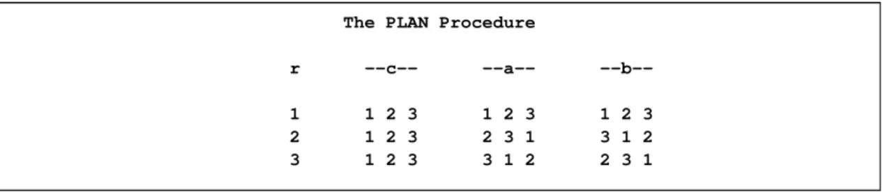
The following statements give an example of using both a FACTORS and a TREATMENTS statement. First theFACTORS statement sets up the rows and columns of a33square (factorsrandc). Then, the TREATMENTS statement augments the square with two cyclic treatments. The resulting design is a33

Graeco-Latin square, a type of design useful in main-effects factorial experiments. proc plan;

factors r=3 ordered c=3 ordered; treatments a=3 cyclic

b=3 cyclic 2; run;

The resulting Graeco-Latin square design is shown in Figure 67.5. Notice how the values ofr andcare ordered (1, 2, 3) as requested.

Figure 67.5 A33Graeco-Latin Square

r --c-- --a--

--b--1 1 2 3 1 2 3 1 2 3 2 1 2 3 2 3 1 3 1 2 3 1 2 3 3 1 2 2 3 1

Details: PLAN Procedure

Using PROC PLAN Interactively

After specifying a design with a FACTORSstatement and running PROC PLAN with a RUN statement, you can generate additional plans and output data sets without invoking PROC PLAN again.

In PROC PLAN, all statements can be used interactively. You can execute statements singly or in groups by following the single statement or group of statements with a RUN statement.

If you use PROC PLAN interactively, you can end the procedure with a DATA step, another PROC step, an ENDSAS statement, or a QUIT statement. The syntax of the QUIT statement is

(15)

Output Data Sets F 5597

When you use PROC PLAN interactively, additional RUN statements do not end the procedure but tell PROC PLAN to execute additional statements.

Output Data Sets

To understand how PROC PLAN creates output data sets, you need to look at how the procedure represents a plan. A plan is a list of values for all the factors, the values being chosen according to thefactor-selection

requests you specify. For example, consider the plan produced by the following statements: proc plan seed=12345;

factors a=3 b=2; run;

The plan as displayed by PROC PLAN is shown inFigure 67.6.

Figure 67.6 A Simple Plan

a 3 3 Random b 2 2 Random a -b-2 2 1 1 1 2 3 2 1

The first cell of the plan hasa=2 andb=2, the second has a=2 andb=1, the third hasa=1 andb=1, and so on. If you output the plan to a data set with the OUTPUT statement, by default the output data set contains a numeric variable with that factor’s name; the values of this numeric variable are the numbers of the successive levels selected for the factor in the plan. For example, the following statements produce

Figure 67.7.

proc plan seed=12345; factors a=3 b=2; output out=out; proc print data=out; run;

(16)

Figure 67.7 Output Data Set from Simple Plan Obs a b 1 2 2 2 2 1 3 1 1 4 1 2 5 3 2 6 3 1

Alternatively, you can specify the values that are output for a factor with theCVALS=orNVALS=option. Also, you can specify that the internal values be associated with the output values in random order with the

RANDOMoption. See the section “OUTPUT Statement” on page 5593.

If you also specify an input data set (DATA=), each factor is associated with a variable in theDATA=data set. This occurs either implicitly by the factor and variable having the same name or explicitly as described in the specifications for theOUTPUTstatement. In this case, the values of the variables corresponding to the factors are first read and then interpreted as describing the position of a cell in the plan. Then the respective values taken by the factors at that position are assigned to the variables in theOUT=data set. For example, consider the data set defined by the following statements.

data in; input a b; datalines; 1 1 2 1 3 1 ;

Suppose you specify this data set as an input data set for theOUTPUTstatement. proc plan seed=12345;

factors a=3 b=2;

output out=out data=in; proc print data=out;

run;

PROC PLAN interprets the first observation as referring to the cell in the first row and column of the plan, sincea=1 and b=1; likewise, the second observation is interpreted as the cell in the second row and first column, and the third observation as the cell in the third row and first column. In the output data set,aand

bhave the values they have in the plan at these positions, as shown inFigure 67.8.

Figure 67.8 Output Form of Input Data Set from Simple Plan Obs a b

1 2 2 2 1 1 3 3 2

(17)

Specifying Factor Structures F 5599

When the factors are random, this has the effect of randomizing the input data set in the same manner as the plan produced (see the sections “Randomizing Designs” on page 5601 and “Randomly Assigning Subjects to Treatments” on page 5588).

Specifying Factor Structures

By appropriately combining features of the PLAN procedure, you can construct an extensive set of designs. The basic tools are thefactor-selections, which are used in theFACTORSandTREATMENTSstatements.

Table 67.1summarizes how the procedure interprets variousfactor-selections(assuming that theORDERED

option is not specified in thePROC PLANstatement).

Table 67.1 Factor-SelectionInterpretation Form of

Request Interpretation Example Results

name=m produce a random per-mutation of the integers

1; 2; : : : ; m

t=15 lists a random order-ing of the numbers

1; 2; : : : ; 15

name=m

cyclic

cyclically permute the integers1; 2; : : : ; m

t=5 cyclic selects the integers 1 to 5. On the next iter-ation, selects 2,3,4,5,1; then 3,4,5,1,2; and so on.

name=mofn choose a random sample of m integers (with-out replacement) from the set of integers

1; 2; : : : ; n

t=5 of 15 lists a random selection of 5 numbers from 1 to 15. First, the proce-dure selects 5 numbers and then arranges them in random order.

name=mofn

ordered

has the same effect as

name=mordered

t=5 of 15 ordered

lists the integers 1 to 5 in increasing order (same as t=5 ordered)

name=mofn

cyclic

permutemof then inte-gers

t=5 of 30 cyclic

selects the integers 1 to 5. On the next iter-ation, selects 2,3,4,5,6; then 3,4,5,6,7; and so on. The 30th iteration produces 30,1,2,3,4; the 31st iteration produces 1,2,3,4,5; and so on.

(18)

Table 67.1 continued

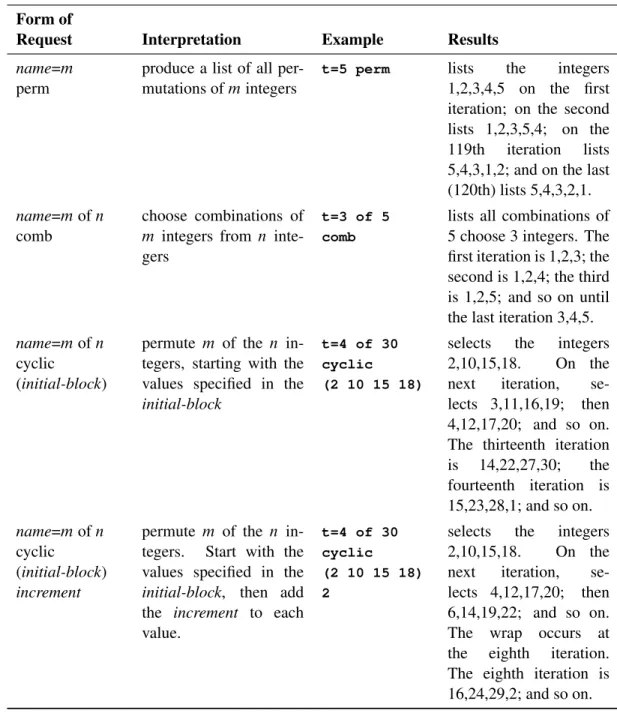
Form of

Request Interpretation Example Results

name=m

perm

produce a list of all per-mutations ofmintegers

t=5 perm lists the integers 1,2,3,4,5 on the first iteration; on the second lists 1,2,3,5,4; on the 119th iteration lists 5,4,3,1,2; and on the last (120th) lists 5,4,3,2,1.

name=mofn

comb

choose combinations of

m integers from n inte-gers

t=3 of 5 comb

lists all combinations of 5 choose 3 integers. The first iteration is 1,2,3; the second is 1,2,4; the third is 1,2,5; and so on until the last iteration 3,4,5.

name=mofn

cyclic

(initial-block)

permute m of the n in-tegers, starting with the values specified in the

initial-block

t=4 of 30 cyclic

(2 10 15 18)

selects the integers 2,10,15,18. On the next iteration, se-lects 3,11,16,19; then 4,12,17,20; and so on. The thirteenth iteration is 14,22,27,30; the fourteenth iteration is 15,23,28,1; and so on. name=mofn cyclic (initial-block) increment

permute m of the n in-tegers. Start with the values specified in the

initial-block, then add the increment to each value.

t=4 of 30 cyclic

(2 10 15 18) 2

selects the integers 2,10,15,18. On the next iteration, se-lects 4,12,17,20; then 6,14,19,22; and so on. The wrap occurs at the eighth iteration. The eighth iteration is 16,24,29,2; and so on.

InTable 67.1, in order for more than one iteration to appear in the plan, anothername=jfactor selection (withj > 1) must precede the example factor selection. For example, the following statements produce six of the iterations described in the last entry ofTable 67.1.

proc plan;

factors c=6 ordered t=4 of 30 cyclic (2 10 15 18) 2; run;

(19)

Randomizing Designs F 5601

proc plan ordered;

factors blocks=3 cell=5; treatments t=5 random; output out=rcdb;

run;

Randomizing Designs

In many situations, proper randomization is crucial for the validity of any conclusions to be drawn from an experiment. Randomization is used both to neutralize the effect of any unknown systematic biases that might be involved in the design and to provide a basis for the assumptions underlying the analysis.

You can use PROC PLAN to randomize an already existing design: one produced by a previous call to PROC PLAN, perhaps, or a more specialized design taken from a standard reference such asCochran and Cox(1957). The method is to specify the appropriate block structure in theFACTORSstatement and then to specify the data set where the design is stored with theDATA=option in theOUTPUTstatement. For an illustration of this method, see the section “Randomly Assigning Subjects to Treatments” on page 5588). Two sorts of randomization are provided for, corresponding to the RANDOM factor selection and associa-tion types in theFACTORSandOUTPUTstatements, respectively. Designs in which factors are completely nested (for example, block designs) should be randomized by specifying that the selection type of each fac-tor isRANDOMin theFACTORSstatement, which is the default (seeExample 67.3). On the other hand, if the factors are crossed (for example, row-and-column designs), they should be randomized by one random reassignment of their values for the whole design. To do this, specify that the association type of each factor isRANDOMin theOUTPUTstatement (seeExample 67.4).

Displayed Output

The PLAN procedure displays the following output:

themvalue for each factor, which is the number of values to be selected

thenvalue for each factor, which is the number of values to be selected from

the selection type for each factor, as specified in theFACTORSstatement

the initial block and increment number for cyclic factors

thefactor-value-selectionsmaking up each plan

In addition, notes are written to the log that give the starting and ending values of the random number seed for each call to PROC PLAN.

(20)

ODS Table Names

PROC PLAN assigns a name to each table it creates. You can use these names to reference the table in the Output Delivery System (ODS) to select tables and create output data sets. These names are listed in the following table. For more information about ODS, see Chapter 20, “Using the Output Delivery System.”

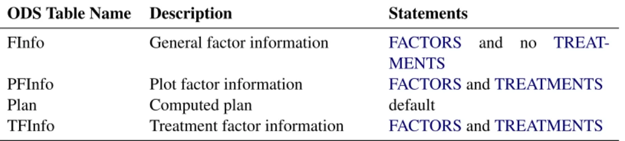
Table 67.2 ODS Tables Produced by PROC PLAN

ODS Table Name Description Statements

FInfo General factor information FACTORS and no TREAT-MENTS

PFInfo Plot factor information FACTORSandTREATMENTS

Plan Computed plan default

TFInfo Treatment factor information FACTORSandTREATMENTS

Examples: PLAN Procedure

Example 67.1: A Split-Plot Design

This plan is appropriate for a split-plot design with main plots forming a randomized complete block design. In this example, there are three blocks, four main plots per block, and two subplots per main plot. First, three random permutations (one for each of theblocks) of the integers 1, 2, 3, and 4 are produced. The four integers correspond to the four levels of the main plot factora; the permutation determines how the levels of a are assigned to the main plots within a block. For each of these 12 numbers (four numbers per block for three blocks), a random permutation of the integers 1 and 2 is produced. Each two-integer permutation determines the assignment of the two levels of the subplot factorb within a main plot. The following statements produceOutput 67.1.1:

title 'Split Plot Design'; proc plan seed=37277;

factors Block=3 ordered a=4 b=2; run;

(21)

Example 67.2: A Hierarchical Design F 5603

Output 67.1.1 A Split-Plot Design

Split Plot Design

Block 3 3 Ordered a 4 4 Random b 2 2 Random Block a -b-1 4 2 1 3 2 1 1 2 1 2 2 1 2 4 1 2 3 1 2 1 2 1 2 1 2 3 4 2 1 2 2 1 3 2 1 1 2 1

Example 67.2: A Hierarchical Design

In this example, three plants are nested within four pots, which are nested within three houses. The FAC-TORSstatement requests a random permutation of the numbers 1, 2, and 3 to chooseHousesrandomly. The second step requests a random permutation of the numbers 1, 2, 3, and 4 for each of those first three numbers to randomly assignPotstoHouses. Finally, theFACTORSstatement requests a random permu-tation of 1, 2, and 3 for each of the 12 integers in the second set of permupermu-tations. This last step randomly assignsPlantstoPots. The following statements produceOutput 67.2.1:

title 'Hierarchical Design'; proc plan seed=17431;

factors Houses=3 Pots=4 Plants=3 / noprint; output out=nested;

run;

proc print data=nested; run;

(22)

Output 67.2.1 A Hierarchical Design

Hierarchical Design

Obs Houses Pots Plants

1 1 3 2 2 1 3 3 3 1 3 1 4 1 1 3 5 1 1 1 6 1 1 2 7 1 2 2 8 1 2 3 9 1 2 1 10 1 4 3 11 1 4 2 12 1 4 1 13 2 4 1 14 2 4 3 15 2 4 2 16 2 2 2 17 2 2 1 18 2 2 3 19 2 3 2 20 2 3 3 21 2 3 1 22 2 1 2 23 2 1 3 24 2 1 1 25 3 4 1 26 3 4 3 27 3 4 2 28 3 1 3 29 3 1 2 30 3 1 1 31 3 2 1 32 3 2 2 33 3 2 3 34 3 3 3 35 3 3 2 36 3 3 1

Example 67.3: An Incomplete Block Design

Jarrett and Hall(1978) give an example of a generalized cyclic design with good efficiency characteristics. The design consists of two replicates of 52 treatments in 13 blocks of size 8. The following statements use the PLAN procedure to generate this design in an appropriately randomized form and store it in a SAS data setGCBD. Then the design is sorted and transposed to display in randomized order. The following statements produceOutput 67.3.1andOutput 67.3.2:

(23)

Example 67.3: An Incomplete Block Design F 5605

title 'Generalized Cyclic Block Design'; proc plan seed=33373;

treatments Treatment=8 of 52 cyclic (1 2 3 4 32 43 46 49) 4; factors Block=13 Plot=8;

output out=GCBD; quit;

proc sort data=GCBD out=GCBD; by Block Plot;

proc transpose data= GCBD(rename=(Plot=_NAME_)) out =tGCBD(drop=_NAME_);

by Block; var Treatment;

proc print data=tGCBD noobs; run;

Output 67.3.1 A Generalized Cyclic Block Design

Generalized Cyclic Block Design

Plot Factors

Block 13 13 Random Plot 8 8 Random

Factor Select Levels Order Initial Block / Increment

Treatment 8 52 Cyclic (1 2 3 4 32 43 46 49) / 4

Block ---Plot---

---Treatment---10 7 4 8 1 2 3 5 6 1 2 3 4 32 43 46 49 8 1 2 4 3 8 6 5 7 5 6 7 8 36 47 50 1 9 2 5 4 7 3 1 8 6 9 10 11 12 40 51 2 5 6 4 2 6 8 3 7 1 5 13 14 15 16 44 3 6 9 7 4 7 6 3 1 2 8 5 17 18 19 20 48 7 10 13 4 4 8 1 5 3 6 7 2 21 22 23 24 52 11 14 17 2 6 2 3 8 7 5 1 4 25 26 27 28 4 15 18 21 3 6 2 3 1 7 4 5 8 29 30 31 32 8 19 22 25 1 1 2 7 8 5 6 3 4 33 34 35 36 12 23 26 29 5 5 7 6 8 4 3 1 2 37 38 39 40 16 27 30 33 12 5 8 1 4 7 3 6 2 41 42 43 44 20 31 34 37 13 3 5 1 8 4 2 6 7 45 46 47 48 24 35 38 41 11 4 1 5 2 3 8 6 7 49 50 51 52 28 39 42 45

(24)

Output 67.3.2 A Generalized Cyclic Block Design

Generalized Cyclic Block Design

Block _1 _2 _3 _4 _5 _6 _7 _8 1 33 34 26 29 12 23 35 36 2 18 26 27 21 15 25 4 28 3 32 30 31 19 22 29 8 25 4 23 17 52 21 24 11 14 22 5 30 33 27 16 37 39 38 40 6 6 14 44 13 9 15 3 16 7 48 7 20 17 13 19 18 10 8 5 6 8 7 50 47 1 36 9 51 9 40 11 10 5 12 2 10 4 32 43 2 46 49 1 3 11 50 52 28 49 51 42 45 39 12 43 37 31 44 41 34 20 42 13 47 35 45 24 46 38 41 48

Example 67.4: A Latin Square Design

All of the preceding examples involve designs with completely nested block structures, for which PROC PLAN was especially designed. However, by appropriate coordination of its facilities, a much wider class of designs can be accommodated. A Latin square design is based on experimental units that have a row-and-column block structure. The following example uses theCYCLICoption for a treatment factortmts

to generate a simple44Latin square. Randomizing a Latin square design involves randomly permuting the row, column, and treatment values independently. In order to do this, use the RANDOMoption in the OUTPUT statement of PROC PLAN. The example also uses factor-value-settings in the OUTPUT

statement. The following statements produceOutput 67.4.1: title 'Latin Square Design';

factors Row=4 ordered Col=4 ordered / noprint; treatments Tmt=4 cyclic;

output out=LatinSquare

Row cvals=('Day 1' 'Day 2' 'Day 3' 'Day 4') random Col cvals=('Lab 1' 'Lab 2' 'Lab 3' 'Lab 4') random Tmt nvals=( 0 100 250 450) random; quit;

proc sort data=LatinSquare out=LatinSquare; by Row Col;

proc transpose data= LatinSquare(rename=(Col=_NAME_)) out =tLatinSquare(drop=_NAME_);

by Row; var Tmt;

proc print data=tLatinSquare noobs; run;

(25)

Example 67.5: A Generalized Cyclic Incomplete Block Design F 5607

Output 67.4.1 A Randomized Latin Square Design Latin Square Design

Row Lab_1 Lab_2 Lab_3 Lab_4

Day 1 0 250 100 450 Day 2 250 450 0 100 Day 3 100 0 450 250 Day 4 450 100 250 0

Example 67.5: A Generalized Cyclic Incomplete Block Design

The following statements depict how to create an appropriately randomized generalized cyclic incomplete block design forv treatments (given by the value oft) inb blocks (given by the value ofb) of sizek(with values ofpindexing the cells within a block) with initial block.e1e2 ek/and increment numberi.

factors b=bp=k;

treatments t=kofvcyclic (e1e2 ek )i ;

For example, the specification proc plan seed=37430;

factors b=10 p=4;

treatments t=4 of 30 cyclic (1 3 4 26) 2; run;

generates the generalized cyclic incomplete block design given in Example 1 of Jarrett and Hall(1978), which is given by the rows and columns of the plan associated with the treatment factortinOutput 67.5.1.

Output 67.5.1 A Generalized Cyclic Incomplete Block Design The PLAN Procedure

Plot Factors

b 10 10 Random

p 4 4 Random

Initial Block Factor Select Levels Order / Increment

(26)

Output 67.5.1 continued b ---p--- ---t---2 2 3 1 4 1 3 4 26 1 3 2 4 1 3 5 6 28 3 2 3 4 1 5 7 8 30 10 4 2 3 1 7 9 10 2 9 4 1 2 3 9 11 12 4 4 1 3 2 4 11 13 14 6 5 1 2 4 3 13 15 16 8 8 3 2 4 1 15 17 18 10 7 2 4 1 3 17 19 20 12 6 2 1 4 3 19 21 22 14

Example 67.6: Permutations and Combinations

Occasionally, you might need to generate all possible permutations ofnthings, or all possible combinations ofnthings takenmat a time.

For example, suppose you are planning an experiment in cognitive psychology where you want to present four successive stimuli to each subject. You want to observe each permutation of the four stimuli. The following statements use PROC PLAN to create a data set containing all possible permutations of four numbers in random order.

title 'All Permutations of 1,2,3,4'; proc plan seed=60359;

factors Subject = 24

Order = 4 ordered; treatments Stimulus = 4 perm; output out=Psych;

run;

proc sort data=Psych out=Psych; by Subject Order;

proc transpose data= Psych(rename=(Order=_NAME_)) out =tPsych(drop=_NAME_);

by Subject; var Stimulus;

proc print data=tPsych noobs; run;

The variableSubjectis set at 24 levels because there are4Š_D24total permutations to be listed. IfSubject> 24, the list repeats. Output 67.6.1displays the PROC PLAN output. Note that the variableSubjectis listed in random order.

(27)

Example 67.6: Permutations and Combinations F 5609

Output 67.6.1 List of Permutations

All Permutations of 1,2,3,4

Plot Factors

Subject 24 24 Random Order 4 4 Ordered

Stimulus 4 4 Perm

Subject -Order-

-Stimulus-4 1 2 3 4 1 2 3 4 15 1 2 3 4 1 2 4 3 24 1 2 3 4 1 3 2 4 1 1 2 3 4 1 3 4 2 5 1 2 3 4 1 4 2 3 17 1 2 3 4 1 4 3 2 19 1 2 3 4 2 1 3 4 14 1 2 3 4 2 1 4 3 6 1 2 3 4 2 3 1 4 23 1 2 3 4 2 3 4 1 8 1 2 3 4 2 4 1 3 2 1 2 3 4 2 4 3 1 13 1 2 3 4 3 1 2 4 16 1 2 3 4 3 1 4 2 12 1 2 3 4 3 2 1 4 18 1 2 3 4 3 2 4 1 21 1 2 3 4 3 4 1 2 9 1 2 3 4 3 4 2 1 22 1 2 3 4 4 1 2 3 10 1 2 3 4 4 1 3 2 7 1 2 3 4 4 2 1 3 11 1 2 3 4 4 2 3 1 3 1 2 3 4 4 3 1 2 20 1 2 3 4 4 3 2 1

The output data setPsychcontains 96 observations of the 3 variables (Subject,Order, andStimulus). Sorting the output data set bySubjectand byOrderwithinSubjectresults in all possible permutations ofStimulus

(28)

Output 67.6.2 Randomized Permutations All Permutations of 1,2,3,4 Subject _1 _2 _3 _4 1 1 3 4 2 2 2 4 3 1 3 4 3 1 2 4 1 2 3 4 5 1 4 2 3 6 2 3 1 4 7 4 2 1 3 8 2 4 1 3 9 3 4 2 1 10 4 1 3 2 11 4 2 3 1 12 3 2 1 4 13 3 1 2 4 14 2 1 4 3 15 1 2 4 3 16 3 1 4 2 17 1 4 3 2 18 3 2 4 1 19 2 1 3 4 20 4 3 2 1 21 3 4 1 2 22 4 1 2 3 23 2 3 4 1 24 1 3 2 4

As another example, suppose you have six alternative treatments, any four of which can occur together in a block (in no particular order). The following statements use PROC PLAN to create a data set containing all possible combinations of six numbers taken four at a time. In this case, you use ODS to create the data set.

title 'All Combinations of (6 Choose 4) Integers'; proc plan;

factors Block=15 ordered Treat= 4 of 6 comb; ods output Plan=Combinations; run;

proc print data=Combinations noobs; run;

The variable Blockhas 15 levels since there are a total of6Š=.4Š2Š/ _D 15 combinations of four integers chosen from six integers. The data set formed by ODS from the displayed plan has one row for each block, with the four values ofTreatcorresponding to four different variables, as shown inOutput 67.6.3and

(29)

Example 67.6: Permutations and Combinations F 5611

Output 67.6.3 List of Combinations

All Combinations of (6 Choose 4) Integers

Block 15 15 Ordered Treat 4 6 Comb Block -Treat-1 1 2 3 4 2 1 2 3 5 3 1 2 3 6 4 1 2 4 5 5 1 2 4 6 6 1 2 5 6 7 1 3 4 5 8 1 3 4 6 9 1 3 5 6 10 1 4 5 6 11 2 3 4 5 12 2 3 4 6 13 2 3 5 6 14 2 4 5 6 15 3 4 5 6

Output 67.6.4 Combinations Data Set Created by ODS

All Combinations of (6 Choose 4) Integers

Block Treat1 Treat2 Treat3 Treat4

1 1 2 3 4 2 1 2 3 5 3 1 2 3 6 4 1 2 4 5 5 1 2 4 6 6 1 2 5 6 7 1 3 4 5 8 1 3 4 6 9 1 3 5 6 10 1 4 5 6 11 2 3 4 5 12 2 3 4 6 13 2 3 5 6 14 2 4 5 6 15 3 4 5 6

(30)

Example 67.7: Crossover Designs

Incrossoverexperiments, the same experimental units or subjects are given multiple treatments in sequence, and the model for the response at any one period includes an effect for the treatment applied in the previous period. A good design for a crossover experiment is therefore one that balances how often each treatment is preceded by each other treatment. Cox (1992) gives the following example of a balanced crossover experiment for paper production. In this experiment, the subjects are production runs of the mill, with the treatments being six different concentrations of pulp used in sequence. The following statements construct this design in a standard form:

proc plan;

factors Run=6 ordered Period=6 ordered; treatments Treatment=6 cyclic (1 2 6 3 5 4); run;

Output 67.7.1shows the results of the preceding statements.

Output 67.7.1 Crossover Design for Six Treatments The PLAN Procedure

Plot Factors

Run 6 6 Ordered

Period 6 6 Ordered

Initial Block Factor Select Levels Order / Increment

Treatment 6 6 Cyclic (1 2 6 3 5 4) / 1

Run ---Period--

-Treatment-1 1 2 3 4 5 6 1 2 6 3 5 4 2 1 2 3 4 5 6 2 3 1 4 6 5 3 1 2 3 4 5 6 3 4 2 5 1 6 4 1 2 3 4 5 6 4 5 3 6 2 1 5 1 2 3 4 5 6 5 6 4 1 3 2 6 1 2 3 4 5 6 6 1 5 2 4 3

The construction method for this example is due toWilliams (1949). The initial block for the treatment variableTreatmentis defined as follows forn_D6:

(31)

Example 67.7: Crossover Designs F 5613

This general form serves to generate a balanced crossover design forntreatments andnsubjects innperiods whennis even. Whennis odd,2nsubjects are required, with the following initial blocks, respectively for odd and evenn:

.1 2 n 3 n 1 : : : n=2_C1 n=2/ .n=2 n=2_C1 : : : n 1 3 n 2 1/

In order to randomize Williams’ crossover designs, the following statements randomly permute the subjects and treatments:

factors Run=6 ordered Period=6 ordered / noprint; treatments Treatment=6 cyclic (1 2 6 3 5 4); output out=RandomizedDesign

Run random Treatment random ;

/*

/ Relabel Period to obtain the same design as in Cox (1992).

/---*/ data RandomizedDesign; set RandomizedDesign;

Period = mod(Period+2,6)+1; run;

proc sort data=RandomizedDesign; by Run Period;

proc transpose data=RandomizedDesign out=tDesign(drop=_name_); by notsorted Run;

var Treatment;

data tDesign; set tDesign;

rename COL1-COL6 = Period_1-Period_6; proc print data=tDesign noobs;

run;

In the preceding statements,RunandTreatmentare randomized by using theRANDOMoption in the OUT-PUTstatement, and new labels forPeriodare obtained in a subsequent DATA step. ThisPeriodrelabeling is not necessary and might not be valid for Williams’ designs in general; it is used in this example only to match results with those ofCox(1992). The SORT and TRANSPOSE steps then prepare the design to be printed in a standard form, shown inOutput 67.7.2.

Output 67.7.2 Randomized Crossover Design

Run Period_1 Period_2 Period_3 Period_4 Period_5 Period_6

1 3 6 2 5 4 1 2 5 3 4 6 1 2 3 1 4 5 2 6 3 4 2 1 6 4 3 5 5 6 5 1 3 2 4 6 4 2 3 1 5 6

(32)

The analysis of a crossover experiment requires for each observation a carryover variable whose values are the treatment in the preceding period. The following statements add such a variable to the randomized design constructed previously:

proc sort data=RandomizedDesign; by Run Period;

data RandomizedDesign; set RandomizedDesign; by Run period;

LagTreatment = lag(Treatment);

if (first.Run) then LagTreatment = .; run;

proc transpose data=RandomizedDesign out=tDesign(drop=_name_); by notsorted Run;

var LagTreatment; data tDesign; set tDesign;

rename COL1-COL6 = Period_1-Period_6; proc print data=tDesign noobs;

run;

Output 67.7.3displays the values of the carryover variable for each run and period.

Output 67.7.3 Lag Treatment Effect in Crossover Design

Run Period_1 Period_2 Period_3 Period_4 Period_5 Period_6

1 . 3 6 2 5 4 2 . 5 3 4 6 1 3 . 1 4 5 2 6 4 . 2 1 6 4 3 5 . 6 5 1 3 2 6 . 4 2 3 1 5

Of course, the carryover variable has no effect in the first period, which is why it is coded with a missing value in this case.

The experimental LAG effect in the EFFECT statement in PROC ORTHOREG provides a convenient mech-anism for incorporating the carryover effect into the analysis. The following statements first add the ob-served data to the design to create theMillsdata set. Then PROC ORTHOREG is invoked, and the carryover effect is defined as a lag effect with the relevant period and subject information specified. ODS is used to trim down the results to show only the parts that are usually of interest in crossover analysis. For more information about the EFFECTS statement in PROC ORTHOREG, see the section “EFFECT Statement” on page 5344. data Responses; input Response @@; datalines; 56.7 53.8 54.4 54.4 58.9 54.5 58.5 60.2 61.3 54.4 59.1 59.8 55.7 60.7 56.7 59.9 56.6 59.6 57.3 57.7 55.2 58.1 60.2 60.2 53.7 57.1 59.2 58.9 58.9 59.6 58.1 55.7 58.9 56.6 59.6 57.5 ;

(33)

Example 67.7: Crossover Designs F 5615

data Mills;

merge RandomizedDesign Responses; run;

proc orthoreg data=Mills; class Run Period Treatment;

effect CarryOver = lag(Treatment / period=Period within=Run); model Response = Run Period Treatment CarryOver;

test Run Period Treatment CarryOver / htype=1; lsmeans Treatment CarryOver / diff=anom;

ods select Tests1 LSMeans Diffs; run;

Output 67.7.4shows the carryover analysis that results from the preceding statements.

Output 67.7.4 Carryover Analysis for Crossover Experiment The ORTHOREG Procedure

Dependent Variable: Response

Type I Tests of Model Effects

Num Den Effect DF DF F Value Pr > F Run 5 15 13.76 <.0001 Period 5 15 7.19 0.0013 Treatment 5 15 22.95 <.0001 CarryOver 5 15 7.76 0.0009

Treatment Least Squares Means

Standard

Treatment Estimate Error DF t Value Pr > |t|

1 57.1954 0.3220 15 177.65 <.0001 2 57.6204 0.3220 15 178.97 <.0001 3 59.1919 0.3220 15 183.85 <.0001 4 59.2288 0.3220 15 183.97 <.0001 5 57.9829 0.3220 15 180.10 <.0001 6 55.0639 0.3220 15 171.03 <.0001

Differences of Treatment Least Squares Means

Standard

Treatment _Treatment Estimate Error DF t Value Pr > |t|

1 Avg -0.5185 0.2948 15 -1.76 0.0990 2 Avg -0.09345 0.2948 15 -0.32 0.7556 3 Avg 1.4780 0.2948 15 5.01 0.0002 4 Avg 1.5149 0.2948 15 5.14 0.0001 5 Avg 0.2690 0.2948 15 0.91 0.3758 6 Avg -2.6500 0.2948 15 -8.99 <.0001

(34)

Output 67.7.4 continued

CarryOver Least Squares Means

Carry Standard

Over Estimate Error DF t Value Pr > |t|

1 Non-est . . . . 2 Non-est . . . . 3 Non-est . . . . 4 Non-est . . . . 5 Non-est . . . . 6 Non-est . . . .

Differences of CarryOver Least Squares Means

_

Carry Carry Standard

Over Over Estimate Error DF t Value Pr > |t|

1 Avg 0.3726 0.3284 15 1.13 0.2743 2 Avg -0.2774 0.3284 15 -0.84 0.4116 3 Avg 0.6512 0.3284 15 1.98 0.0660 4 Avg -1.3274 0.3284 15 -4.04 0.0011 5 Avg 1.3976 0.3284 15 4.26 0.0007 6 Avg -0.8167 0.3284 15 -2.49 0.0252

The Type I analysis of variance indicates that all effects are significant—in particular, both the direct and the carryover effects of the treatment. In the presence of carryover effects, the LS-means need to be defined with some care. The LS-means for treatments computed using balanced margins for the carryover effect are inestimable; so the OBSMARGINS option is specified in the LSMEANS statement in order to use the observed margins instead. The observed margins take the absence of a carryover effect in the first period into account. Note that the LS-means themselves of the carryover effect are inestimable, but their differences are estimable. The LS-means of the direct effect of the treatment and the ANOM differences for the LS-means of their carryover effect match the “adjusted direct effects” and “adjusted residual effects,” respectively, of

Cox(1992).

References

Cochran, W. G. and Cox, G. M. (1957),Experimental Designs, Second Edition, New York: John Wiley & Sons.

Cox, D. R. (1992), Planning of Experiments, Wiley Classics Library Edition, New York: John Wiley & Sons.

Jarrett, R. G. and Hall, W. B. (1978), “Generalized Cyclic Incomplete Block Designs,” Biometrika, 65, 397–401.

Williams, E. J. (1949), “Experimental Designs Balanced for the Estimation of Residual Effects of Treat-ments,”Australian Journal of Scientific Research, Series A, 2, 149–168.

(35)

Subject Index

C

combinations

generating with PLAN procedure,5608

crossover designs

analyzing with GLIMMIX procedure,5612

D

design of experiments,seeexperimental design

E

experimental design,see alsoPLAN procedure

F

factors

PLAN procedure,5590,5591,5599

G

generalized cyclic incomplete block design

GLIMMIX procedure

crossover designs,5612

Graeco-Latin square

H

hierarchical design

I

incomplete block design

generating with PLAN procedure,5604,5607

L

Latin square design

N

nested design

P

permutation

PLAN procedure

combinations,5608

compared to other procedures,5586

crossover designs,5612

factor, selecting levels for,5590,5591

generalized cyclic incomplete block design,5607

hierarchical design,5603

incomplete block design,5604,5607

input data sets,5590,5593

introductory example,5587

Latin square design,5606

nested design,5603

ODS table names,5602

output data sets,5590,5593,5597,5598

permutations,5608

random number generators,5590

randomizing designs,5598,5601

specifying factor structures,5599

split-plot design,5602

treatments, specifying,5595

using interactively,5596 R

random number generators

PLAN procedure,5590

randomization of designs

using PLAN procedure,5601

S

split-plot design

T

treatments in a design

(36)

(37)

Syntax Index

C

CVALS= option

OUTPUT statement (PLAN),5594

F

factor-value-settings option

FACTORS statement

PLAN procedure,5590

N

NOPRINT option

FACTOR statement (PLAN),5591

NVALS= option

O

ORDERED option

PROC PLAN statement,5590

OUT= option

OUTPUT statement PLAN procedure,5593 P PLAN procedure factor-value-setting specification,5594,5595 syntax,5590

PLAN procedure, FACTOR statement

NOPRINT option,5591

PLAN procedure, FACTORS statement,5590

PLAN procedure, OUTPUT statement,5593

CVALS= option,5594 factor-value-settings option,5594 NVALS= option,5594 ORDERED option,5594 OUT= option,5593 RANDOM option,5594

PLAN procedure, PROC PLAN statement,5590

ORDERED option,5590

SEED option,5590

PLAN procedure, TREATMENTS statement,5595

PROC PLAN statement,seePLAN procedure

R

RANDOM option

S

SEED option

PROC PLAN statement,5590

T

TREATMENTS statement

(38)

(39)

Your Turn

We welcome your feedback.

If you have comments about this book, please send them to

[email protected]. Include the full title and page numbers (if applicable).

If you have comments about the software, please send them to [email protected].

(40)