[Type here] [Type here]
=]
Optimisation of Run of River
Production
Forecasting
Using
Aiolos Forecast Studio
________________________________________________
Amer Al-Qes
Master Thesis
TVVR 20/5012
Division of Water Resources Engineering
Department of Building and Environmental Technology Lund University
Trading and Asset Optimisation Generation Division
i
Optimisation of Run of River Production
Forecasting Using Aiolos Forecast Studio
By: Amer Al-Qes
Master Thesis
Division of Water Resources Engineering
Department of Building & Environmental Technology Lund University
Box 118
ii Water Resources Engineering
TVVR-20/5012 ISSN 1101-9824 Lund 2020 www.tvrl.lth.se
i Master Thesis
Division of Water Resources Engineering
Department of Building & Environmental Technology Lund University
English title: Optimisation of Run of River Production Forecasting Using Aiolos Forecast Studio
Author(s): Amer Al-Qes Supervisor: Magnus Persson
Joakim Henriksson Examiner: Cintia Bertacchi Uvo
Language English
Year: 2020
Keywords: Run of river hydropower plants, power production forecasting, Aiolos forecast studio, model accuracy assessment analysis and power market.
ii
Acknowledgements
Foremost, I would like to express my gratitude and delight to carry out this study at Forum. Where my supervisor Joakim Henriksson and my thesis manager Hans Bjerhag provided me with support, knowledge, and resources during this study, therefore I would like to express my sincere thanks to them. I have also had the privilege to work on Aiolos Forecast Studio developed by Vitec. I thank Vitec personal Christer Modin and Magnus Fohlman, who contributed significantly to my understanding of the program and discussed the applicability of my recommendations.
I would also like to thank the staff of Lund University for the knowledge and support they provided during my master study, as well as my thesis supervisor Magnus Persson for his help and guidance.
Finally I would like to thank my family and my friends, for encouraging me and giving me all the support that I need.
Abstract
This report investigates the performance of Aiolos Forecast Studio (AFS) in forecasting hydropower production by comparing the computed power production and runoff with the historical ones. Several statistical tools are used to assess the performance and accuracy of the models, which were also essential for deriving results and conclusions of this study. At first, two hydropower stations are taken as a case study (Holmen and Jordalen 2) which are in Norway and run by Småkraft. Said hydropower stations lie in the same watershed (Jordalselvi) in succession to each other on the same river. Furthermore, for validating the findings of this report, five more hydropower stations are chosen. The approach was to achieve an in-depth understanding of the program, followed by developing a recalibration procedure to enhance the production forecasts accuracy. Some limitations prevent the production forecast from attaining a higher level of accuracy; however, this report analyses those limitations thoroughly and provides recommendations for surpassing them. Overall coupled with the recalibration procedure, AFS has proven to be a reliable tool in Hydropower production forecasting.
iv
Symbols and Abbreviations
ROR Run of River P Power
RORs Run of river
hydropower stations
ρ Water mass density
𝑔 Gravitational acceleration TSO Transmission System
Operator Q Flow H Water head HBV Hydrologiska Byråns Vattenbalansavdelning 𝜂 Turbine efficiency NSEC Nash-Sutcliffe Efficiency Coefficient Qs Surface Runoff HSPF Hydrological Simulation Program - FORTRAN ET Evapotranspiration ΔG W
Change in groundwater storage
AFS Aiolos Forecast Studio Pr Precipitation GIS Geographical
information system
ΔS Change in storage due to snow cover
RMSE Root mean square error ΔS M
Change in soil moisture storage MAE Mean absolute error t Time
ME Mean error k Decay constant
NRMSE Normalized RMSE fc Minimum infiltration rate r Runoff factor
v f0 Maximum (initial)
infiltration rate
fp Potential infiltration rate
R Runoff Qe Vapour condensation energy
ΔM Other change in water storage volume (ground, lakes and groundwater)
Qg Energy conduction from ground Qp Energy conducted from rainfall
E Evaporation ΔQi Rate of change in the internal energy stored in the snow αMP average forecasted
production at hour t
Ql Total shortwave energy emitted by the snow
βH(t) The sensitivity for differences in the runoff
B Thermal quality of the snow
yi Measured data A Albedo
ŷi or fi Computed data li Daily incident solar radiation ӯi The arithmetic mean of
the measured data
Ts Blackbody temperature (snow surface temperature)
N or n Number of values σ Stefan-Blotzman constant Qm The total energy
available for snowmelt
Dh Bulk transfer coefficient for sensible heat transfer Qsn Net shortwave radiation De Bulk transfer coefficient for
latent heat transfer
Qln Net long-wave radiation uz Wind speed at a chosen height above the snow surface
Qc Convection from air Ta The temperature at the air surface
vi ea Vapour pressure of the
air surface
es Vapour pressure of the snow surface
vii
Contents
1 Introduction ... 1
2 Background ... 2
2.1 ROR Hydropower Generation ... 2
2.1.1 Hydropower ... 2
2.1.2 ROR Hydropower Stations ... 4
2.2 Deregulated power markets ... 5
2.2.1 Day-Ahead and Real-Time Market ... 5
2.3 Hydropower production forecasting ... 7
2.4 Rainfall-runoff modelling ... 7
2.4.1 Conceptual model ... 8
2.4.2 Spatial Processes ... 9
3 Theory ... 10
3.1 The hydrologic cycle and surface runoff ... 10
3.2 Linear Regression (statistical model) ... 12
3.3 Nash-Sutcliffe Efficiency Coefficient ... 13
3.4 Aiolos Forecast Studio and The Achelous model ... 14
3.4.1 Achelous Hydrological Component ... 16
3.4.2 Achelous basin properties ... 21
3.4.3 Achelous statistical component ... 22
3.4.4 Aiolos Forecast Studio built-in evaluation tools. ... 27
3.5 ArcMap (GIS) ... 28
4 Delimitations, limitations and Assumptions ... 29
5 Preliminary Model Accuracy Assessment ... 30
viii
5.2 Procedure and Results ... 30
6 Recalibration ... 33
6.1 Improving the runoff forecast accuracy ... 35
6.1.1 Altitude ... 37
6.1.2 Forest canopy ... 38
6.1.3 Maximum storage and Discharge rate ... 40
6.2 Improving the power production forecast accuracy ... 41
7 Results and Discussion ... 43
8 Conclusions and Recommendations ... 51
1
1
Introduction
Production forecasting is an essential tool for power companies, that facilitates bidding in the power market, as well as for power stations operation. In this report AFS is adopted as a tool for forecasting power production; it consists of several models simulating power production from various power sources. The most relevant model is the Achelous, which is the hydropower model in AFS, specialised in unregulated hydropower production forecasting. The Achelous model comprises a hydrological model and a statistical model that use the weather forecast and historical data as input. Those two models work simultaneously to produce the most accurate result (Vitec Energy AB, 2020). Run-of-river (ROR) hydropower stations have regulating structures with little water storage capacity on the upstream side, making it challenging to regulate the streamflow in dry periods. Therefore, produce power depending on the river flow regime, which is also why RORs can be unreliable as the primary power source. RORs can provide financial benefits for small communities as well. As an example, Småkraft (a power company in Norway) operates 112 ROR power stations across Norway that created job opportunities, provided income for landowners, and tax funds for local municipalities (Smakraft, 2019).
2
2
Background
Models are created to simulate an actual process or phenomena as accurately as possible. There are many applications for models, but in this case, the model is used to accurately forecast the hydropower production, to optimise power production and market bidding. There are several statistical tools used to assess the accuracy of a model, for simplicity and ease of interpretation the most relevant were chosen and applied. The Nash-Sutcliffe Coefficient and the Deviation of the Runoff Volumes are the two criteria (tools) used to assess the model.
Typically, hydropower is planned and run based on a complete optimisation using price forecasting and water availability. Production planning is often done manually using optimisation tools tailored to the company's overall business image, which can be time-consuming and more susceptible to error. A computer model can replace the manual procedure to provide higher efficiency and more accurate forecasts. The model shall comprise algorithms for forecasting runoff power production and power consumption.
2.1
ROR Hydropower Generation
Run of river hydropower station is a term used to describe hydropower stations with limited regulation to the river flow since it usually holds little or no storage on the upstream part of the river. Thus, given the name Run of River since the power generation is controlled mostly by the hydrological conditions of the river watershed. (Helston, 2017).
2.1.1 Hydropower
Hydropower is an environmentally friendly and sustainable form of power generation; the water mechanics and behaviour fuel it in a watershed.
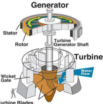
Hydropower is generated through harnessing the kinetic and potential energy of the streamflow and converting it to mechanical energy by running the water through the turbine blades setting the turbine into rotational motion. The turbine is centred around a shaft perpendicular to the blades motion direction which transfers the mechanical torque to the generator, which in turn converts the mechanical energy into electrical energy. Figure 1 shows a simplified model of a hydropower generator (USBR Power Resources Office, 2005).
3
Figure 1 Simple hydropower generator sketch (USGS, 2018)
𝑃 = 𝜂𝜌𝑔𝑄𝐻 (1)
Equation 1 The governing equation for calculating hydropower, where; P = power (MW)
η = turbine efficiency
ρ = water mass density (kg/m3)
Q = discharge (m3/s)
g = gravity (9.82 m/s2)
H = hydraulic head (m). (Oregon State University, 2020)
From Equation 1, it is clear that the significant factors in determining the power production are the inflow volume and the water head. Depending on the topography of the watershed, a large dam can be built to remarkably increase the water head and enhance the storage capabilities (for seasonal production control). While for ROR hydropower stations, a regulating hydraulic structure is constructed to control the power production and in turn raise the water head.
4
2.1.2 ROR Hydropower Stations
ROR is usually composed of three main parts an intake structure, powerhouse and an outlet as seen in (Figure 2). Those three main parts vary in their design and composition, depending on several determining factors, for instance; water head, generation capacity and river conditions. In the upstream part of the structure lies the water intake which redirects water from the stream or reservoir into the turbine through an inlet fitted with screens to filter the debris and large sediments. When the inlet structure is located further upstream the hydropower station, the water is transported through a penstock, which acts like a pipe connecting the inlet structure to the turbine, as shown in Figure 2. Finally, the water is discharged back to the stream through an outlet.
Figure 2 Simple sketch for a run of river hydropower station (Scottish Government, 2020)
Due to their small storage capacity, it is viable for ROR hydropower stations to have accurate forecasts that integrate them into a power production grid which serves to be both energies efficient and economically feasible. (USGS, 2018).
5
2.2
Deregulated power markets
Power markets are mainly composed of three main sectors production, transmission, and distribution. Traditionally those sectors were controlled by large often state-owned monopolies, but in the past decades, many markets became deregulated. Several approaches achieved deregulation, but its main aim was to stimulate competition, to achieve lower retail prices for the consumer side. The deregulation began by the split of vertically integrated power producers and privatised state-owned utilities, in other words, the transmission sector was separated from the production and distribution as an independent system operator currently known as TSO (transmission system operator). Despite the deregulations, the electrical grid is still heavily regulated to ensure the balance between production and demand. In many countries, wholesale markets were established where the power producers could sell their generated electricity, considering the grid connection and the need to balance the supply and demand instantly. As a result of deregulation two basic models for power, markets were developed: power pools and power exchanges. The power pools are the one where the trading, dispatch and transmission takes place at the system operators' side. While at the power markets, trading and initial dispatch take place at power exchanges which are independent of the transmission. In the Nordic countries, the power pool model is used, where the system operators are responsible for estimating the power demand, receiving bids from power producers, and calculating the pricing. Moreover, TSO mainly ensures the balance in the power grid by continually monitoring the balance between the supply and demand.
Several electrical markets exist all around the world, from which some are regional (local), and some are international, which involve power trading among multiple countries. The Nordic market is an example of an international market; in other means, electrical power produced in one country can be sold to another (Mayer & Trück, 2018).
2.2.1 Day-Ahead and Real-Time Market
The day-ahead market (also referred to as intra-day) allows the participants to prepare their bids for buying and selling power and services day ahead of the sale. The day-ahead market bidding takes place in power pools; for the Nordic
6
market, the power pool is called Xbid and managed by Nord pool. The system operators (TSO) give out information and forecasts regarding the next day, which helps the participants in optimising their production and formulating their bids for the power company's dispatchers to make the sales. Production and consumption forecasting are crucial in this type of market, mainly because it involves selling a large amount of power. The real-time market functions differently, the system operators continuously monitor the system and bids, that happen in an interval of every 5-15 minutes to ensure that the balance is set between the supply and demand. The power companies readjust their production and reallocate their resources to meet the short time notice demand, where the dispatchers continuously monitor the market and make bids for the real-time market. (Cramton, 2017)
The day-ahead market gives enough time for the participants to formulate their bids, optimise their production and reallocate their resources. However, it estimates the demand for every hour throughout the day, but, the actual demand follows a fluctuating curve; thus, the demand varies more rapidly. That is why some markets couple day-ahead market with the real-time market to keep the electricity grid in a stable state so that no district or region experiences supply shortage or even blackout (Mayer & Trück, 2018).
One of the TSO's primary responsibilities is the power balance in the grid. For example, the Nordic power grid operates at a frequency of 50 Hz, where the frequency is maintained when the power supply equals the demand. If the power supply is less than the demand the frequency falls below 50 Hz, therefore a separate market called the regulating market is responsible for compensating the shortage in supply. The power companies submit their hourly bids to the regulating market a day ahead, where power is sold to the TSO to maintain balance in the grid, in case the power company fails to produce the required power supply it becomes exposed to the regulating market. Being exposed obliges the power company to compensate for the shortage either by purchasing the remaining amount or produce it at a higher cost. Accurate forecasts add higher certainty to power production planning, helping power companies minimise imbalance costs.
7
2.3
Hydropower production forecasting
Ever since the deregulation of the electricity market, power companies have been in a very long race to acquire the most accurate forecasts, making electricity price forecasting a continuous research area. The bidding price mainly depends on market demand and the power company's ability to meet that demand. Energy companies focus on two problems to maximise their profit, firstly by optimising their production quantity for each hour of the next day, by making accurate production forecast, secondly by associating suitable price bids with those quantities. The following problem (price bids forecast) heavily depends on the market conditions, and with many different participants in the market, price forecasting can be a complicated procedure. In such complex markets price forecasting is done with the aid of dedicated computer models such as statistical time-series methods and machine learning models, this report focuses on the first problem (power production forecasting). Unlike fossil fuel power stations, sustainable energy sources such as hydropower, solar power and wind power generation have a range of uncertainty to their production quantities. Therefore, different forecasting models were developed to narrow that gap between the day ahead of planned production and actual real-time production. Some of these modelling techniques are Machine learning models, fundamental models, statistical time-series methods, regression type methods (as used in this case study) and others (Umut Ugurlu, 2018).
2.4
Rainfall-runoff modelling
As a part of the hydrological cycle, precipitation becomes surface runoff and converges into small water streams, which serve as tributaries for larger ones. Surface runoff is mainly driven by the force of gravity and flowing from higher altitudes to lower ones. Rainfall-runoff modelling is a method that simulates this natural phenomenon by creating a model of a topographical area or a watershed that collects and discharges surface runoff through an outlet (Mays, 2005). A rainfall-runoff model comprises input data, governing equations, boundary conditions and processes, collectively carrying out computations to help visualise the behaviour of the surface runoff and its response to varying weather conditions. A hydrological model can be used in estimating water
8
yields, runoff volume, runoff forecasting and streamflow rate periodically (Sitterson, et al., 2017).
Principally hydropower derives its energy from the water flowing in the stream, thus a runoff model can prove to be a powerful tool for hydropower production forecasting. By forecasting runoff accurately, power companies can obtain accurate estimates of their future production capacity, which can serve as essential data for bidding in the power market. There are several types of runoff models, ranging from simple to complex models, where a model is created based on its output requirements and available input data. Runoff models can be categorised based on their model structure and spatial processes. According to a models structure, it can be categorised as an empirical model, conceptual model or physical model (Sitterson, et al., 2017).
2.4.1 Conceptual model
A conceptual model uses the water balance equation for computing the runoff values, based on the catchment area properties and available weather data. A conceptual model simplifies the somewhat complicated catchment area, through several assumptions that relate the catchment behaviour to simplified equations of the hydrological process. Those simplified equations mainly calculate the change in the storage or explain the water allocation in a watershed. This type of model is easy to calibrate due to its simple model structure. However, since it does not consider the spatial change in the watershed properties, it can have a noticeable margin of error for complex watersheds. Some popular conceptual models are HBV, TOPMODEL, HSPF. (Sitterson, et al., 2017)
9
2.4.2 Spatial Processes
The Spatial processes decide whether all the catchment area has the same properties or different properties. The catchment area has spatial variability in geology, soils, vegetation, topography and even weather data for large catchment areas. Therefore, taking this variability into account when designing the model can return more accurate forecasts, but this can also complicate the model and make it difficult to calibrate. The spatial structure of the rainfall-runoff model can be categorised as a fully distributed model, a semi-distributed model and a lumped model. A fully distributed model divides the catchment area into a grid with spatial heterogeneity in inputs and parameters, each cell of the grid calculated runoff separately but incorporates interactions with other cells. A semi-distributed model divides the catchment into regions (sub-areas) with different parameter properties. The advantage of semi-distributed is that it accounts for spatial variability in a simple manner requiring fewer parameters and less data. Finally, lumped models consider the catchment area as a single homogenous unit and neglect the concept of spatial variability; the catchment parameter values are averaged, such as mean-field capacity and uniform precipitation. Lumped models tend to under-parametrise and underestimate the runoff value, but by assuming homogeneity data become much easier to acquire and possible to attain high accuracy in less diverse catchment areas (Sitterson, et al., 2017).
10
3
Theory
3.1
The hydrologic cycle and surface runoff
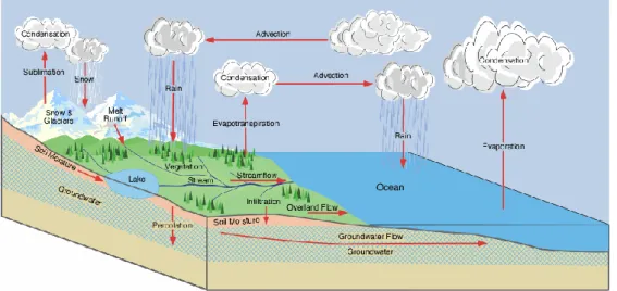
The hydrologic cycle outlines and briefly describes the spatial and physical changes water undergoes annually, as seen in Figure 3. Initially, solar energy with other factors causes the evaporation of water from the oceans and land surfaces. As the water vapour rises to the atmosphere, it condenses into the form of clouds. The clouds travel to another location-driven mainly by wind. As the clouds move to another location where it is a subject to colder atmospheric conditions, the water precipitates in the form of rain, hail, or snow.
Figure 3 Hydrologic cycle (Pidwirny, 2006)
Not all the precipitation becomes runoff; the net precipitation is the remaining precipitation after subtracting the losses due to the evaporation of water from the soil and vegetation, as well as transpiration (known collectively as evapotranspiration). Surface runoff is the fraction of the net precipitation that moves along the surface of a watershed and converges into a stream, which eventually exits the watershed through an outlet. Some of the net precipitation is stored and hindered by surface vegetation by the act of interception, while
11
some infiltrate the soil or percolates into the groundwater. When the precipitation happens in the form of snow or hail, the precipitation that remains frozen is stored in the watershed until it melts to become runoff (Mays, 2005). The hydrological cycle can be represented by the water balance equation that describes the water flow of water into and out of the watershed for a chosen period (as shown in Equation 2).
𝐐𝐬 = 𝐏𝐫 − 𝐄𝐓 − 𝚫𝐒𝐌 − 𝚫𝐆W (2)
Equation 2 water balance equation, where; Pr = precipitation
Qs = surface runoff ET = evapotranspiration ΔSM = the change in soil moisture ΔGW = the change in groundwater storage (Sitterson, et al., 2017)
The runoff is mainly affected by storm and watershed properties. Such properties are storm duration, precipitation amount, intensity soil properties, watershed topography and land cover. Generally, surface runoff is generated due to two cases, saturation excess and infiltration excess. Saturation excess is when the soil is saturated with water, exceeding its water holding capacity. Thus, most of the precipitation runs off to a stream or forms a pond. Infiltration excess is when the precipitation intensity exceeds the infiltration rate of the soil, thus exceeding the rate at which water seeps into the soil causing the excess water to runoff (Sitterson, et al., 2017). Typically, surface runoff is generated by the combination of these two cases. The soil infiltration rate is influenced by the soil moisture content as explained, by the Horton model of potential infiltration capacity, which presents an empirical equation (as shown in Equation 3) for determining the potential infiltration capacity as a function of time (Chin, 2013).
𝒇𝒑 = 𝒇𝒄 + (𝒇𝟎 – 𝒇𝒄)𝒆−𝒌𝒕 (3)
Equation 3 for potential infiltration rate where, fp = potential infiltration rate
fc =minimum infiltration rate
f0 = maximum infiltration rate
12
t = time into the storm (Chin, 2013)
3.2
Linear Regression (statistical model)
Linear regression is a statistical analysis tool that interprets the X, Y variables as independent and dependent variables, respectively. Linear regression formulates an equation showing the relationship between X and Y; if the relationship is assumed to be linear, then it can be represented as,
𝐘 = 𝛃𝟏 + 𝛃𝟐𝐗
Where β1 is the Y-intercept value, and β2 is the slope of the regression line. Furthermore, a statistical model can use linear regression and display the forecasted value as a Y variable using the X variables (also called predictor) as input data. Firstly, the model uses historical data to calibrate itself by formulating equations, that describe the relationship between the dependent variable and independent variables. These equations nearly represent real-time conditions, and thus by adding forecasted X values, a Y value can be calculated (forecasted).
In practice, the regression line will not coincide with all the plotted points; thus, a coefficient of error can be introduced and represented by;
𝒆 = 𝒚 − 𝐲ˆ 𝐘 = 𝛃𝟏 + 𝛃𝟐𝐗 + 𝐞
Where ± yˆ represents over and under predictions, introducing this value helps to fit the regression line to obtain minimal error value (McCuen, 1984). There are several methods for achieving that such as visual fitting, least sum of errors and least sum of absolute errors, but the most common method is the least-squares approach, which would construct a line with the minimised sum of squared errors.
In many cases, a regression model can be dependant on several variables (predictors) rather than just one; this case is called a multiple linear regression model. Consider multiple independent predictors to be X1, X2,...,Xk, where k
13
is the number of independent predictors and those predictors, influence the forecasted value of Y giving the general equation for multiple linear regression model as represented in Equation 4 (Alkarkhi & A.A.Alqaraghuli, 2019).
𝐘 = 𝛃𝟎 + 𝛃𝟏𝐗𝟏 + 𝛃𝟐𝐗𝟐 + ⋯ + 𝛃𝐤𝐗𝐤 + 𝐞 (4)
Equation 4 for the multiple linear regression model
3.3
Nash-Sutcliffe Efficiency Coefficient
The NSEC is a statistical tool that can be used to assess the accuracy of a model by measuring the goodness of fit between computed data and actual data. NSEC gives a value of R2 (can be called the coefficient of determination) as seen in Equation 5.
(5)
Equation 5 the NSEC equation where yi = measured data
ŷi= computed data
ӯi= arithmetic mean of the measured data
The efficiency coefficient is sensitive to significant deviations from the mean value as well as offsets (delay) between computed and measured data; therefore, R2 can describe how reliable a model is. 1 is the ultimate value indicating the computed data curve lies identically on the actual data curve since measured data do not deviate from computed data (Xie, et al., 2019). This coefficient is generally used for evaluating conceptual and linear regression models, of applications in hydrology. A value of 0.5 is considered acceptable, but for an accurate model, a higher value is required. For this report, the NSEC coefficient was used as the primary tool for evaluating a model's accuracy, but in case of significant deviations from the mean value normalised root mean square error (NRMSE) is more reliable in accuracy assessment. The NRMSE measures the average deviation between the measured and computed values and is divided by the arithmetic mean of measured data, in order to present a value unaffected by the units. NRMSE is
14
a measure of error; therefore, a lower value indicates a higher accuracy. For NRMSE, a value of 1 and above represents an unreliable model.
3.4
Aiolos Forecast Studio and The Achelous model
AFS is a forecasting software developed by Vitec AB, AFS creates models based on historical data or even based on old models, to carry out future forecasts of power consumption and power production. The program can import historical forecasts for validation and follow up. The software was named Forecast Studio because it can contain many different forecast models working simultaneously, such as models for hydropower, solar power, wind power, consumption and more. Different sub-models exist within those forecast models, in other words for the same hydropower station, multiple forecasts can be made simultaneously, each with a sub-model having different basin properties. The program was designed to be user friendly with its clear layout, data visualisation techniques and its various facilitative functions for monitoring and forecasting power production (Vitec Energy AB, 2020). The Achelous model focuses on forecasting unregulated hydropower production. Unregulated hydropower means that the power stations lack a dam on the upstream and have little to no storage. Thus, the hydropower production solely depends on the instantaneous access to the water produced by the runoff in the watershed. The Achelous model depends on data from weather stations, historical input and output data, as well as watershed properties to forecast hydropower production rapidly.
There are two components behind Achelous forecasting ability, A hydrological component and a statistical component. The hydrological component contains a conceptual rainfall-runoff model that uses lumped spatial processes to describe the watershed properties. It adopts a slightly different water balance equation than Equation 2 since it includes snow storage computation and unifies groundwater storage and soil moisture storage, as shown in Equation 6.
15
𝑹 = 𝑷𝒓 – 𝜟𝑺 – 𝜟𝑴 – 𝑬 (6)
Equation 6 water balance equation of Achelous model, where R = runoff
Pr = precipitation in the form of rain ΔS = change in storage due to snow cover
ΔM = other change in storage (ground, lakes and groundwater) E = evaporation
While the hydrological component depends on the physical properties of the watershed to forecast the runoff behaviour, the statistical component purely relies on past data to forecast production. It relies on linear regression to forecast power production, as outlined in Equation 7.
𝑷(𝒕) = 𝜶𝑴𝑷𝒕 + 𝜷𝑯(𝒕) + 𝜸 (7)
Equation 7 power production forecasting (statistical component)
Where αMPt = average forecasted production at hour t and βH(t) estimates the sensitivity for differences in the runoff, H is the runoff in mm. The Achelous uses previous production values, for the computations of the statistical part. A reference period (training period) is set for the Achelous to search for similar past intervals, to determine if the power production value will incline or decline (Vitec Energy AB, 2020).
16
3.4.1 Achelous Hydrological Component
Achelous Hydrological Component estimates runoff by firstly calculating the snowmelt, snowmelt is calculated based on the energy budget equations and then added to the precipitation. Secondly, Achelous models the soil storage recharged by the snowmelt and precipitation collectively, where the excess accounts for runoff. AFS developers adopted U.S. Army Corps of Engineers, 1960 as a manual for modelling the snowmelt.
Primarily whenever there is sufficient energy a portion of the snow melts (usually top layer or bottom layer of the snow) and according to the physical properties of the snow, the snow is a porous medium that can hold the snowmelt as liquid water. Whenever the water holding capacity of the snow is exceeded, the snowmelt moves down-gradient to become direct runoff. Also, some might infiltrate the soil depending on the soil properties, moisture content and if the ground surface was frozen or not.
The energy budget equations simulate the snow melting mechanism by relating it to the incident energy sources. Furthermore, those energy sources are both shortwave and long-wave net radiation, convection from the air (sensible energy), vapour condensation (latent energy), conduction from the ground, and the energy contained from rainfall. These energy fluxes are shown in Equation 8 and are labelled Qsn, Qln, Qh, Qe, Qg, and Qp respectively, and all represented as a unit of energy per time per unit area of snow (kJ/m2 per unit of time).
Qm =Qsn +Qln +Qh +Qe +Qg +Qp -ΔQi (8)
Equation 8 energy budget equation where Qm = total energy available for snowmelt Qsn = net shortwave radiation
Qln = net long-wave radiation Qh = convection from the air Qe = vapor condensation energy Qg = energy conduction from the ground Qp = energy contained in rainfall
ΔQi = rate of changein the internal energy stored in the snow
ΔQi represents the energy required to melt the ice in the snowpack, freeze the liquid water in the snow and change the temperature of the snow. Moreover, in
17
warm periods ΔQi represents energy into the snowpack, while in cold periods it represents energy out of the snowpack.
In order to calculate the snowmelt amount a general formula is used as shown in Equation 9; where B is the ratio of heat required to melt a unit weight of snow at 0 °C to that of ice. 334.9 is the value of the latent heat of fusion of water in kJ/kg (energy required to change water from solid-state to a liquid state.
𝑴 = 𝑸𝒎
𝟑𝟑𝟒.𝟗𝝆𝑩 (9)
Equation 9 general formula for calculating the amount of snowmelt where M = snowmelt (mm/time)
Qm = total energy available for snowmelt (kJ) ρ = water mass density (kg/m3)
B = thermal quality of the snow
Usually, the snowpack is composed of snow (ice) with liquid water held within its pores, a snowpack that contains no liquid water would have a thermal quality value of 1, but once melting has begun that value would be less than 1. For a melting snowpack, the thermal quality is usually between 0.95-0.97, that is because the latent heat required to release the water is less than the latent heat of fusion of water.
Radiation energy is the main energy source for earth's surface; some of this energy is solar shortwave radiation and terrestrial long-wave radiation. Shortwave radiation (solar) provides most energy for snowmelt, the net amount of shortwave radiation (Qsn) is the snowpack absorbs that portion of that. The amount of solar radiation reaching the snowpack varies with, altitude, time of day and year, atmosphere, forest cover and reflectivity of the snow (albedo).
The surface of the snowpack reflects a high percentage of the incident solar radiation; at the same time, the snowpack absorbs the rest. Albedo is how much the snow would reflect of the incoming shortwave radiation, for fresh snow albedo is above 80%, and it decreases as the snow get older or refreezes; As seen from Equation 10 of net shortwave energy.
18
𝑸𝒔𝒏 = (𝟏 − 𝑨)𝑰𝒊 (10)
Equation 10 of net shortwave energy available for snowmelt where A=Albedo(expressed as a decimal fraction)
Ii = daily incident solar radiation (kJ/m per day)
The applied equation for calculating the amount of snowmelt from shortwave radiation is acquired by taking Equation 10 and merging it with the general formula of Equation 9 to get Equation 11 with the assumption of thermal quality as 0.97.
𝑴𝒔𝒘 = 𝟎. 𝟎𝟎𝟑𝟎𝟖𝑰𝒊(𝟏 − 𝒂) (11)
Equation 11 amount of snowmelt in mm due to shortwave radiation energy
The earth emits Long-wave radiation (terrestrial) to the outer space in the form of thermal radiation; the atmosphere and forest cover reflect some of this radiation. Snow almost acts as a perfect blackbody for long-wave radiation, where the snowpack absorbs all the incident long-wave radiation. However, snow constantly emits some of the absorbed shortwave radiation back to the atmosphere as long-wave radiation. The net long-wave radiation (Qln) is the difference between the absorbed and emitted long-wave radiation by the snowpack. In clear skies, the absorbed radiation is more than the emitted giving a positive value for Qln, but if the snow was beneath the forest canopy and cloudy sky, Qln might be a negative value. Equation 12 expresses the amount of shortwave radiation that the snow emits.
𝑸𝒍 = 𝟄𝝈𝑻𝒔𝟒 (12)
Equation 12 of emitted shortwave radiation by snow where
Ql = total shortwave energy emitted by the snow (kJ/m2 per second) 𝟄= 0.99 for clean snow
σ = Stefan-Boltzman constant (5.735×10⁻¹¹ kJ/m2 s K4)
Ts4 = blackbody temperature in Kelvin (K)(temperature of the snow surface)
For the computation of black radiation, different factors are included, such as the temperature of the cloud cover, forest canopy, distribution of the water vapour and temperature in the atmosphere. These different factors made it complicated to calculate the snowmelt by long-wave radiation, thus by using
19
experimental data and assumptions, a non-linear relationship between temperature (in Kelvin) and long-wave radiation was produced. This function was reduced into linear relationship through shifting to Fahrenheit temperature scale and by fitting to linear approximations. The final equation for calculating the snowmelt in inches and Fahrenheit is described for two cases;
(a) Snowmelt under clear skies.
𝑴𝒍 = 𝟎. 𝟎𝟐𝟏𝟐(𝑻𝒂− 𝟑𝟐) − 𝟎. 𝟖𝟒 (13)
Equation 13 snowmelt due to long-wave radiation under clear skies
(b) Snowmelt under a forest canopy.
𝑴𝒍 = 𝟎. 𝟎𝟐𝟗(𝑻𝒂− 𝟑𝟐) (14)
Equation 14 snowmelt due to long-wave radiation under a forest canopy
Another source of energy is the turbulent transfer, which is a term used to collectively represent the processes of convection (Qc) and condensation (Qe). The turbulent transfer is of little importance during the spring season where solar energy is dominant. However, during winter, turbulent transfer, along with energy from rainfall, is the dominant energy sources for snowmelt. Convection is the transfer of sensible heat from warm air advected over the snowpack, and the latent heat is provided from the condensation of moisture
from the atmosphere on the snowpack
Equation 15, and
Equation 16 expresses the turbulent transfer.
𝑸𝒄 = 𝑫𝒉𝒖𝒛(𝑻𝒂− 𝑻𝒔) (15)
Equation 15 for energy obtained from convection where Qc = total energy obtained from convection
Dh = bulk transfer coefficient for sensible heat transfer (kJ/m3 °C)
uz =wind speed at a chosen height above the snow surface (m/s)
Ta = temperature at the air surface (°C)
20
𝑸𝒆 = 𝑫𝒆𝒖𝒛(𝒆𝒂− 𝒆𝒔) (16)
Equation 16 for energy obtained from condensation where Qe = total energy obtained from the condensation
De = bulk transfer coefficient for latent heat transfer (kJ/m3 Pa)
uz =wind speed at a chosen height above the snow surface (m/s)
ea = vapour pressure of air surface (Pa)
es = vapour pressure of the snow surface (Pa)
Snow can also melt due to the heat conducted from the ground (Qg), this value is small and usually neglected for short periods, but for long periods and lumped models a value of 0.25-0.76 mm/day is assumed.
Similar to convection from the air, convection from snow by rainfall also accounts as an essential factor in snowmelt. The temperature of the precipitation is assumed to be the same as the air temperature. Melting due to rainfall can be expressed in Equation 17.
𝑸𝒑 = 𝑪𝒑𝝆𝑷𝒓(𝑻𝒓− 𝑻𝒔)/𝟏𝟎𝟎𝟎 (17)
Equation 17 heat convicted by rain where Qp = energy convicted by rain
Cp = specific heat (2.1 kJ/kg for snowfall and 4.2 kJ/kg for rainfall)
ρ = mass density of water (kg/m3)
Pr = precipitation (mm/ unit time) Tr = temperature of rain (°C)
Ts = temperature of snow (°C)
The last energy component in the energy budget equation is the internal energy of the snow. When the heat deficit of the snowpack is positive (snowpack's temperature below freezing), that deficit can be decreased when rain and meltwater freeze inside the snowpack. This phenomenon will stop when the snowpack temperature reaches 0°C, where the snowpack will become isothermal. The internal temperature is expressed in Equation 18, i,l and v stand for ice, liquid and vapour, respectively, but the vapour component is negligible.
21
𝑸𝒊 = 𝒅𝒔(𝝆𝒊𝑪𝒑𝒊+ 𝝆𝒍𝑪𝒑𝒍+ 𝝆𝒗𝑪𝒑𝒗)𝑻𝒎 (18)
Equation 18 internal energy of the snow where Qi = internal energy of snow
Cp = specific heat (2.1 kJ/kg for snow and 4.2 kJ/kg for water)
ρ = mass density (1000 kg/m3for water and 922 kg/m3for ice)
3.4.2 Achelous basin properties
Each power station can have its basin properties, and those properties simulate the physical parameters of a watershed. The basin properties include forest canopy, altitude, max storage (field capacity), discharge rate per hour, delay, snow depth and minimum standard deviation of runoff, as shown in Figure 4.
Figure 4 basin properties window in AFS
The forest canopy field represents the portion of the watershed that the model considers as forest; it has a significant effect on the snowmelt calculations and is represented by a fraction from 0-1.
The snow depth field represents the amount of snowpack (in mm) present at the training period start, and this is an optional setting used in recalibrating the Achelous models. When the snowmelt contribution to the runoff is overestimated or underestimated, this setting can be used to recalibrate the model.
The minimum standard deviation field specifies the minimum permitted value for the standard deviation of a parameter involved in the regression. If any parameter has a lower standard deviation than the set value (in mm), no regression will take place, and the model will rely on the statistical component and real-time correction instead.
22
The max storage field represents the average storage capacity of the watershed soil (in mm) when the storage capacity is exceeded all the precipitation accounts for runoff.
The discharge rate represents how much of the stored amount of water in the soil escapes the groundwater (per hour) and flows back to the stream to contributes to power production. Both the max storage and the discharge rate field enables the smoothening and reduction of the runoff curve, to better simulate the actual runoff phenomena. The runoff curve peaks can be too high if the max storage was set to a low value, or the discharge rate was too high (Vitec Energy AB, 2020).
3.4.3 Achelous statistical component
The statistical component is the main driver of the Achelous model since it cannot be disabled; the statistical component uses stepwise regression analysis with multi variables (predictors). The statistical component has two functions: it relates the runoff to the power production and estimates the delay between the runoff and production. The delay is determined by the distance between the weather observation station and the power station, topography, nature of the ground, systematic errors in the weather forecasts.
Generally, the statistical part assumes the production at time t similar to a historical time with similar conditions; moreover, it adopts the interval directly preceding the forecast time for comparison, where the model uses predictors to search the historical production for similar intervals. The model selects those intervals based on the predictors of power production and runoff directly. At the same time, the cloud cover, precipitation, air pressure, relative humidity and temperature serve as indirect predictors since they influence the runoff. The statistical component uses Equation 7 for forecasting production; the value of average forecasted production (αMPt) is estimated using the intervals. Furthermore, the model searches for sensitivity difference in runoff (βH(t)), which is the impact of runoff difference between the preceding period and forecasted period. The impact can be an increase in production, a decrease in production or no change. The impact is taken as both instantaneously and retrospectively, then calculated by creating secondary predictors of the inflow. The secondary predictors include the runoff, the runoff delayed by 1 and 2
23
hours, the average runoff 6, 12, 24 and 48 hours, and All these are expressed as deviations from the corresponding averaged values.
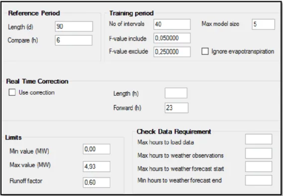
The statistical component performance depends on the training period of the model, which can be tuned from the reference and training period parameters, as seen in Figure 5.
Figure 5 Statistical component parameters
The reference period specifies the number of days in historical production used for the search, where the model searches for similar intervals, moreover the No of intervals parameter controls the number of the similar intervals the model chooses. The Compare parameter determines the length of the interval directly preceding the forecast period, that will be used for the search of similar past intervals of the same length. For example; if a reference period were set to 90 days with an interval period of 12 hours and 30 intervals, the model would look
24
for 30 best matching intervals searched for 12 hours within those nine days. The intervals are furtherly divided into hourly sub-intervals, so it can be said that the compare parameter indirectly determines the number of subintervals. F-value include in a stepwise forward regression model, the model starts as empty without predictors, for determining the predictors to be included in the model, a statistical test based on the partial correlation coefficient for each predictor is used. F-value include specifies the significance level for an error that a model a shall include, and the value will act as a probability of including an uncorrelated predictor and is used as a stopping criterion for the stepwise regression. As the model runs for each step of the procedure, if the model cannot find a significant predictor, the maximum number is set, and the last predictor with the least significant value is excluded. If the F-value include is set to 0.05, that means the model will risk including an uncorrelated predictor having an error in 5% of the cases taken.
F-value exclude as the model runs, for each step of the stepwise procedure; it makes a backward check to determine if any of the already included predictors should be now excluded. The program carries out a partial F test based on the partial sum of squares (SS) for each of the predictors which are included in the model, then exclude the predictor with the highest probability to fall short of the significance value set in the F-value exclude box. In summary, this parameter enables the user to set the risk of keeping a predictor that was relatively significant in the previous step but no longer in the current step. To acquire a conservative model that generally does not throw out variables, that have already been included, the value of F-value exclude should be more than the F-value include.
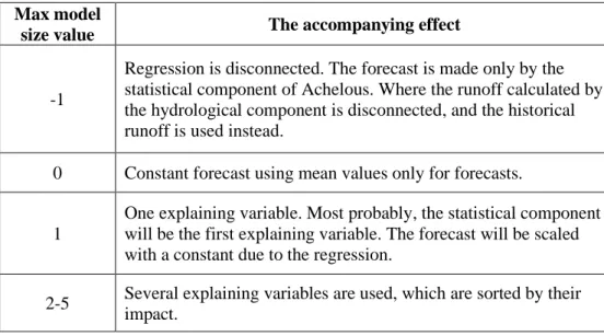
The predictors to be used in the statistical component can further be controlled by changing the max model size value, as shown in
25 Table 1.
26
Table 1 Effects of different Max model size values Max model
size value The accompanying effect
-1
Regression is disconnected. The forecast is made only by the statistical component of Achelous. Where the runoff calculated by the hydrological component is disconnected, and the historical runoff is used instead.
0 Constant forecast using mean values only for forecasts.
1
One explaining variable. Most probably, the statistical component will be the first explaining variable. The forecast will be scaled with a constant due to the regression.
2-5 Several explaining variables are used, which are sorted by their impact.
To relate what the runoff in mm equates to in production, a parameter of runoff factor (r) is set, which mainly bridges the hydrological component of Achelous with the statistical component. The runoff factor ranges from 0-1, where 0 means none of the runoff contributes to production, and one means that all of the runoff contributes to production. A possible misconception is that the runoff factor parameter explains how much of the physical runoff enters the turbine, which would be true in a physically-based model using Equation 1, but that is not the case here since the Achelous is a statistical model. The r parameter indicates how dependent the statistical component is on the runoff as a predictor; Equation 19 computes the total MAE for the sub-intervals, on which the degree of similarity to the interval preceding the forecast period is evaluated.
27
𝐌𝐀𝐄 = (𝟏 − 𝐫)𝐌𝐀𝐄𝐩+ 𝐫(
𝐌𝐏
𝐌𝐑)𝐌𝐀𝐄𝐫 (19)
Equation 19 Mean absolute error for the sub-intervals where r = runoff factor
MAE = mean absolute error
MAEp = mean absolute error in production
MP = mean production MR = mean runoff
MAEr = mean absolute error in runoff
The total MAE of a sub-interval is calculated by; dividing the mean production of the training period to its mean runoff (to provide a rough estimate of how runoff in mm equates to production)—then multiplied by runoff and the MAE of the runoff, to give weight to the influence of the runoff. Second, the influence that MAE of production is weighted by multiplying it with 1-r; this explains the influence of the other predictors.
The sub-intervals are disabled for forecast periods with monotonically non-increasing inflow if they are followed by periods where the largest absolute difference between two values corresponds to an increase in production. This condition prevents inaccurate runoff values to have an undesirable effect on the forecast accuracy.
28
3.4.4 Aiolos Forecast Studio built-in evaluation tools.
AFS forecast studios evaluate its production forecasting using mean error (ME), mean absolute error (MAE), and root mean square error (RMSE). These tools actively evaluate the power forecast made by AFS but do not evaluate the accuracy of the hydrological component in the Achelous. Thus, to assess and inspect the model accuracy, the runoff model will be evaluated separately using Microsoft Excel.
(20)
(21)
(22)
Equation 20, 21, 22 for Aiolos built-in evaluation tools where yi = measured data
fi= computed data
n= No. of values e= error
RMSE like the NSEC is a good tool to evaluate a model's accuracy. However, it has an advantage over the NSEC with its suitability to evaluate non-linear models (Zhong & Dutta, 2015), but RMSE has a variable range of values depending on the models unit. Moreover, if the model output values were large, the RMSE value would be large as well.
29
3.5
ArcMap (GIS)
The geographical information system (GIS) is a powerful tool for facilitating the management and analysis of geographical or spatial data.
ArcMap is a GIS computer software developed by Esri, designed to serve many purposes and has a comprehensive and various range of applications. Of which most relative to this study is; its ability to create maps, perform analysis and manage geographical data. This software has an informative and easy to use user interface where it represents the data in layers and tables, with the option of exporting those in the format of other commonly used computer programs. ArcMap contains numerous geoprocessing tools that drive its applications; these tools deal with data in the form of tables, vector and raster layers. The vector layers compose points, lines and polygons, where these layers are accompanied by an attribute table that sorts these components into rows and permits the addition of properties to each component in columns. These properties can be area, volume, name, type and more. ArcMap tools also provide the means for performing calculations, transformations and analysis to the attribute table for acquiring more data. Raster layers represent the data in a grid of cells, and each cell can represent one unique type of data, in this study raster layers are used to represent the elevation and land use of a watershed. ArcMap can be used to compensate for the lack of AFS in visually presenting some data helpful to the understanding of the physical properties of a watershed. Moreover, it can be used in the computation of the physically-based parameters of the AFS models; necessary for the model calibration. (esri, 2020)
30
4
Delimitations, limitations and Assumptions
Primarily certain delimitations were set to this study to serve as boundaries for this report's scope of work. Firstly this study revolves around improving the RORs production forecasting, thus is not applicable for large dams or hydropower stations of considerable water storage capacity in their upstream. Secondly, Småkraft's run of river hydropower stations in Norway was adopted as a case study for the availability of needed data and resources. Fortum manages the production forecasts for Småkraft and AFS was chosen as a tool for the forecasting production of those RORs since it is implemented in other processes at Fortum. Finally, Achelous hydrological model was constructed to simulate the actual runoff in Norway and regions of similar topographical properties.
During this study, certain limits were encountered, that prevented the forecast accuracy from being increased further. Those limits are;
a) error percentage in the weather forecasts since the Achelous relies on weather forecast data for forecasting power production and runoff, and error in the input data limits the accuracy of the model.
b) the use of empirical relationship by the Achelous to describe the direct runoff, this relationship enables the user to adjust the runoff curve to fit the historical runoff better. However, it fails to simulate peak flows, runoff during wet periods and snowmelt.
c) while inspecting the historical data given by AFS, some missing or faulty historical production data were encountered. Historical production data has a considerable influence on Achelous ability to forecast power production; therefore, limitation impacts the accuracy of the forecasts.
d) unavailability of actual historical runoff values in AFS, where the historical runoff is substituted by the runoff calculated with the latest weather forecasts. Some assumptions were made in the making of this report, first of which is that the historical runoff values created by AFS are reliable and thus were used in evaluating the accuracy of the runoff forecasts. Secondly, the application of the lumped model assumption, in order to acquire certain parameters. The final assumption was that this model provides hourly forecasts making the forecast curve more detailed thus accuracy of 50% is acceptable, whereas, in daily mean models, higher accuracies are preferred.
31
5
Preliminary Model Accuracy Assessment
Vitec has already set the hydropower model parameters values for each power station; therefore, it is necessary to evaluate the current model and use the evaluation results as a benchmark for future comparisons. The Achelous forecasts power production using two components statistical and hydrological, working together to increase the accuracy of the forecasts. In a meeting with Vitec developers, they stated that it is possible to disable the hydrological model, but not the statistical model. Also, the model automatically disregards the hydrological model forecasts if they increased the error percentage.
5.1
Input data
AFS is a server-based program that gets a live feed of weather data from local providers, which is used for production forecasting; the weather data includes temperature, precipitation, cloud cover and relative humidity. It also stores recorded actual data and forecast results; thus, these data will be used for assessing the model accuracy. Fortum has been running AFS for its RORs since late December 2019, which is a short period for running evaluations. Luckily, AFS contains the 'follow up' tab which enables the back-casting feature. Through this feature, AFS can access historical weather and hydrological data of a period even before its installation. With those historical data, the follow-up function can back-cast power production and runoff, then plotting it along with measured values.
5.2
Procedure and Results
The assessment procedure starts with carrying out back-casts between the period of 1/1/2019-1/1/2020 (a whole year); naturally better observations can be made by looking back-casting for a longer period than a year, but currently, such data is not available. The back-casting was done for the hydropower stations of Holmen and Jordalen 2 using AFS follow-up tab. The follow-up function uses the model's current parameter values to simulate the production forecasts in the past with the given historical weather data. The first step was to choose the type of extract, which defines the values to be chosen from the forecast for comparison with the actual values. The recreated extract is chosen so that the model recreates forecasts as it would have been in the past. After
32
the forecasts were calculated, they were exported to excel sheet to be used for evaluation. The exported data included measured and forecasted values for load and runoff, where the hydrological component calculates the runoff values. The evaluation results of power production forecasts are seen in Table 2.
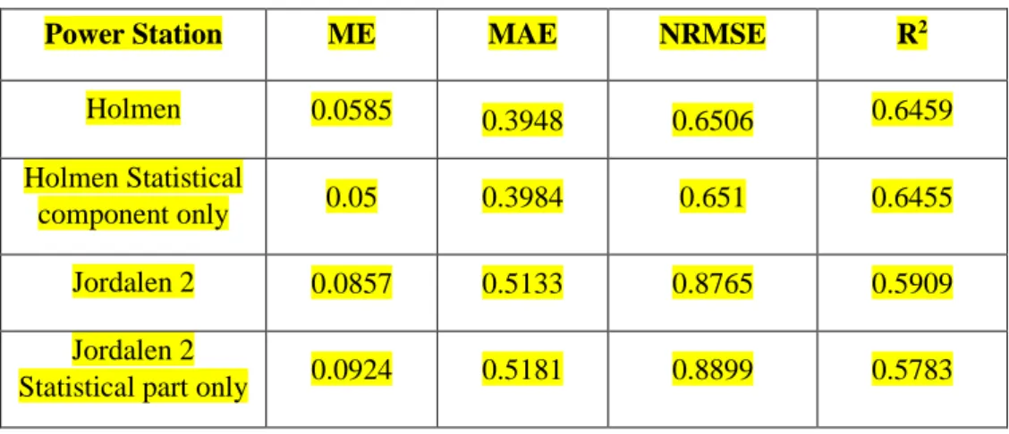
Table 2 Evaluation results of power production forecasts
Power Station ME MAE NRMSE R2
Holmen 0.0585 0.3948 0.6506 0.6459
Holmen Statistical
component only 0.05 0.3984 0.651 0.6455
Jordalen 2 0.0857 0.5133 0.8765 0.5909
Jordalen 2
Statistical part only 0.0924 0.5181 0.8899 0.5783
First back-casts done returned R2 values of 0.64 and 0.59 for Holmen and Jordalen 2, respectively. This value is above 0.50, which makes it acceptable but not considered highly accurate, leading to the next step of investigating the cause of this low value. As mentioned earlier, Achelous relies on two components for forecasting power production; therefore, it was crucial to investigate the performance of these two components. The investigation began by disabling the hydrological model; this was done by setting the max model size to (-1). It can be seen from Table 2 that the hydrological model barely increased the accuracy of the model, leading to the next step of evaluating the hydrological model accuracy. It is not possible to disable the statistical component of Achelous as was done for the hydrological component, thus by inspecting
33
Equation 6, Equation 7 and Aiolos user manual, it can be understood that the runoff is forecasted solely from the hydrological component. R2 was calculated for the runoff, as shown in Table 3. The accuracy of the runoff forecast is very poor; for Holmen, it was a negative value indicating that the model performance is unacceptable. This poor accuracy can be caused by incorrect calibration or wrong understanding of the watershed properties.
Table 3 Evaluation results of the runoff forecasts
Power station R2
Holmen -0.0927
Jordalen 2 0.0365
In conclusion, the current accuracy is given by the statistical component only, because the hydrological component is disregarded, due to giving out poor results. The next step would be to optimise the production forecast accuracy by improving the hydrological component. Correspondingly the optimisation shall comprise adjusting the model parameters to improve the simulation of the water behaviour in the watershed; given that the hydrological component is based on sound theory and can estimate hourly runoff values. Recalibration of the model will involve extracting values for adjusting the watershed properties to simulate the runoff phenomena better. ArcMap (GIS) computer program will be used to extract those values by importing reliable layers of those watersheds, on which suitable tools (from ArcMap) will be used for computation and analysis.
34
6
Recalibration
Before this study, Fortum calibrated the models for each of its RORs and are currently using them for their power production forecasts; this study aims to increase the accuracy of these models even further. Recalibration of these models is necessary and shall follow a systematic approach applicable to all the models, and that requires a wholesome understanding of the Achelous model.
The recalibration underwent several phases that involved literature reading, model trials and meetings with AFS developers. This study had several hypotheses regarding improving the accuracy, some proved to work, others failed or were inapplicable, but the outcome was a guideline on improving the forecast accuracy by adjusting the value of the parameter.
The first step of the recalibration involved adjusting the basin properties of the models to simulate the runoff phenomena better, and this was done with the help of ArcMap (GIS). Some parameters, such as forest canopy, max storage, altitude, and delay, were planned to be calculated with the help of GIS. The reason for adjusting the hydrological component first is to evaluate its effect on the total model accuracy.
The second step was to adjust the statistical component parameters by understanding the relation to the hydrological component and the effect of different predictors accuracy. The excel sheet used for the accuracy assessment has proved to be a powerful tool for recalibrating the statistical component since Aiolos built-in accuracy assessment tools are limited to the power production only.
The final step was to validate the procedure by applying the approach to other hydropower stations and use the excel sheet to assess and compare the results. As mentioned earlier, the Achelous model only assesses the accuracy of the power production forecasts, which is not enough to make the necessary observations to be adopted by this study.
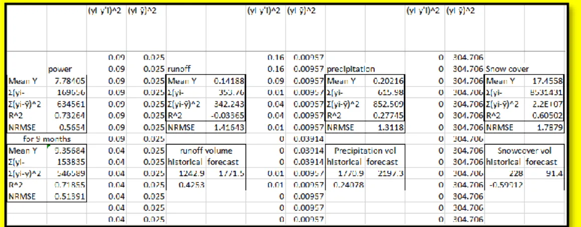
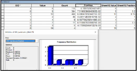
A large part of this study's scope included the formulation of an excel sheet specialised in analysing the output data from the model; statistical analysis accompanied every step of the recalibration procedure as well as investigating the Achelous model performance. Measured and forecasted values of production, runoff, precipitation and snow cover are extracted from AFS and
35
imported into the excel sheet, where these data are compared and analysed using NSEC, NRMSE and Volume difference as shown in Figure 6.
Figure 6 a sample of the excel sheet
The excel sheet was used to inspect the influence of the changes made on the model parameters, during every step of the recalibration to ensure higher forecast accuracy. Also, by inspecting the influence of these parameters on the forecasts provided a better understanding of the model parameters and how to adjust the forecasted curve to fit the actual curve better. The excel sheet includes two spreadsheets for each hydropower station; one which evaluates the standard model and the second for the recalibrated model for comparison.
36
6.1
Improving the runoff forecast accuracy
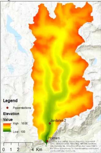
Determining the basin properties using GIS included using both vector and raster layers taken from reliable sources, in addition to creating points and other layers.
The procedure started by setting up the environment for the map, the layers are saved in geodatabase file and choosing the projected coordinate system of ETRS 1989 ETRS-TM33 since it is the adopted geographical reference system in Norway.
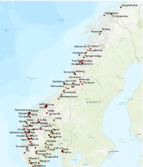
The first layer added was the world map stored as a Basemap in the ArcMap program, then a vector layer was made representing the power stations located on the map each power station represented as points as seen in Figure 7. The power stations layer was created from data provided by Fortum, which included names, coordinates, elevation, power production capacity and other information of each power station. From Figure 7 it can be seen that the RORs are widely distributed over Norway, next step was identifying the watersheds in Norway, in which vector layers for watersheds and streams were taken from (NVE, 2019). After carefully inspecting the streams, watersheds, and power stations layers two RORs Holmen and Jordalen 2 were chosen for calibration since they have a respectively high amount of power production and lie in the same watershed. Importing layers for all of Norway would make the file size too large and in turn significantly slow down the program. Therefore, most layers were cropped by selecting the needed data and exporting it as a new layer or by downloading layers for the region of the concerned watershed and not all of Norway if available.
37