O R I G I N A L R E S E A R C H
Open Access
Parallel computing of multi-contingency
optimal power flow with transient stability
constraints
Yude Yang
1*, Anjun Song
1, Hui Liu
1, Zhijun Qin
1, Jun Deng
2and Junjian Qi
3Abstract
To deal with the high dimensionality and computational density of the Optimal Power Flow model with Transient Stability Constraints (OTS), a credible criterion to determine transient stability is proposed based on swing curves of generator rotor and the characteristics of transient stability. With this method, the swing curves of all generator rotors will be independent one another. Therefore, when a parallel computing approach based on the MATLAB parallel toolbox is used to handle multi-contingency cases, the calculation speed is improved significantly. Finally, numerical simulations on three test systems including the NE-39 system, the IEEE 300-bus system, and 703-bus systems, show the effectiveness of the proposed method in reducing the computing time of OTS calculation.
Keywords:Power system, Transient stability, Multi-contingency, Optimal power flow, Parallel computing
1 Introduction
With the development of smart grid, the operation of power system is close to its stability limit state fre-quently. In the event of a contingency or a large disturb-ance, large-scale blackouts or even the whole system crashes would happen. However, Optimal Power Flow with Transient Stability Constraints (OTS) can integrate the economic and dynamic security of the system into the same framework, which has become an effective tool to get the safety of the system.
Lots of research work has been devoted to the classical OPF [1–4]. However, OTS has become a challenge from the model description to the design of algorithms [5, 6], due to the transient stability constraints of ordinary dif-ferential equations. In [7], the ordinary differential equa-tions are differentiated into algebraic equaequa-tions, while the transient stability constraints are discretized into in-equality constraints. As a result, the OTS problem is solved by the conventional optimization method, but the number of variables and equations are increased signifi-cantly, resulting in long computation time and difficult convergence. However, references [5,8] are two classical
articles dealing with OTS problems practically. The the-oretical development in [5] is that dynamic equations are converted to numerically equivalent algebraic equa-tions. And in [8], OTS gets the same size of the OPF problem by an equivalent transformation from differen-tial equation constraints to the inidifferen-tial value constraints.
However, in the Jacobian matrix of OTS, a large num-ber of dynamic sensitivity equations must be dealt with in each iteration of the optimization process [9]. The dy-namic sensitivity equation which describes the dydy-namics of power systems is a set of differential algebraic equa-tions (DAE) with the same size and can only be solved by numerical integral methods with massive calculation.
The work of this paper is based on [8, 9], where a credible criterion is proposed based on swing curves of generator rotor and the characteristics of transient sta-bility. High-performance science and engineering com-puting [10], represented by parallel technology, has become an important approach of increasing productiv-ity in various industries [11–14]. By using MATLAB par-allel computing toolbox, the OTS problem is solved within reasonable computing resources with the com-puting speed reaching to the practical or even online level [15, 16] compared with the existing methods proposed in [17–19].
* Correspondence:[email protected]
1Guangxi Key Laboratory of Power System Optimization and Energy
Technology, Guangxi University, Nanning, China
Full list of author information is available at the end of the article
Where PGi refers to the active power output of ith power source;SGis active power sources set;Snis the set of all nodes;PDi is the active power load of ith power source.
2) Equality constraints.
There are two parts in this section, including power flow equations and swing equations of generator.
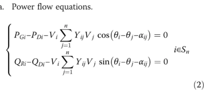
a. Power flow equations.
PGi−PDi−Vi
Xn
j¼1
YijVj cos θi−θj−αij
¼0
QRi−QDi−Vi
Xn
j¼1
YijVjsin θi−θj−αij
¼0 8
> > > > < > > > > :
i∈Sn
ð2Þ
Where QRi refers to the reactive power output of ith power source;QDi is reactive power load at busi; Vi, θi are the magnitude and phase of voltage at bus i separ-ately; Yij, αijare magnitude and phase of transfer admit-tance between busesi,j.
b. Swing equations of generator.
Pei¼Ei j∈SG
Ej Geijcos δi−δj
þBeij sin δi−δj
ð4Þ
3) Inequality constraints. a. Operating constraints:
f
PGi≤PGi≤PGi i∈SGQRi≤QRi≤QRi i∈SR
Vi≤Vi≤Vi i∈Sn
Pij≤Pij≤Pij i∈SCL ð5Þ
Where PGi;PGi, QRi;QRi are upper bound and lower
bound of active and reactive power sources;Vi;Vi,Pij;P
ij are upper bound and lower bound of voltage
magni-tude at busiand power flow at lineij;SR,SCLare react-ive power sources set and lines set.
b. Stability constraints:
Stability criteria are as follows:
δ≤δi−δCOI≤δ ð6Þ
Fig. 1Explanation of conventional transient stability constraints. Whether the system transient stability requirement is satisfied or not can be determined by calculating whether the sum of the excess area of each generator’s swing curve is less than or equal to zero
Where δ;δ upper bound and lower bound of rotor relative swing are angle; δCOI is inertia center angle, which is defined as follows:
δCOI ¼
Xng
i¼1 Miδei=
Xng
i¼1
Mi ð7Þ
Where Mi stands for the moment of inertia of theith generator.
2.2 Transient stability constraints
The transient process of power system is described by differential algebraic equations. The related transient sta-bility preventive control problem is an optimization problem with differential algebraic equations. Its general form can be described as follows:
minF x0ð Þ ð8Þ
s:t:h x0ð Þ ¼0 ð9Þ
g≤g x0ð Þ≤g ð10Þ
_
xkt ¼ Fk xkt ;xk0¼x0 ð11Þ
hk xkt ¼0 ð12Þ
gk xkt ≤0 ð13Þ
Formula (8) is the objective function. Formula (9) is a power flow equation. And formula (10) represents static security constraints, including the voltage limit, gener-ator output limit, etc. Formula (11,12) represent transi-ent stability equality constraints. And formula (13) represents the transient stability inequality constraints under each contingency.
In this paper, based on the functional transformation technique, transient stability constraints (11–13) formu-las are converted into a unique inequality equation.
The traditional time-domain simulation of transient stability analysis considers that the rotor of the unit and the center of inertia relative swing angle does not exceed a given limit angle, which can be considered the system run synchronously without loss of stability in the rolling process.
The formula is as follows:
gið Þ ¼t jδið Þt −δCOIð Þt j−δmax≤0; i∈SG ð14Þ
Whether the system transient stability requirement is satisfied or not can be determined by calculating whether the sum of the excess area of each generator’s swing curve is less than or equal to zero.
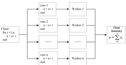
Fig. 3Cycle decomposition diagram. That is, the parallel loops can be decomposed and processed by client and worker modes. Client refers to a CPU kernel that performs and assignments parallel tasks. Worker refers to the other CPU cores that run parallel code, and all workers work at the same time to achieve accelerated computing
Table 1Summary of the three test cases
Cases Number of
Generators/ Buses/Lines
Objective Function of Conventional OPF
Iterations of Conventional OPF
Computation Time(s)
NE39 10/39/34 61.8135 12 0.04
IEEE300 69/300/304 233.6095 17 0.28
C703 99/703/800 130.5660 18 0.57
Table 2Test results of NE-39 system
Contingency Line
Integration Step(s)
Iterations Objective Function
Computation Time(s)
Branch 8–9 0.01 12 61.8135 0.26
0.02 11 61.8131 0.14
Branch 21–22 0.01 18 61.8208 1.16
Si¼
ZT
0
hið Þx dx≤0;i∈SG ð15Þ
And the formula (11–13) is transformed into formula (15). However, when formula (15) is added as an in-equality constraint, the convergence is not satisfactory with low computational efficiency.
Therefore, based on the contents of Fig. 1, this paper presents a simple and effective method to determine the transient stability of the system under the given power angel limit.
In the relative swing curve of all generator rotors, there must be at least one point deviated from the high-est point. If the point satisfies formula (14), the transient stability condition of the system can be considered to be satisfied. As is shown in Fig.2.
Thetmpoint of the generator 1 represents the highest point that deviates from the center of inertia in all the generators. Once the generator 1 is constrained, the other generators, including the generator 2 and the gen-erator 3, naturally satisfy the constraint conditions.
Assuming that the point is thetmtime of theith gener-ator, the constraint expression can be obtained:
gið Þ ¼tm jδið Þtm −δCOIð Þtm j−δmax≤0 ð16Þ
Formula (16) can be used as the transient stability in-equality constraint instead of the formula (14). The model after conversion is as follo6ws:
minF x0ð Þ ð17Þ
h x0ð Þ ¼0 ð18Þ
Jacobi and Hessian array of formula (20) can be obtained as follows:
∂gtm
∂x0 ¼
∂gtm
∂xtm
∂xtm
∂x0
∂2g
tm
∂x02 ¼
∂2g
tm
∂xtm2
∂xtm
∂x0
∂xtm
∂x0 þ
∂gtm
∂xtm
∂2x
tm
∂x02 8 > > < > > : ð 21Þ
Where gtm is an explicit expression for xtm, so ∂gtm=∂ xtm and∂
2 gtm=∂xtm
2 can be derived directly. Whilex
tm is
not an explicit expression for x0, ∂xtm=∂x0 and ∂ 2x
tm=∂ x02can be calculated as follows:
d dtm
∂xtm
∂x0
¼∂∂F xtm
∂xtm
∂x0 þ
∂F
∂x0 d
dtm
∂2x
tm
∂x02
¼∂∂2F xtm2
∂xtm
∂x0
∂xtm
∂x0 þ
∂F
∂xtm
∂2x
tm
∂x02 þ
∂2F
∂x02 8 > > < > > :
ð22Þ
Formula (21) can be solved by any method that can ef-fectively solve differential equations and the fourth-order Runge-Kutta method is used in this paper. According to the formula (21–22), for each contingency, the swing curve of all the generator rotors can be calculated separ-ately without affecting each other.
In solving the multi-contingency problem, each con-tingency requires repeated calculations, which is the most time-consuming place as well. As the size of the system expands, the time in this place even occupies more than 90% of the total computing time. Therefore, aiming at the main time-consuming part of the program, a parallel algorithm is designed in this paper to allocate the tasks according to the expected multi-contingency.
A diagram for the proposed approach is shown in Fig. 3. That is, the parallel loops can be decomposed and processed by client and worker modes. Client re-fers to a CPU kernel that performs and assignments parallel tasks. Worker refers to the other CPU cores that run parallel code, and all workers work at the same time to achieve accelerated computing.
The parallel architecture of this paper relies on MATLAB parallel computing toolbox. The key method
Table 4Test results of C-703 system
Contingency Line Integration Step(s) Iterations Objective Function Computation Time(s)
Branch 10–442 0.01 49 130.5784 32.6
0.02 51 130.5781 13.13
Branch 681–337 0.01 18 130.5660 1.9
is running parallel for-loops on workers within contingencies.
And there are three main variables which should be classified before the parallel for-loops.
1) Loop Index Variable
The loop variable represents the number of times the loop is executed. The parallel strategy in this paper is used in the expected multi-contingency.
2) Sliced Variable
The large variable array contains all contingencies can be segmented into each worker by using sliced variable in the implementation of the parallel for-loops program
i and therefore the data transmission between worker and client is reduced. The array contains all the contin-gency information is actually a contincontin-gency variable in this paper.
3) Broadcast Variable.
Data arrays contains nodal admittance matrix, gener-ator operating data and parameters are classified as
broadcast variable which will be shared by all the workers.
Multi-contingency OTS problem parallel computing process is as follows:
1) First of all, the conventional optimal power flow calculation is carried out without considering the transient stability constraints of formula (20), only the calculation of formula (17–19) are solved. Then taking the optimal solution of the conventional optimal power flow as the initial value, the transient stability analysis is carried out to determine
whether the formula (20) is satisfied. If the optimal solution is satisfied, the calculation is terminated; otherwise, the next step is taken.
2) The initial values of the parameters under each contingency are passed to each worker, and each worker calculates the Jacobian and Hessian matrix independently to complete the iterative calculation of the interior point method.
3) In the iteration process, it’s necessary to judge repeatedly whether the solution of formula (20) and formula (17–19) are satisfied. If both satisfied, the calculation is terminated; otherwise, the calculation process above is repeated.
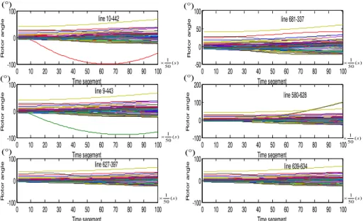
Fig. 4Swing curves in line 21–22 contingency of NE-39 system
4 Numerical results 4.1 Test systems summary
In this section, the NE-39 system, the IEEE 300-bus sys-tem and 703-bus syssys-tems are used for simulation from the aspects including computing time, speed-up and effi-ciency. Furthermore, the simulations are run on 32 Cores 1.8 GHz with 16 GB of RAM. Set the simulation timeT= 2s, the integral step sizeΔt= 0.01s or0.02s, and the swing angle limit is ±100°. A numerical summary of the three systems is listed in Table1.
4.2 Simulation analysis of single contingency OTS
Formula (16) is used as transient stability constraint to solve the OTS model (17–20). Test results of three sys-tem are shown in Tables2,3and4.
From Table1to Table4, the calculation results of con-tingency lines of branch 8–9 in NE-39 system, branch 5–1 in IEEE-300 system and branch 681–337 in C-703 system including the objective function and iterations is completely consistent with the conventional OPF calcu-lation, which shows that the swing curve can meet the condition of angel limit ±100° under the transient stabil-ity analysis without adjustment when the conventional optimal power flow result is used as the initial value, also called‘inactive contingency’.
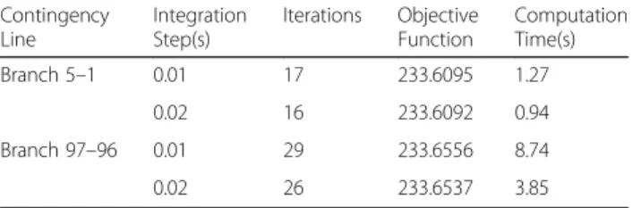
In the meantime, the calculation results of contingency lines of branch 21–22 in NE-39 system, branch 97–96 in IEEE-300 system and branch 10–442 in C-703 system
has a larger objective function and more iterations com-pared with the conventional OPF calculation, indicating that the swing angle of generators reaches the upper limit when expected contingency are calculated, which means that the contingency must be unstable without constraints, also called ‘active contingency’. In order to meet the requirements of transient stability, economy is sacrificed properly, and more iteration is added to adjust the system operation mode meanwhile.
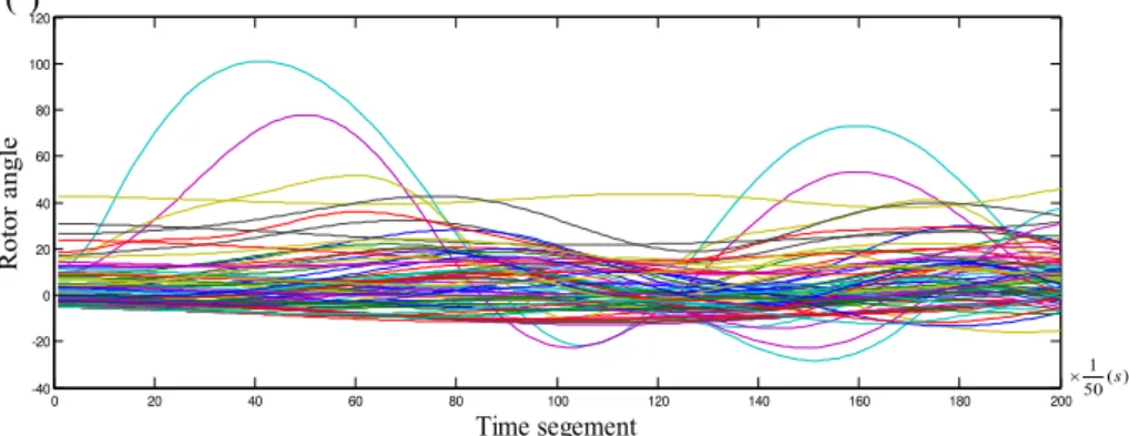
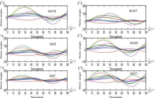
The swing curves of three test systems are shown in Figs.4,5and6.
4.3 Simulation analysis of multi-contingency OTS
Test results of three systems are shown in Tables 5, 6 and7.
From Table 5 to Table 7, iterations of the NE-39 system and the IEEE-300 system changes from 17 to 55 and from 26 to 56 respectively and iterations of the C-703 system changes little when considering multi-contingency. In particular, with the same num-ber of iterations, the calculation time increases ap-proximate linearly as the number of contingency increases, reflecting the good computational charac-teristics of the model in this paper.
According to the results of C-703 system, when considering three contingency, the results of object-ive function is consistent with the results of the first
Fig. 6Swing curves in line 10–442 contingency of C-703 system
Table 5Test results of NE-39 system under step 0.02 s
Number of Contingencies
Iterations Objective
Function
Computation Time(s)
2 23 61.8367 1.11
3 27 61.8526 1.47
4 40 61.8525 1.91
5 38 61.8529 2.35
6 55 61.8529 2.61
Table 6Test results of IEEE-300 system under step 0.02 s
Number of Contingencies
Iterations Objective
Function
Computation Time(s)
2 26 233.6813 7.2
3 26 233.7066 9.78
4 40 233.7571 13.27
5 40 233.7573 17.46
contingency which shows that the first contingency plays a dominant position when considering the pre-vious three contingency. The system adjustment mainly aims to the constraints of the first contin-gency which can meet the constraints of other con-tingency as well. However, when considering 6 contingency, the 4th contingency becomes the dom-inant contingency. Therefore, if the leading contin-gency in the sets can be found, a great amount of computation of OTS problem can be reduced effect-ively, which can be another research goal in the future.
The swing curves of three test systems are shown in Figs.7,8and9.
4.4 Simulation analysis of parallel computing
4.4.1 Performance index
Speed-up refers to the ratio of computation time that the same task running on a single-processor and parallel pro-cessor system, which is used to measure the performance
of parallel programs. In the field of parallel computing, the speed-up ratio is defined as
Sp¼
Ts
Tp ð
23Þ
Where Ts and Tp refers to the serial execution time and parallel execution time, respectively.
Speed-up can reflect the overall performance of the program, but can’t describe the role of each processor, so the concept of parallel efficiency is proposed:
Ep ¼
Sp
q ð24Þ
q is the core number involved in the calculation,Spis the speed-up ratio mentioned above.
4.4.2 Results and analysis
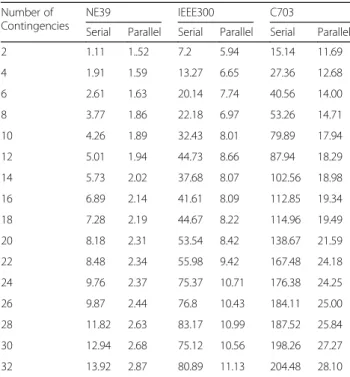
Benchmark results are shown in Table8. Speed-up ratio and parallel efficiency are shown in Table9.
For all the test systems, it’s found that the speed-up ra-tio increase with the number of contingency and the ap-proach tends to perform better on large systems even up to 7.28 times. It is also observed that the acceleration is not proportional to the number of contingencies. This phenomenon mainly has the following two reasons:
1) Communication Loss. As the size of the system expands, parallel tasks may increase the number of iterations and then the consumption of communication operation time of total
computation time increased in a global iteration
Table 7Test results of C-703 system under step 0.02 s
Number of Contingencies
Iterations Objective
Function
Computation Time(s)
2 45 130.5781 15.14
3 51 130.5781 21.49
4 55 130.5900 27.36
5 58 130.5900 33.56
6 60 130.5900 40.56
of the program’s global variables. As a result, the parallel efficiency decreased with the increase of contingency. In fact, in the same number of contingencies, the smaller the system size, the corresponding efficiency tends to be lower as shown in Table 9.
2) Serial Calculation. The parallel method is used to solve the coefficient matrix of the modified equation merely, so the other process of the algorithm still uses the serial solution. In general, as the number of contingencies increases, the amount of data required for serial computation is increasing
as well, which is another reason the speed-up ratio tends to be saturated.
Nevertheless, the speed-up ratio still shows a good up-ward trend. It is shown that the parallel method of this paper can adapt to the calculation and analysis of large power systems, which can effectively reduce the comput-ing time of OTS.
Furthermore, compared with the existing approach in [17–19], for example, the computing time in 2 contin-gencies in IEEE 300 system is 68.264 s. And it’s 5.94 s in this paper.
Fig. 8Swing curves in 6 contingency of IEEE-300 system
In addition, compared with the existing approach, the proposed algorithm has the following advantages:
1) A stronger acceleration
The method proposed in this paper has better acceleration effect, especially in larger systems or
more contingencies, which shows excellent calculation performance.
2) More contingencies can be calculated
This algorithm can handle even more than 32 contin-gencies. Theoretically, as long as the number of cores is sufficient, more contingencies can be processed at the same time and a higher speed-up ratio can be achieved.
3) Better convergence
The simulation data also shows that the algorithm has strong convergence for any number of contingency.
4) Easy upgrading and extending
The parallel part of the algorithm is mainly based on parallel computing technology. In hardware, without changing the algorithm structure, the increase in the number of cores and the frequency can easily achieve the performance extension.
5 Conclusions
In this paper, the OTS model based on the criteria ac-cording to the swing curves of generator rotor and the characteristics of transient stability analysis is proposed. Taking into account the existing computing power, a parallel method based on MATLAB toolbox is used as well. Tests results in three different systems shown that the computing time of OTS is reduced efficiently
Table 8Computing time of the parallel program under step 0.02 s
Number of Contingencies
NE39 IEEE300 C703
Serial Parallel Serial Parallel Serial Parallel
2 1.11 1..52 7.2 5.94 15.14 11.69
4 1.91 1.59 13.27 6.65 27.36 12.68
6 2.61 1.63 20.14 7.74 40.56 14.00
8 3.77 1.86 22.18 6.97 53.26 14.71
10 4.26 1.89 32.43 8.01 79.89 17.94
12 5.01 1.94 44.73 8.66 87.94 18.29
14 5.73 2.02 37.68 8.07 102.56 18.98
16 6.89 2.14 41.61 8.09 112.85 19.34
18 7.28 2.19 44.67 8.22 114.96 19.49
20 8.18 2.31 53.54 8.42 138.67 21.59
22 8.48 2.34 55.98 9.42 167.48 24.18
24 9.76 2.37 75.37 10.71 176.38 24.25
26 9.87 2.44 76.8 10.43 184.11 25.00
28 11.82 2.63 83.17 10.99 187.52 25.84
30 12.94 2.68 75.12 10.56 198.26 27.27
32 13.92 2.87 80.89 11.13 204.48 28.10
Table 9Speedup and efficiency of the parallel program under step 0.02 s
Number of Contingencies
NE39 IEEE300 C703
Speed-up Ratio Efficiency Speed-up Ratio Efficiency Speed-up Ratio Efficiency
2 0.73 0.37 1.21 0.61 1.30 0.65
4 1.20 0.30 2.00 0.50 2.16 0.54
6 1.60 0.27 2.60 0.43 2.90 0.48
8 2.03 0.25 3.18 0.40 3.62 0.45
10 2.25 0.23 4.05 0.40 4.45 0.45
12 2.58 0.22 5.17 0.43 4.81 0.40
14 2.84 0.20 4.67 0.33 5.40 0.39
16 3.22 0.20 5.14 0.32 5.84 0.36
18 3.32 0.18 5.43 0.30 5.90 0.33
20 3.54 0.18 6.36 0.32 6.42 0.32
22 3.62 0.16 5.94 0.27 6.93 0.31
24 4.12 0.17 7.04 0.29 7.27 0.30
26 4.05 0.16 7.36 0.28 7.36 0.28
28 4.49 0.16 7.57 0.27 7.26 0.26
30 4.83 0.16 7.11 0.24 7.27 0.24
DAE:Differential algebraic equations; OTS: Optimal Power Flow model with Transient Stability Constraints
Funding
This work was supported by the National Natural Science Foundation of China (Grant No.51577085).
Authors’contributions
YD Yang conceived and designed the study. YD Yang and AJ Song performed the experiments and simulations. YD Yang, AJ Song and H Liu wrote the paper. YD Yang, AJ Song, H Liu, ZJ Qin, J Deng and JJ Qi reviewed and edited the manuscript. All authors read and approve the final manuscript.
Competing interests
The authors declare that they have no competing interests.
Author details
1Guangxi Key Laboratory of Power System Optimization and Energy
Technology, Guangxi University, Nanning, China.2State Grid Shaanxi Electric Power Research Institute, Xi’an, China.3Department of Electrical and Computer Engineering, University of Central Florida, Orlando, FL 32816, USA.
Received: 12 March 2018 Accepted: 4 June 2018
References
1. El-Hawary, M. E. (1996). Optimal power flow: Solution technologies, requirement and challenges [R]. Piscataway: IEEE Tutoral Service, IEEE Service Center.
2. Tong, X. J., Wu, F. F., Zhang, Y. P., et al. (2007). A semismooth Newton method for solving optimal power flow. Journal of Industrial and Management Optimization, 3(3), 553–567.
3. Luo, K., Lin, M. G., & Tong, X. J. (2006). Decoupled semismooth Newton algorithm for optimal power flow problems. Control and Decision, 21(5), 580–584.
4. Luo, K., & Tong, X. J. (2006). New model and algorithm for solving the KKT system of optimal power flow. Control Theory and Applications, 23(2), 245–250.
5. De-qiang, G., Thomas, R. J., & Zimmerman, R. D. (2000). Stability constrained optimal power flow.IEEE Transactions on Power Systems, 15(2), 535–540. 6. Momoh, J. A., Koesslwer, R. J., & Bond, M. S. (1997). Challenges to optimal
power flow.IEEE Transactions on Power Systems, 12(1), 444–447.
7. La Scala, M., Trovato, M., & Antonelli, C. (1998). On-line dynamic preventive control: An algorithm for transient security dispatch [J].IEEE Transactions on Power Systems, 13(2), 601–610.
8. Chen, L., Tada, Y., Okamoto, H., et al. (2001). Optimal operation solutions of power systems with transient stability constraints. IEEE Transactions on Circuits and Systems, 48(3), 327–339.
9. Ming bo, L., Yan, X., & Jie, W. (2003). Calculation of available transfer capability with transient stability constraints.Proceedings of the CSEE, 23(9), 28–33.
10. Vecchiola, C., Pandey, S., & Buyya, R. (2009). High-Performance Cloud Computing: A View of Scientific Applications.International Symposium on Pervasive Systems, Algorithms, and Networks (pp. 4–16). IEEE Computer Society.
Apparatus and Systems, 30(2), 857–866.
17. Jiang, Q., & Geng, G. (2010). A reduced-space interior point method for transient stability constrained optimal power flow. IEEE Transactions on Power Apparatus and Systems, 25(3), 1232–1240.
18. Mo, N., Zou, Z. Y., Chan, K. W., et al. (2007). Transient stability constrained optimal power flow using particle swarm optimisation. Iet Generation Transmission & Distribution, 1(3), 476–483.