Identification of the brightest Ly
α
emitters at z
=
6
.
6: implications
for the evolution of the luminosity function in the reionization era
Jorryt Matthee,
1‹David Sobral,
1,2,3S´ergio Santos,
2,3Huub R¨ottgering,
1Behnam Darvish
4and Bahram Mobasher
41Leiden Observatory, Leiden University, PO Box 9513, NL-2300 RA Leiden, the Netherlands
2Instituto de Astrof´ısica e Ciˆencias do Espac¸o, Universidade de Lisboa, OAL, Tapada da Ajuda, P-1349-018 Lisboa, Portugal 3Departamento de F´ısica, Faculdade de Ciˆencias, Universidade de Lisboa, Edif´ıcio C8, Campo Grande, P-1749-016 Lisbon, Portugal 4University of California, Riverside, 900 University Ave, Riverside, CA 92521, USA
Accepted 2015 April 25. Received 2015 April 2; in original form 2015 February 25
A B S T R A C T
Using wide-field narrow-band surveys, we provide a new measurement of thez=6.6 Lymanα emitter (LAE) luminosity function (LF), which constraints the bright end for the first time. We use a combination of archival narrow-bandNB921 data in UDS and newNB921 measurements in SA22 and COSMOS/UltraVISTA, all observed with theSubarutelescope, with a total area of ∼5 deg2. We exclude lower redshift interlopers by using broad-band optical and near-infrared photometry and also exclude three supernovae with data split over multiple epochs. Combining the UDS and COSMOS samples, we find no evolution of the bright end of the Lyα LF betweenz=5.7 and 6.6, which is supported by spectroscopic follow-up, and conclude that sources withHimiko-like luminosity are not as rare as previously thought, with number densities of∼1.5×10⁻⁵ Mpc−3. Combined with our wide-field SA22 measurements, our results indicate a non-Schechter-like bright end of the LF atz=6.6 and a different evolution ofobservedfaint and bright LAEs, overcoming cosmic variance. This differential evolution is also seen in the spectroscopic follow-up of UV-selected galaxies and is now also confirmed for LAEs, and we argue that it may be an effect of reionization. Using a toy model, we show that such differential evolution of the LF is expected, since brighter sources are able to ionize their surroundings earlier, such that Lyαphotons are able to escape. Our targets are excellent candidates for detailed follow-up studies and provide the possibility to give a unique view on the earliest stages in the formation of galaxies and reionization process.
Key words: galaxies: evolution – galaxies: high-redshift – cosmology: observations – dark ages, reionization, first stars.
1 I N T R O D U C T I O N
The Lyman-α (Lyα) emission line (1216 Å) is a powerful tool to study the formation of galaxies in the early Universe. This is because it has been predicted to be emitted by young ‘primeval’ galaxies (Partridge & Peebles1967; Pritchet1994), but also because it is redshifted into optical wavelengths atz >2, where most rest-frame optical emission lines are impossible to observe with current instrumentation.
Indeed, the Lyαline has been used to spectroscopically con-firm high-redshift candidate galaxies up toz∼7.5 obtained with the Lyman-break technique (e.g. Steidel et al. 1996; Finkelstein et al.2013; Schenker et al.2014), which is based on broad-band (BB) photometry using e.g. WFC3 on theHubble Space Telescope
E-mail:[email protected]
(HST). Galaxies selected this way are called Lyman-break galaxies (LBGs) and the current largest sample contains already 10 000 s (e.g. Bouwens et al.2015).
Narrow-band (NB) surveys select emission line galaxies at spe-cific redshift slices and are therefore used to search for Lyαemitters (LAEs) directly. Samples of LAEs have now been established from z ∼ 2–7 through NB surveys (e.g. Cowie & Hu 1998; Rhoads et al.2000; Fynbo, M¨oller & Thomsen2001; Rhoads et al.2003; Malhotra & Rhoads2004; Taniguchi et al.2005; Shimasaku et al.
2006; Westra et al.2006; Nilsson et al.2007; Ouchi et al.2008,
2010; Hu et al.2010; Kashikawa et al.2011; Shibuya et al.2012; Konno et al.2014), but also through spectroscopic surveys (e.g. HETDEX, VUDS and MUSE; Hill et al.2008; Cassata et al.2015; Bacon et al.2015). Limited samples of LAEs at lower redshifts and the local Universe also exist that are detected through e.g.GALEXor HST(e.g. Hayes et al.2007; Deharveng et al.2008; Cowie, Barger & Hu2010).
While part of the difference between LAEs and LBGs is just the way they are detected, there are also differences in their average properties. There exists an anticorrelation between the UV bright-ness and the Lyαequivalent width (EW; Ando et al.2006; Stark et al.2010), indicating that the brightest LBGs are typically not LAEs, and that the UV continuum for most LAEs is very hard to detect, even in the deepest BB images (Bacon et al.2015). Spec-troscopic follow-up of LBG-selected galaxies has shown that the typical LyαEW increases with increasing redshift up toz∼6.5. This is likely due to LBGs being younger on average and less dustier at higher redshift (Stark et al.2010; Schenker et al.2012; Cassata et al.2015). This picture is consistent with the evolution of the luminosity function (LF) of the different classes of galaxies. For LAEs, the LyαLF is remarkably constant betweenz=3 and 6 (e.g. Shimasaku et al.2006; Dawson et al.2007; Gronwall et al.2007; Ouchi et al.2008), while the UV LF of LBGs declines to higher redshifts in a reasonably uniform way due to the decline in the global star formation activity in galaxies (Ellis et al.2013; McLeod et al.2014; Bouwens et al.2015). This also indicates that the Lyα
emission line generally brightens with increasing redshift. From these observations, the picture has emerged that Lyαis preferentially observed at a specific phase during a galaxy’s evo-lution. Since Lyα is produced by recombination radiation from hydrogen clouds around very massive, young (<10 Myr) stars (e.g. Schaerer2003), and Lyαis easily absorbed and rescattered (leading to lower surface brightnesses), on average LAEs are believed to be young starbursts, while LBGs on average are slightly more evolved galaxies with a higher dust content (e.g. Verhamme et al.2008). Ono et al. (2010) find that the UV slope ofz=6–7 LAEs is very steep (β= −3), while Bouwens et al. (2014) find that the UV slope of LBGs at similar redshifts is typically slightly shallower (β= −2.2). From clustering measurements, Gawiser et al. (2007), Ouchi et al. (2010) and Bielby et al. (2015) agree on an average LAE halo mass of∼1011M
fromz=3 to 7. For LBGs alternatively, the typical halo mass is one order of magnitude higher at these redshifts (e.g. Ouchi et al.2003,2005; Hamana et al.2004; Hildebrandt et al.
2009), more typical of ‘Milky Way dark matter haloes of 1012M
. Near the reionization redshift, physical processes start to play a role which are additional to intrinsic changes in the properties of galaxies, since Lyαis easily absorbed by a neutral intergalactic medium (IGM). While LAEs can be an important source of ioniz-ing photons for reionization, one of the main interests in studyioniz-ing LAEs at this epoch is observable effects of a higher neutral IGM opacity. Besides evolution of the LF, these observables include an increased observed clustering in a more neutral IGM, and attenuated line profile. The observed clustering of LAEs increases since the observability is favoured when sources are in overlapping ionized spheres (McQuinn et al.2007), while the line profile becomes more asymmetric due to absorption and rescattering of Lyαphotons in a more neutral medium (Dijkstra, Lidz & Wyithe2007).
Atz >7, spectroscopic follow-up of LBGs is remarkably less
successful (Fontana et al.2010; Stark et al.2010; Pentericci et al.
2011,2014; Ono et al.2012; Treu et al.2013; Caruana et al.2014), indicating either a lower intrinsic escape of Lyα(e.g. Dijkstra et al.
2014), an increased column density of absorbing clouds (Bolton & Haehnelt2013), or a higher neutral fraction of the IGM (Santos
2004; Dijkstra et al.2007; Schenker et al.2014; Taylor & Lidz2014; Tilvi et al.2014). There is also evidence for an increased opacity to Lyαphotons from the LyαLF, which is observed to decline very rapidly (Ouchi et al.2010; Konno et al.2014). Searches for LAEs atz = 7.7 and 8.8 have been unsuccessful in spectroscopically confirming any of the candidates (Willis & Courbin2005; Cuby
et al.2007; Willis et al. 2008; Sobral et al. 2009; Hibon et al.
2010; Tilvi et al.2010; Cl´ement et al.2012; Krug et al.2012; Jiang et al.2013; Faisst et al.2014; Matthee et al.2014). However, these studies are still limited by their sensitivity since Lyαis shifted into the near-infrared (NIR). Most of these studies only probe tiny areas in the sky, meaning that bright sources might be missed.
Typically, research is so far limited to∼1 deg2areas (e.g. Ouchi
et al.2008,2010), where cosmic variance, especially for the ob-servability of Lyαaround the reionization epoch, can play a large role. To make further progress, we are carrying out an extensive set of wide-field NB observations to study the evolution of LAEs from the epoch of reionization (z∼6–9) up to the peak of the cosmic star formation history (z∼2–3). Our aim is to explore the evolution of the bright end which is so far uncharted and for which spectroscopic follow-up is easier and gives a better comparison to surveys at the highest redshifts.
In this paper, we focus at thez=6.6 LyαLF because of its im-portance to the study of reionization. The widest NB survey at that redshift to date has been presented by Ouchi et al. (2010), which reaches a Lyαluminosity of∼1042.5erg s−1over a∼0.9 deg2area.
The brightest LAE in their sample,Himiko, with a luminosity of 3.5×1043 erg s−1(Ouchi et al.2009,2013), has been seen as a
very rare source, a triple merger, one of its kind. Because there has been only one very bright source known, the error on its number density is large, such that there is a factor 30 offset between the fitted LF and the data. We have obtained wide-field observations to further constrain the number density of bright LAEs. We introduce our data and sample selection in Section 2. Using our data set, we reproduce the Ouchi et al. (2010) sample and add new z= 6.6 Lyαcandidates using deep archivalSubarudata in the COSMOS field and new shallow wide-field data in SA22 in Section 3. Our estimates of the completeness of our selection procedure and de-scription of the corrections made to the LF are shown in Section 4. This leads to a new estimate of the LF in Section 5 (supported by spectroscopic confirmation of the two brightest LAEs in COSMOS; Sobral et al.2015a), where we find that the combined LF has a non-Schechter-like bright end. We discuss the evolution and implication for reionization in Section 6. The main results are shown in Fig.6, which shows our new estimate of thez=6.6 LyαLF, and Fig.7, where we compare the evolution betweenz=5.7 and 6.6.
Throughout the paper, we use a 737 CDM cosmology (H0= 70 km s−1Mpc−1,M= 0.3, =0.7) and magnitudes
are measured in 2 arcsec diameter apertures in the AB system.
2 O B S E RVAT I O N S A N D DATA R E D U C T I O N
2.1 Imaging
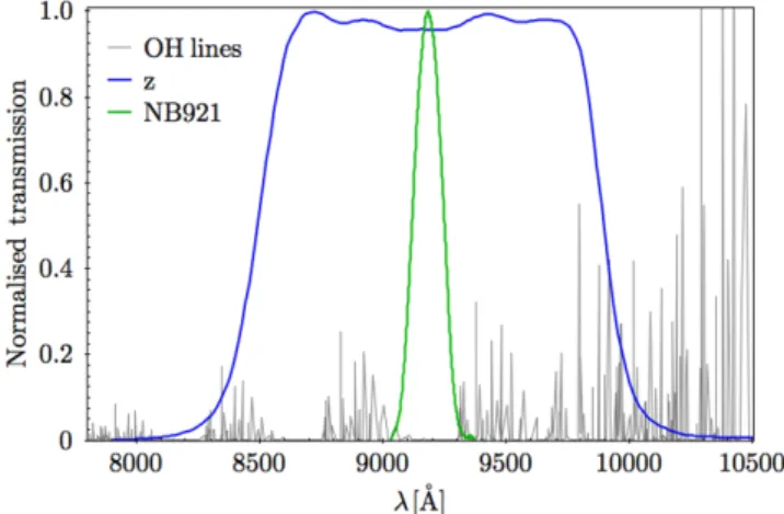
Optical imaging data were obtained with Subaru’s Suprime-Cam (Miyazaki et al. 2002) using theNB921 NB filter (Fig.1). The Suprime-Cam is composed by 10 CCDs with a combined field of view of 34 arcmin×27 arcmin and with chip gaps of∼15 arcsec. TheNB921 filter has a central wavelength of 9196 Å and an FWHM of 132 Å and is located in a wavelength region free of OH line emission in the atmosphere (see Fig.1).
We obtained archival ultradeep observations in UKIDSS-UDS (02 18 00−05 00 00) and COSMOS-UltraVISTA (10 00 00+02 00 00) and SA22 (22 00 00 +00 00 00) and took new data in a wide area (∼4.5 deg2) in SA22 on 2014 May 28–29,
Figure 1. Filter transmission profile of theNB921(blue) andz(green). The transmission is normalized to the maximum transmission in each filter. In grey, OH emission lines from the night sky are shown (Rousselot et al.
2000). It can be seen that the NB is in sky-line free region allowing us to go very deep. This also facilitates the spectroscopic follow-up.
of ultradeep and shallower surveys allows us to sample a wide range of luminosities.
In UDS, there are five subfields with a total integration time ranging from 7.8 to 10.5 h (see Table1). This exposure time is obtained after stacking individual exposures of 1.2 ks, with a small dithering pattern. The seeing FWHM ranges from 0.8 to 0.9 arcsec. We mask regions around bright stars, where spherical artefacts boost the fluxes artificially. We also mask horizontal and vertical stripes caused by blooming of a saturated bright object (see Fig.3). This is the same raw data as used to study LAEs atz=6.6 by Ouchi et al. (2010).
In the four pointings in COSMOS, the total integration time ranges from 2.2 to 3 h, with individual exposure time of 1.2 ks, such that the total number of exposures per field is smaller (ranging from 7 to 9). In two pointings, the seeing is particularly good (0.3 arcsec), the other two have seeing FWHM of 0.6 arcsec. Similar to in UDS, we mask spherical halo regions around bright stars, and vertical and horizontal blooming stripes (depending on the position angle rotation of the Suprime-Cam pointing).
The deep SA22 data consist of 27 exposures of 1.2 ks at a single pointing with small dithering in perfect seeing conditions (FWHM 0.3 arcsec). We mask a small noisy region and blooming patterns.
The wide SA22 data consist of 19 pointings of three exposures of 120 s in very good seeing conditions (FWHM 0.5 arcsec). Because of the limited number of exposures, a significant area has a lower signal to noise due to the dithering pattern. Another minor issue is that the astrometric corrections and calibration of the zero-point (ZP) are less accurate in certain detectors due to the low signal to noise. We conservatively mask all these regions and also mask regions around bright stars and are left with a final coverage of 2.7 deg2.
The total area after masking is 4.66 deg2. An overview of the
observations is given in Table1.
2.2 Data reduction
The NB921 imaging data were reduced with SDFRED2 package
(Ouchi et al.2004). The sequential steps in the reduction are as follows.
(i)Overscan and bias subtraction: for each image, a median value for the overscan region was determined and subtracted in each line of pixels. The bias was subtracted by assuming that it has the same value as the overscan.
(ii) Flat fielding: flat frames are obtained by observing a uniform light source and are required to correct variations in pixel-to-pixel sensitivity across the camera. By dividing the images by these flat frames, the background becomes flat and luminous patterns caused by differences in the sensibility of the pixels are removed.
(iii)Point spread function homogenization: the point spread func-tion (PSF) measures the response of the detector to a point-like source. PSF sizes were obtained by measuring the FWHM of the point-like sources of each frame. The target PSF for homogenisa-tion was defined as the one with more occurrences and the frames with PSF smaller than the target were smoothed with a Gaussian.
(iv)Sky background subtraction: a mesh pattern was computed to represent the sky background, the pattern was interpolated and subtracted on each frame.
(v)Bad pixel masking: defects with the detector and problems with the observations may cause data in some pixels to become corrupted. A mask is applied to these pixels.
(vi) Astrometric calibrations: we correct each image for astro-metric distortions using SCAMP(Bertin 2006), which fits a
poly-nomial solution by matching detected sources with the 2MASS catalogue in theJband (Skrutskie et al.2006). It also takes into
Table 1. Observation log for theNB921 optical imaging in the COSMOS, SA22 and UKIDSS UDS fields. Depths are based on empty aperture measurements and take correlations in the background into account. The UDS data have been analysed by Ouchi et al. (2010). The area is the area after masking (see Section 2.1).
Field R.A. Dec. Int. time FWHM Area Depth Dates
(J2000) (J2000) (ks) (arcsec) (deg2) (3σ)
COSMOS-1 10 01 28 +02 25 51 10.8 0.3 0.24 25.8 2009 Dec 19
COSMOS-2 09 59 35 +02 27 01 8.78 0.3 0.24 25.9 2009 Dec 19, 20
COSMOS-3 10 01 24 +01 58 00 10.8 0.6 0.24 25.9 2009 Dec 21
COSMOS-4 09 59 29 +01 58 42 7.80 0.6 0.24 25.7 2009 Dec 21
SA22-DEEP 22 19 14 +00 11 24 32.1 0.3 0.17 26.4 2009 Sept 15–17
SA22-WIDE-[1–19]* 22 16 19 +00 10 00 0.36 0.5 2.72 24.3 2014 May 28–29
UKIDSS-UDS C 02 18 00 −05 00 00 30.0 0.8 0.14 26.4 2005 Oct 29, Nov 1, 2007 Oct 11,12 UKIDSS-UDS N 02 18 00 −04 35 00 37.8 0.9 0.18 26.4 2005 Oct 30, 31, Nov 1, 2006 Nov 18, 2007 Oct 11, 12 UKIDSS-UDS S 02 18 00 −05 25 00 37.1 0.8 0.19 26.4 2005 Aug 29, Oct 29, 2006 Nov 18, 2007 Oct 12 UKIDSS-UDS E 02 19 47 −05 00 00 29.3 0.8 0.16 26.4 2005 Oct 31, Nov 1, 2006 Nov 18, 2007 Oct 11, 12 UKIDSS-UDS W 02 16 13 −05 00 00 28.1 0.8 0.14 26.4 2006 Nov 18, 2007 Oct 11,12
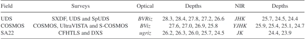
Table 2. 3σdepths of BB coverage of our survey fields obtained using empty aperture measurements. Note that there can be more wavelength data available, but we only use the BBs listed here for consistency between the fields. We obtain our own photometry by first registering all the images to theSubaru NB921 measurements and then extracting photometry within 2 arcsec apertures in dual mode. The SXDF data are presented in Furusawa et al. (2008), the COSMOS data in Ilbert et al. (2009) and UltraVISTA in McCracken et al. (2012).
Field Surveys Optical Depths NIR Depths
UDS SXDF, UDS and SpUDS BVRiz 28.3, 28.4, 27.8, 27.2, 26.6 JHK 25.7, 24.5, 24.4 COSMOS COSMOS, UltraVISTA and S-COSMOS BViz 27.6, 27.0, 26.9, 25.8 YJHK 25.9, 25.4, 25.1, 24.7
SA22 CFHTLS and DXS ugriz 26.2, 26.3, 26.0, 25.7, 24.5 JK 24.4, 23.9
account that images have different integration times and attributes a different weight to each image.
(vii)Stacking: once each individual frame has been reduced, we stack the different jittered frames for each pointing.
(viii)Cosmic ray rejection: cosmic rays are rejected automati-cally based on the standard deviation in the pixel values in a 1 arcsec aperture. The standard deviation is typically a hundred times higher for cosmic rays than for real sources. We use a very conservative cut since we do not want to risk rejecting real sources, meaning that our sample will still be somewhat contaminated by cosmic rays. Partly because of this, we inspect all our final candidates visually.
2.3 Photometric calibration and survey depths
Once we obtained the reduced data for each pointing, we set the ZP to a magnitude of 30 (AB). This is done by extracting sources with SEXTRACTOR(Bertin & Arnouts1996) with high detection thresholds
(>20σ) and match these sources with public catalogues in UDS (Cirasuolo et al.2007), COSMOS (Ilbert et al.2009) and our own catalogue in SA22 (based onKdetected sources in UKIDSS-DXS; Matthee et al.2014; Sobral et al.2015b), usingSTILTS(Taylor2006).
We only include sources with NB magnitudes brighter than 19, such that our detections are at sufficient high signal to noise, and fainter than 16, since brighter sources are saturated in our data. In each pointing, we use roughly 500 sources. We then set the ZP by correcting the cropped mean difference between the magnitudes in our images and the ones in the catalogue.
We estimate our survey depth by measuring the root mean square (rms) of the background in a million empty apertures with 2 arcsec diameters, placed at random places in the image, avoiding sources which are detected at>3σ. Empty aperture measurements take into account that the background noise is correlated and are thus more robust than if the background is measured on a pixel by pixel basis (cf. Milvang-Jensen et al.2013). Also, empty apertures can still include very faint sources below our detection threshold, so this is a conservative upper limit. The depths of the NB images are listed in Table1. The 3σdepths are 26.4 in UDS, 25.8 in COSMOS, 26.4 in the deep pointing in SA22 and 24.3 in the wide pointings in SA22.
2.4 Multiwavelength data and photometry
For UDS, deepz-band data (26.6, 3σ) are available from the Subaru Extreme Deep Field (SXDF) project (Furusawa et al.2008), as well as data in the optical bandsB,V,Randi, with 3σlimits: 28.3, 28.4, 27.8 and 27.2, respectively (see Table2). This multiwavelength data are essential to identify different line emitters. The images in the optical andNB921 are all aligned, because all are from a single survey, telescope and instrument. Furthermore, UKIDSS NIR J,H,Kdata (Lawrence et al.2007) are available for 60 per cent of the coverage, with 3σ depths 25.4, 24.7 and 24.9. For NIR
photometry, we useSWARP(Bertin2010) to align the NIR images to
theNB921 images and interpolate the NIR images, since the pixel scale is slightly larger (UKIRT WFCAM; Casali et al.2007) than the Suprime-Cam pixel scale.
The COSMOS field is one of the best studied extragalactic fields
with>30 bands coverage (Ilbert et al.2009), ranging from X-ray
to radio. We use deep opticalBVizdata fromSubaruimaging, with 3σ depths of 27.6, 27.0, 26.9 and 25.8 (Table2) which is avail-able through the COSMOS archive.1We align the optical images
to the NB images usingSWARP. NIR data inYJHKsare available
from UltraVISTA DR2 (McCracken et al. 2012) with 5σ depths 25.4, 25.1, 24.7 and 24.8. The pixel scale of VISTA’s VIRCAM is 0.15pixel−1, so we degrade the images to the pixel scale of the
NB images (0.2pixel−1) and align them.
The SA22 field is covered by CFHTLS and UKIDSS DXS sur-veys. SA22 is W4 in CFHTLS2and is imaged inugrizwith
Mega-Cam, which has a field of view of 1×1 deg2and a pixel scale of
0.187 arcsec pixel−1. The NIR UKIDSS DXS survey has imaged
it in Jand Kfilters with UKIRT/WFCAM. Note that the multi-wavelength data are not as deep as in the other two fields (typically 1–2 mag shallower), and there is also noSpitzer/IRAC data avail-able. This limits the search for LAEs in the deep pointing since the uncertainty in thezband is much higher than the uncertainty in NB921. For the brightest objects (including all reliable detections in the Wide coverage), this is less of a problem. As before, we align the optical and NIR images to our NB pointings usingSWARP, including degrading the pixel scale to that of the NB imaging.
For all fields, photometry is extracted using SEXTRACTORin dual-mode with theNB921 image as detection image and within a 2 arcsec circular aperture. In the case of a non-detection in any of the BBs, we assign 1σ limits. We then use theiband to correct ourzband such that the median NB excess is zero for all sources by fitting a linear relation between the (i−z) colour and the NB excess. Since the NB filter is almost in the centre of the BB filter, the correction is small,zcor=z−0.13(i−z)+0.286. For sources undetected in
theiband, we assign the median correction of+0.03.
3 S E L E C T I N G L A E S AT z=6.6
In theNB921 data, LAEs need to be selected as line emitters at z=6.55±0.055. This requires multiwavelength coverage of the fields, which is available through a combination of large (public) surveys. First of all, we require BB photometry over the same wavelength coverage as the NB, which is in this case thezband.
Line emitters are selected based on two criteria (e.g. Sobral et al.
2013): the first is that the NB excess must be high enough. Since the observed EW of emission lines increases with redshift and the
intrinsic EW of Lyαis high (∼100–200 Å), we expect LAEs to have a high NB excess. We follow previous searches (e.g. Ouchi et al.
2010) and use an excess criterion ofz−NB921>1, corresponding to a z = 6.6 rest-frame EW of 38 Å. This limit is also chosen to minimize contamination by lower redshift interlopers, although we will also lower this criterion and comment on the differences. To convert the NB excess to the observed EW, we first transform magnitudes (mi) to flux densities in each filter (fi) with the standard
AB convention:
fi= c
λ2
i,centre
10−0.4(mi+48.6).
(1)
In this equation,cis the speed of light andλi, centreis the central
wavelength in each filter, which are 9183.8 and 8781.7 Å for the NB and BB, respectively.
Using equation (1), we use the following equations to convert to EW and line flux, respectively:
EW= λNB
fNB−fBB
fBB−fNB λ λNBBB
. (2)
Here, fNB and fBB are the flux densities, λNB and λBB the
filter widths, 135.1 and 1124.6 Å, respectively. In this formula, the numerator is the difference in NB and BB flux and the denominator the continuum, which is corrected for the contribution from the NB flux. The formula breaks down at a certain NB excess depending on the specific filters, and thus we set the EW of those sources to >1500 Å.
The line flux is computed using
fline= λNB
fNB−fBB
1− λNB
λBB
. (3)
The second criterion for selecting emission line galaxies is that the excess should be significant, meaning that it is not dominated by errors in the NB and BB photometry. We will follow the methodol-ogy presented in Bunker et al. (1995) and the equation from Sobral et al. (2013) to compute the excess significance ():
= 1−10−0.4(BB−NB)
10−0.4(ZP−NB)
πr2 ap(σ
2 px,BB+σ
2 px,NB)
. (4)
In this case, BB is thez-band magnitude after correction using the iband (see the next subsections), NB the magnitude inNB921, ZP the zero-point of the images, which is set to a 30 AB magnitude. σpx is the rms of background pixel values in the data of the
re-spective filters andrapis the aperture radius in pixels. Our depths
are estimated using empty aperture-based rms values, which takes correlations in the background into account. For the selection of emitters, however, we use pixel-based rms values for consistency with previous surveys, but also check that our results are robust when using empty aperture-basedvalues.
After selecting a sample of line emitters, we use multiwavelength data to distinguish high-redshift candidate LAEs. In addition to the zband, we also need bands in bluer wavelengths in order to apply the Lyman-break technique to select high-redshift sources. In this case, this means that there should be no detection in theB,V,u, gandrfilters and a strong break in the (i−z) colours. Measure-ments in redder wavelengths, such as in the NIRJ,HandKfilters, can provide valuable insight in the nature of the candidates and possibly help excluding lower redshift interlopers. Finally,Spitzer -IRAC data can be used as further constraints on excluding dusty low-redshift interlopers (generally with bright IRAC detections and red colours), or as a further evidence for the source being atz=6.6,
since at that redshift the [3.6] and [4.5]μm bands are contami-nated in such a way that sources with strong nebular emission (EW
>1000 Å) are expected to have blue [3.6]−[4.5] colours (e.g. Stark
et al.2013; Smit et al.2014,2015).
In addition to using colours for our selection and characteri-zation of Lyαcandidates, we also compute photometric redshifts usingEAZYv1.1 (Brammer, van Dokkum & Coppi2008), which
includes the contribution of emission lines (although typically not strong enough for the observed extreme emission lines galaxies). We include optical and NIR photometry and we use it to identify possible lower redshift interlopers.
The details of our selection per field are presented in Section 3.1 for UDS, Section 3.2 for COSMOS and Section 3.3 for SA22.
3.1 Selecting LAEs in UDS
We use our photometry described in Section 2.4 and select line emitters using the following criteria:
(i)z−NB921>1
(ii) >3
(iii) Pass visual inspection
After the first two criteria, we have 1514 line-emitter candidates (see Table3for the numbers after each step). We check each line-emitter candidate visually in theNB921 image and exclude 122. Furthermore, 25 candidates are excluded since their excess is un-physically high, meaning that their (non-)detection in thezband is in disagreement with the flux solely contributed by the measured NB flux by more than 3σ. Most of the excluded candidates have their flux boosted by artefacts from bright stars, such as haloes or spikes (even after masking), others are excluded because they reflect read-out noise (since the images are so deep) and there are CCD grid-like patterns.
In total, we find 1367 line emitters, which selection is shown in Fig.2. This sample is dominated by Hβ/[OIII] atz=0.83, [OII]
emitters atz=1.46 and Hαatz= 0.40 (based on photometric redshifts), even though the high excess criterion is already used to minimize this number. These lower redshift emitters are described for example in Sobral et al. (2013), which also shows a photo-metric redshift distribution. To select Lyαcandidates, we exclude low-redshift sources and select high-redshift candidates using the Lyman-break technique:
B >28.7∧V >28.2∧(i−z >1.3∨i >27.2).
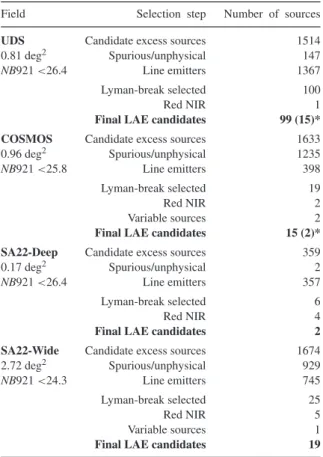
Table 3. Number of sources in each selection step, for each field. The final numbers of LAE candidates are printed in bold. When comparing the fields, it can be seen that there are relatively more line emitters selected as high-redshift source in UDS. This is because the UDS observations are deeper and the sample therefore exists of fainter observed sources, which generally are at higher redshifts. The number of interlopers identified based on NIR colours is rela-tively high in SA22, where the constraints on the Lyman break are weaker due to shallower optical photometry. We could only check for variability in the COSMOS field and a small part of the SA22 field.
Field Selection step Number of sources
UDS Candidate excess sources 1514
0.81 deg2 Spurious/unphysical 147
NB921<26.4 Line emitters 1367
Lyman-break selected 100
Red NIR 1
Final LAE candidates 99 (15)*
COSMOS Candidate excess sources 1633
0.96 deg2 Spurious/unphysical 1235
NB921<25.8 Line emitters 398
Lyman-break selected 19
Red NIR 2
Variable sources 2
Final LAE candidates 15 (2)*
SA22-Deep Candidate excess sources 359
0.17 deg2 Spurious/unphysical 2
NB921<26.4 Line emitters 357
Lyman-break selected 6
Red NIR 4
Final LAE candidates 2
SA22-Wide Candidate excess sources 1674
2.72 deg2 Spurious/unphysical 929
NB921<24.3 Line emitters 745
Lyman-break selected 25
Red NIR 5
Variable sources 1
Final LAE candidates 19
Notes.∗The number between parentheses shows the number of spec-troscopically confirmed LAEs.
additional step is not applied by Ouchi et al. (2010), but it makes little difference for these luminosities. It is however important for shallower NB surveys, as will be shown in the following sections. The public SpUDS-IRAC catalogue (Kim et al.2011) is based on a conservative magnitude limit and therefore does not contain faint enough objects, such that there is no match with any of the LAE candidates within a 2 arcsec radius, not evenHimiko. It is however detected in deeper IRAC data (Ouchi et al.2013).
We find a total of 99 Lymanαcandidates in UDS and show the positions in the UDS panel in Fig.3. The size of the symbols of the Lyαcandidates scales with the logarithm of the line flux.
3.1.1 Lowering the EW criterion
We retrieve 37 additional LAEs by lowering our excess (EW) cri-terion toz−NB921>0.5, but keeping the other conditions fixed. The risk of lowering the EW criterion is that the number of lower redshift interlopers increases. We use the NIR information and pho-tometric redshift to exclude lower redshift interlopers, because these will generally be very dusty (in order to mimic the Lyman break),
and thus bright and red in the NIR. In Section 3.1, we found only one interloper if we use an excess criterion ofz−NB921=1. If we lower the criterion toz−NB921>0.5, we remarkably find only four interlopers, where we expected to find more. However, most of the additional 37 LAEs are very faint in thezband, with magnitudes of∼25.5. This means that they need to have a very red colour (z−J>1 orz−K>2) to be detected in the NIR, since our detection limits are∼24–25 (see Table2). Therefore, it is likely that a fraction of interlopers which do not have those extreme colours might be missed. Because of their low excess, the additional LAEs have faint luminosities and thus affect mostly the faint end slope in the LF. However, since we do not include these luminosities in the LF due to their low completeness, the specific EW criterion used has little to no effect in our results.
3.1.2 Comparison to Ouchi et al. (2010)
The UKIDSS-UDSNB921 data have been analysed by Ouchi et al. (2010), who found 207 LAE candidates in UDS. The difference of 108 in number of candidates arises since we are even more con-servative in our masked regions, limiting magnitude and visually checking each candidate. However, when applying an analysis sim-ilar to Ouchi et al.’s, we find a very simsim-ilar LF (see Sections 5.1 and 5.2). From the 16 spectroscopically confirmed LAEs by Ouchi et al. (2010), we have 15 LAEs in our first selection. The remaining source has a slightly lower excess in our analysis because we do not useMAG-AUTO. Even though Lyαis sometimes observed to be
more extended than continuum emission (e.g. Steidel et al.2011; Momose et al.2014), we choose to use aperture photometry for all our measurements. This is motivated by our line-flux completeness estimate in Section 5.1 and a comparison with detection complete-ness in Section 5.1.1. However, by lowering our excess criterion to 0.9, we also select this source. Since we recover the LF and the spectroscopically confirmed LAEs, we find that our sample of LAEs is in agreement with the sample from Ouchi et al. (2010) and that we fully recover their results.
3.2 Selecting LAEs in COSMOS
With the photometry presented in Section 2.4, we select line emitters in the COSMOS field using
(i)z−NB921>1
(ii) >3
(iii) Pass visual inspection
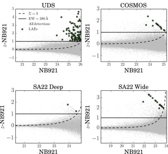
Figure 2. NB excess versus NB magnitude. This figure shows the selection of line emitters in our different fields. The grey points show all detected objects (after removing cosmic rays, visually identified spurious sources and sources for which the excess is unphysical) and the green points show the selected LAEs in each field. The selection consists of an EW cut (solid horizontal line) and a criterion to determine whether the excess is significant (dashed lines). The EW cut corresponds to a rest-frame EW of 38 Å atz=6.56, and the significance cut corresponds to 3. After visual removal of spurious sources and cosmic rays and optical and NIR BB criteria, we find 99 LAEs in UDS, 15 in COSMOS, 2 in SA22-Deep and 19 in SA22-Wide. While the NB imaging in UDS and SA22-Deep have similar depth, the number in UDS is higher due to a roughly five times larger area and (most importantly) deeperz-band imaging. There are less candidates in COSMOS due to shallower NB imaging. The imaging in SA22-Wide is even shallower, but this is compensated by a much larger area.
use COSMOS for brighter sources. They agree in number densities (Fig.4) indicating that this approach is correct.
In total, we have 398 line emitters. The photo-zdistribution is peaked at [OIII]/Hβ atz=0.83, with a smaller peak at Hαat
z=0.40 and one around [OII] atz=1.46. 10 have spectroscopic
redshifts, of which 9 are [OIII]/Hβand 1 [OII], see Sobral et al. (2013). In order to select LAEs, we apply the following criteria to select high-redshift line emitters (see also Section 3.1):
B >27.9∧V >27.3∧(i−z >1.3∨i >27.0)
The optical limits are 2σlimits (also applied to UDS) computed by our empty aperture measurements, but consistent with Muzzin et al. (2013). We use the deep NIR data to identify dusty lower redshift interlopers with red NIR colours and identify two likely [OIII] or [OII] emitters, which haveJ−K= 1.53 andJ− K=1.8 and
observed EW of 420 and 350 Å, respectively.
In addition to this, we are able to check our sources for variability. We have publicly available data from Sobral et al. (2013) which have been taken one year later than the COSMOSNB921 data and reaches a 3σ depth of∼25, which is similar to the magnitudes of our faintest Lyαcandidates. By comparing the magnitudes, we exclude the two brightest candidates (NB921∼21.5), because they
are completely undetected in the data from Sobral et al. (2013). This means that their brightness changes by∼5 mag and that they are thus likely supernovae (SNe). This means that similar surveys are expected to have roughly two SNe per 0.9 deg2as contaminants
to their sample of LAEs, except if the data have been split over multiple epochs. This may be very important to interpret results at higher redshift (e.g. Faisst et al.2014; Matthee et al.2014) and shows how important it is to have data spread over time.
We match our remaining LAE candidates to sources in the S-COSMOS-IRAC catalogue and find one match. This match is our brightest candidate, nicknamed ‘COSMOS REDSHIFT 7;CR7’. After these steps, we find 15 Lymanαcandidates in COSMOS, of which two remarkably bright sources – brighter thanHimiko– and show their positions in Fig.3. The size of the symbols of the Lyα
candidates scales with the logarithmic of the line flux.
Figure 3. Position on the sky of the three survey fields. The three panels show the relative areas of the three fields. Grey dots show all detections with NB921<22 (chosen in order to control the file size of the images), highlighting the masked regions due to bright stars as empty circles and masked noisy areas which are due to our pointing strategy (such as the grid pattern in SA22). In SA22, the detections in the Deep region have a slightly darker colour. The green symbols show the positions of our LAEs. The size of these symbols scales with the line flux (luminosity), following size∼(log10(LLyα))3/5, and has
the same limits and range for all the three fields. From this, it can be seen that UDS is significantly deeper since it has many more LAEs with small symbols. We furthermore note that two LAE candidates in SA22 are not visible in the image because they overlap with other symbols due to a small separation on the sky (∼4 arcsec).
3.2.1 Spectroscopic follow-up: bright sources in COSMOS
In UDS, there are 16 spectroscopic confirmed LAEs by Ouchi et al. (2010) using Keck/DEIMOS. For COSMOS, we have ob-tained spectroscopic follow-up for our brightest two candidates us-ing Keck/DEIMOS and DDT programme 294.A-5018 on VLT/X-SHOOTER and VLT/FORS2 presented in Sobral et al. (2015a). Both of these are confirmed LAEs, at redshifts z = 6.604 and 6.541, respectively. We nicknamed these galaxiesCR7(see above) andMASOSA.3CR7is detected at only half of the NB filter
trans-3The nicknameMASOSAconsists of the initials of the first three authors of
this paper.
mission, leading to a 2 arcsec luminosity of 5.8×1043 erg s−1,
which is a factor 2 higher than our estimate from the photome-try. Based onMAG-AUTO, the luminosity is 9.6×1043erg s−1, and
thus a factor 2.5 brighter thanHimiko. This is a lower limit since the COSMOSNB921 observations are shallower than in UDS and might therefore miss some lower surface brightness regions and it assumes thez-band continuum being flat. It is so extreme that it is even detected individually in thezYJHKbands and detected at 5σ in the NIR stack, withYJHK=24.9. It is also detected in IRAC, with a blue [3.6]−[4.5] colour, consistent with the [3.6]μm flux being boosted by strong Hβ/[OIII] line emission (e.g. Smit et al.
Figure 4. Number counts in our three fields, compared to the bins from Ouchi et al. (2010). The bins are only corrected for completeness. Our bins in UDS vary with this from Ouchi et al. (2010) because we use luminosities based on 2 arcsec apertures and apply a different completeness correction. The SA22-Wide bins are corrected for contamination from variable sources and SNe, empirically calibrated in COSMOS. Note good agreement between measurements from all fields, although some variance is found which is likely due to cosmic variance.
catalogues from Bowler et al. (2012,2014). However, the LyαEW is much larger than the values used for the SED fitting (see Sobral et al. 2015a), meaning that the result from their SED fit requires revision and explaining the highχ2.
MASOSA(with a Lyαluminosity of at least 3×1043erg s−1,
both in a 2 arcsec aperture andMAG-AUTO) is not detected in any
of the NIR bands, and also not in the stacked image (meaning YJHK>26.7).MASOSAis undetected in thezband, meaning that the luminosity is a lower limit. It is only brighter thanHimikowhen measured in 2 arcsec apertures, but this could also be due to our fainter NB imaging in COSMOS than in UDS. It is not extended (diameter∼0.9 arcsec), whileCR7andHimikoshow an extent of ∼3 arcsec in diameter. This means that the sources are of a different nature and therefore interesting targets for follow-up study with e.g.HST.
None of our LAE candidates are in the zCOSMOS (Lilly et al.
2009) or UDSz (Bradshaw et al.2013; McLure et al.2013) cata-logues, which we also did not expect, since they would likely be interlopers in that case. As expected, none of our LAE candidates except forCR7are in the UV-selectedz∼7 galaxy catalogue from Bowler et al. (2014), since they are not detected in BB photometry. None of the other sources in the Bowler et al. (2014) catalogue are selected as line emitters.
3.3 Selecting LAEs in SA22 Wide and Deep
Using our photometry described in Section 2.4, we select line emit-ters using the following criteria:
(i)z−NB921>1
(ii) >3
(iii) Pass visual inspection
After these steps, we find 1674 line emitters in SA22-Wide, from which we exclude 359 for having an unphysically high excess, and
347 emitters in SA22-Deep (see the corresponding panels in Fig.2, and Table3) and apply the following criteria to select high-redshift line emitters:
u >26.4∧g >26.5∧r >26.2∧(i−z >1.3∨i >25.9).
The optical limits are 2σ limits and the (i−z) criterion is similar to that in the other fields. We visually check each LAE candidate in theNB921 images and exclude a further 560 in SA22-Wide and 2 in SA22-Deep. Most of these objects are cosmic rays which were not detected automatically and sources which have their flux boosted by haloes or spikes caused by bright stars are thus not real excess sources. In SA22-Wide, our-value from pixel-based measurements corresponds to a 3if we measured the background with empty apertures, and to 1.5in SA22-Deep. These differences are caused by a different limiting NB magnitude.
There is one LAE candidate in SA22-Wide which is in the small overlapping region with SA22-Deep. This source happens to be variable, as it is undetected in the SA22-Deep data. We could not check the major part of the SA22-Wide field for variability and therefore use a statistical correction to the LF using our empirical results from the COSMOS region, where we found two variable sources (likely SNe) per 0.9 deg2. The area is 2.72 deg2, so we
weight our number densities down by six sources.
Since the optical photometry in SA22 is shallower than in the other fields (see Table2), there is a higher chance of our candidates being lower redshift interlopers, since the Lyman-break constraints are not as stringent. Using the NIRJandKdata, we identify objects with significantly red NIR colours (J−K>0.5). In SA22-Deep, we exclude four out of our six LAE candidates based on optical colours only, and are thus left with two LAEs. These four lower redshift interlopers can be called extreme emission line galaxies, since their observed EW is∼400 Å. In SA22-Wide, we exclude five interlopers out of the 24 LAE candidates from the NIR photometry. Because the SA22-Wide candidates are brighter, possible interlopers are easier to exclude based on their optical colours. Therefore, this number is relatively lower than in SA22-Deep. In total, we find 2 LAEs in SA22-Deep, and 19 LAE candidates in SA22-Wide. Their spatial position is shown in Fig.3, where the size of the symbols scales with the logarithm of the line flux.
The LAE candidates in SA22-Wide are particularly bright, with luminosities 3–16×1043erg s−1, if they are atz=6.6. We note
that four candidates are in pairs which are separated only by∼3– 5 arcsec in the sky (such that only one point is seen in the Fig.3). Once these candidates are spectroscopically confirmed, this sample will allow us to study the variety of bright LAEs.
4 N U M B E R C O U N T S , C O M P L E T E N E S S A N D C O R R E C T I O N S F O R F I LT E R P R O F I L E B I A S
by the fraction of the sky that is our survey area. We find a comoving volume of 9.02×10⁵Mpc3deg−2, corresponding to 7.4×10⁵Mpc3
in UDS, 8.7×10⁵Mpc3in COSMOS, 1.5×10⁵Mpc3in
SA22-Deep and 2.5×10⁶Mpc3in SA22-Wide. In total, our volume is
42.6×10⁵Mpc3.
4.1 Line-flux completeness
Our selection of line emitters relies on the measured NB excess and the excess significance. This means that photometric errors can lead to missing real LAEs atz = 6.6, especially at the faintest luminosities. The result is that our sample is incomplete. How in-complete our survey is at a given luminosity (line flux) depends on the survey depth, source extraction and selection method. We can measure the incompleteness with a simulation based on a sample of observed sources which are consistent with being at high redshift (z >3, using Lyman-break criteria), but are not detected as line emitters. This sample is detected and analysed in exactly the same way as our sample of Lyαcandidates and has similar NB magni-tude distribution. To these sources (>1000 in total in the three deep fields, and>10 000 in SA22-Wide), we artificially add line flux by changing theirNB921 andz-band magnitude correspondingly, and test whether it is then selected as a line emitter based on the updated excess and excess significance. The completeness is then obtained for each line flux by measuring the fraction of sources which is selected as line emitter after adding the flux (e.g. Sobral et al.2012). We measure the completeness in the three deep fields for each pointing, but averaged over the SA22-Wide pointings. Be-cause of the limited depth of SA22-Wide, there are less number of sources per pointing and the statistics is thus weaker. We find that the completeness in different pointings in UDS and COSMOS are very similar. We show the line flux for which each of our fields is complete up to 80 per cent in Table4. These fluxes correspond to lu-minosities from 6.37×1042erg s−1(UDS) up to 4.9×1043erg s−1
(SA22-Wide). Note that even though the NB photometry has similar depths in SA22-Deep and UDS, the line-flux completeness is very different due to a different BB limit. This means that a measure of completeness based on detection only will give inconsistent results. For each luminosity bin, we correct the number of sources by dividing by the completeness. We also divide the Poissonian errors by this completeness value. Only bins with a completeness higher than 40 per cent are included in the LF. The completeness correction is strongest for the faintest luminosities, and thus increases the number density mostly at low luminosities.
Table 4. The line flux for which our completeness is 80 per cent, shown in our different fields. This depends on both theNB921 andz-band depths. Note that, because of this, even though the NB photometry has similar depths in SA22-Deep and UDS, the line-flux completeness is very different due to a different BB limit. This high-lights the need for line-flux completeness over detection completeness.
Field 80 per cent completeness flux UDS 1.3×10⁻¹⁷erg s−1cm−2
COSMOS 4.4×10⁻¹⁷erg s−1cm−2
SA22-Deep 7.4×10⁻¹⁷erg s−1cm−2
SA22-Wide 10.0×10⁻¹⁷erg s−1cm−2
4.1.1 Detection completeness in SA22
In order to access the quality of our data in our wide SA22 survey, we use our three spectroscopically confirmed bright LAEs to estimate the detection completeness. By placing them at random positions in our images and see whether we recover them, we know whether our data are sufficient to observe these luminous sources and we can furthermore check our line-flux completeness procedure (see above) and see how the two compare.
We produce small cutouts (5 arcsec ×5 arcsec) around CR7, HimikoandMASOSAand add them to 100 random positions per pointing in SA22, excluding masked regions. After this, we run SEXTRACTORwith identical settings as used on the original images
and compute the fraction of our input sources which is detected. We repeat this a 1000 times per image and use the average re-covered fraction as detection completeness. On average, we find a detection completeness of 44 per cent, with a standard deviation of 20 per cent in different pointings. The detection completeness is highest forMASOSA, 64 per cent, around the average for CR7, 43 per cent, and lowest forHimiko, 27 per cent. This is because the first source is not extended, while the other two are extended and therefore have lower surface brightnesses. Note that we do not ex-clude pixel positions with actual sources or regions with a slightly lower signal to noise, which both decreases the completeness. The average detection completeness is remarkably similar to our esti-mated line-flux completeness (which is 46 per cent for the average line flux of the three sources). The large variation in detection com-pleteness between the different sources, which have almost the same 2 arcsec magnitude, highlights the need for a completeness based on line flux, instead of detection.
4.2 Number densities
We show our number densities in Fig.4 and compare with the number densities from Ouchi et al. (2010, purple circles), which is based majorly on UDS. Our UDS points agree with those of Ouchi et al. (2010), while the SA22-Deep and COSMOS bins (which are spectroscopically confirmed) converge at brighter luminosities and are also consistent with Ouchi et al. (2010). Our SA22-Wide num-ber densities are more uncertain, since there is no spectroscopic confirmation yet and the photometric constraints are weaker than in the other fields. However, even if there are still some contaminants, these further highlight a departure from a Schechter function (al-ready indicated by our spectroscopically confirmed sample) at high luminosities and indicate that the observed LyαLF atz=6.6 can be fitted by a power law (e.g. the pentagons in Fig.4). The power-law fit is
log10(
Mpc−3)=68.38−1.68 log10
LLyα
erg s−1
.
Since we have only two sources in SA22-Deep and since this agrees very well UDS and COSMOS, we will include them when we refer to the UDS+COSMOS sample in the remainder of the text. We will also refer to the SA22-Wide results as SA22.
Table 5. Correction factors for the number densities at z=6.6. These corrections are made for the bias arising from the observations through the filter profile not being a top-hat. Because of the filter profile, luminous LAEs can be observed as faint LAEs, meaning that their real number densities are higher than observed. This is particularly important for when comparing NB LAE searches with IFU based LAE searches.
Luminosity bin Number density correction factor
42.5 0.99
42.7 1.07
42.9 1.18
43.1 1.32
43.3 1.51
43.5 1.77
43.7 2.08
43.9 2.79
therefore overestimate the bright end. We are aware of this bias, but do not apply a correction in order for consistency with previous surveys and since its effect are similar between different redshifts.
4.3 Filter profile bias correction
Since our filter is not a perfect top-hat, the exact redshift of the Lyα emission line influences the observed luminosity. This means that intrinsic luminous LAEs which are detected at the edges of the fil-ter (where the transmission is lower) are observed as fainfil-ter LAEs. It also means that the probed volume depends on the luminosity, since luminous sources can be detected over a larger redshift range, but will be observed as fainter sources. For example, our brightest spectroscopically confirmed source in COSMOS,CR7, is actually detected at only 50 per cent of the transmission and is thus even brighter than our photometric estimate. Corrections for this effect are derived with a simulation, similar to Sobral et al. (2013) for Hαline emitters. We use the Schechter fit of our UDS+COSMOS data to generate a million LAEs and assume that they have a ran-dom redshift between the edges of the filter. We then convolve the luminosities with the filter profile into an observed population. Corrections are then obtained by comparing the number of sources in each luminosity bin before and after applying the filter profile. The result of our correction is that the number density of luminous sources is increased, while it decreases at low luminosities. We note explicitly that this correction is required to remove the bias from observation strategy, since e.g. an Integral Field Unit (IFU) survey without a filter would not suffer from this bias, and that it is not related to any intrinsic effect of the sources. We show the correction factors forz=6.6 in Table5.
4.3.1 Comparison to Ouchi et al. (2010) and effect of the filter profile correction
There are two reasons for the small differences between our UDS and Ouchi’s number densities (Fig.4): the first is that our complete-ness correction is based on line flux and the selection of emitters, while their completeness correction is based on detection complete-ness and NB magnitudes. The other difference is that Ouchi et al. (2010) usesMAG-AUTOto estimate NB magnitudes (which are used
to compute luminosities), while we use the magnitude in 2 arcsec apertures. As Lyαis often extended,MAG-AUTOmight have been a
better choice. We however chose to consistently use the 2 arcsec
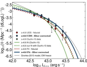
Figure 5. LF atz=6.6: comparison of number densities and fits with and without filter profile correction. We compare our number densities in UDS with those of Ouchi et al. (2010), which are largely based on the UDS field as well. We show that our red hexagons (before correcting for the filter profile) agree well with the green squares from Ouchi et al. (2010), whose fit to the data is shown as a solid green line. The dashed green line shows our fit to their total data (fixingα= −1.5 in equation 5), which differs significantly from their published fit. The fit to our data (αfixed to−1.5; dashed red line) again agrees well, indicating that our results are similar. The effect of the filter profile correction is shown by comparing the blue hexagons with the red hexagons. The effect is that the number density of bright line emitters is higher, while the number density of faint line emitter is slightly lower. The blue line shows the fit to the bins after correcting for the filter profile, which again highlights the effect of the correction. The grey line shows a model prediction by Gronke et al. (2015) which is based on the LBG LF and a Lyα
EW distribution, frozen atz=6.0. It is remarkable that there it agrees well with the blue curve, despite not being a fit.
aperture since we also used this for our (important) line-flux com-pleteness correction. UsingMAG-AUTOwould mean the introduction
of an additional uncertainty. We compare the luminosities derived with both 2 arcsec apertures and MAG-AUTO for the spectroscopic
confirmed sample in UDS and find that corrections of+0.11 dex can be used to statistically correct the luminosities. This is used in Fig.4and in all other following LFs. Our results do not strongly depend on this correction.
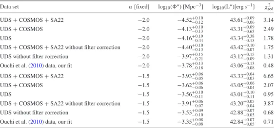
Table 6. Values to our Schechter fits to the LFs. Because of our limited depth, we fix the faint end slope to either−2 or−1.5 and only keep∗andL∗as free parameters.
Data set α[fixed] log10(∗) [Mpc−3] log10(L∗)[erg s−1] χred2
UDS+COSMOS+SA22 −2.0 −4.52−+00..1012 43.61+
0.09
−0.06 3.14
UDS+COSMOS −2.0 −4.13−+00..1013 43.31+−00..0965 2.49
UDS −2.0 −4.16−+00..1944 43.34+−00..3813 1.78
UDS+COSMOS+SA22 without filter correction −2.0 −4.40−+00..1013 43.42−+00..1007 1.75 UDS without filter correction −2.0 −3.97−+00..1521 43.12+−00..1509 1.31 Ouchi et al. (2010) data, our fit −2.0 −3.78+−00..1318 43.06+0
.13
−0.08 0.48
UDS+COSMOS+SA22 −1.5 −3.93−+00..0605 43.33−+00..0403 6.65 UDS+COSMOS −1.5 −3.62−+00..0606 43.05+−00..0604 2.07
UDS −1.5 −3.56−+00..1011 43.01+−00..1011 0.95
UDS+COSMOS+SA22 without filter correction −1.5 −3.91−+00..0607 43.20+ 0.05
−0.04 3.87
UDS without filter correction −1.5 −3.53+−00..0910 42.88+ 0.07
−0.05 0.68
Ouchi et al. (2010) data, our fit −1.5 −3.35−+00..0808 42.84+−00..0705 0.71
5 LYα L F AT z =6 . 6
In this section, we present thez=6.6 LyαLF from our combined analysis in UDS, COSMOS and SA22. As a functional form, we use the well-known Schechter function:
φ(L)dL=φ∗(L/L∗)αexp(−L/L∗)d(L/L∗). (5)
We convert our observed line fluxes to luminosities by assuming a luminosity distance corresponding to a redshift of 6.56, which is the redshift of the centre of the filter. We combine the luminosities in bins with widths of 0.2 dex and count the number of sources within each bin and correct this number for incompleteness. The errors on the bins are taken to be Poissonian. The number of sources is divided by the probed volume, such that we obtain a number density. We then apply our corrections for the filter profile bias. Only data where the completeness is at least 40 per cent are included. The resulting LF is shown in Fig.6, where we also compare with other published z=6.6 LAE data. The evolution betweenz=5.7 and 6.6 is shown in Fig.7, while the left-hand panel of Fig.8shows the evolution towardsz=7.3. We are cautious about interpreting the results from SA22 because of the less stringent photometric criteria, even though they fully agree with results from the other fields. The results from UDS and COSMOS, however, are confirmed by spectroscopy.
It is interesting to compare these results with the model from Gronke et al. (2015), which is shown as the black line in Fig.5. This model uses the UV LF and a probability distribution function (PDF) of LyαEWs to predict the LyαLF. The EW distribution generally evolves with redshift, but in this case, it is frozen to the EW PDF atz=6.0, because of possible effects from reionization. It is remarkable that the prediction from Gronke et al. (2015) seems to be consistent with our blue points. Differences arise because of their steeper faint end slope (∼−2.2), which is largely unconstrained by the depth of our current data of LAEs. The agreement highlights the need for the correction of the filter profile bias when comparing NB-derived LFs with LFs NB-derived from spectroscopy (either follow-up or blind IFU).
As noted in Section 5.2.1, our results in UDS differ by those from Ouchi et al. (2010) at brighter luminosities due to a different treatment of the brightest bin in the fit (solid green line) and by correcting for the filter profile (which effect is shown in Fig.5). This explains also the differences (although largely within the errors) with Kashikawa et al. (2006), although cosmic variance plays a role
Figure 6. The LymanαLF atz=6.6 compared to literature data. Our most robust LF is shown as a solid blue line. This is a Schechter fit to our combined UDS and COSMOS data (blue circles, see also Table6), for which the brightest LAEs have all been confirmed spectroscopically. Our additional SA22 data are shown in open circles and are consistent with the upper limits from our robust sample. We also place upper limits (blue and open arrow) at the luminosity bin just brighter than the most luminous observed sources, meaning that there is less than one of these in the probed volume. The dashed blue line is our power-law fit (see Table7) to the data from all three fields. The fit from Ouchi et al. (2010) atz=6.6 differs for two main reasons (see also Fig.5), namely practically not including the brightest bin to their fit (due to very large errors, as the fit contains only a single source) and not correcting for different biases caused by the filter profile. This is also the major reason why our results are slightly different with the results from Kashikawa et al. (2006, ochre diamonds) and Hu et al. (2010, red squares). Other reasons are cosmic variance, since they only probed small areas (Kashikawa et al.), and small (spectroscopic) completeness (Hu et al.).
Figure 7. Evolution of the LyαLF fromz=6.6 to 5.7. We compare our z=6.6 LF (blue solid line) to published data and fits to the data atz=5.7. We apply a filter profile correction to the data from Ouchi et al. (2008) at z=5.7 (green: uncorrected, ochre: corrected) and fit a Schechter function to the corrected data (orange solid line). We also show the spectroscopically confirmed results from Westra et al. (2006) atz=5.7. Comparing the orange solid line to the blue solid line shows that the LF evolves only at the faint end and not (as has been claimed by Ouchi et al. (2010)) at all luminosities. In fact, we find no evolution forL>1043.5erg s−1. We show in Section 6.2
that this may be a consequence of reionization. We do not show our fit which includes the SA22 data points, since there is no comparison available atz=5.7. This motivates the need for larger volumes atz=5.7 as well, in order to see if there is evolution at the bright end.
only slightly with the second brightest bin. Our SA22 results are not yet confirmed spectroscopically and are thus upper limits when viewed most conservatively. There is however excellent agreement with the spectroscopically confirmed COSMOS sources and with the upper limits from the UDS+COSMOS sample (blue arrow in Fig.6). If all (or even only a fraction) of these very bright LAEs in SA22 are confirmed, this indicates that the observed LyαLF at z=6.6 can be fitted by a power law (e.g. the pentagons in Fig.4), similar to the UV LF atz=6–7 (e.g. Bowler et al.2014).
Now we have used a combination of wide and ultradeep fields, established a new LF atz=6.6 (see Table6) and will compare this with results in the literature at lower redshift. To be conservative, we will use our fit to the UDS+COSMOS sample for comparison, although our results are only strengthened by the results from SA22.
5.1 The z=5.7−6.6 evolution of the LF
Previous studies (e.g. van Breukelen, Jarvis & Venemans 2005; Ajiki et al.2006; Shimasaku et al.2006; Gronwall et al.2007; Ouchi et al.2008) have found that the observed Lyα LF is remarkably constant betweenz=3 and 6. While the LBG LF declines over this redshift range, the implication is that the strength of the Lyαline increases with redshift, which is also confirmed spectroscopically (e.g. Stark et al.2010). Atz >6, there is evidence both from a declining success rate of spectroscopic observations of LBGs (e.g. Schenker et al.2012), and also for a drop in the LyαLF (Ouchi et al.
2010; Konno et al.2014). In our independent analysis, we confirm evolution of the LyαLF fromz=5.7 to 6.6, although only robustly at fainter luminosities,L<1043erg s−1, see Fig.7. As a comparison
atz=5.7, we use data points from Ouchi et al. (2008, green squares
Figure 8. Left: evolution of the LF evolution fromz=7.3 to 5.7. We compare ourz=6.6 LF (blue solid line) to published data atz >7 Konno et al. (2014) (red squares) Shibuya et al. (2012); Ota et al. (2010); Iye et al. (2006) (purple triangles, pentagons and diamond, respectively). We also show our LF fit to the correctedz=5.7 data (orange solid line) and the green squares show the number densities atz=5.7 from Ouchi et al. (2008). Note that the errors on the z >7 data are still significant and that the surveys are limited to small areas, meaning that the LF is still unconstrained at luminosities>1043.3erg s−1. A few
additional, shallower pointings with the Subaru S-Cam and theNB101 (z=7.3) filter would place useful constraints on the evolution of the LyαLF at these epochs. Right: toy model evolution of the LF in a neutral IGM. The black line shows the input LF, which is thez=5.7 LF from Ouchi et al. (2008). We fix the parameters controlling the age and number of escaping ionizing photons from LAEs (to age=100 Myr,fesc, ion=5 per cent andfesc, Lyα=30 per cent) and investigate how a changing neutral fraction (XH I) influences the observed LF. As can be seen, the evolution starts at the faintest luminosities only and gradually
towards higher luminosities. The highest luminosities (>1043.5erg s−1) are still observable. Faint LAEs are observable if they are in the ionized sphere of a