chabra_unc_0153D_19221.pdf

IMPROVING 3D RECONSTRUCTION USING DEEP LEARNING PRIORS

Rohan Chabra

A dissertation submitted to the faculty at the University of North Carolina at Chapel Hill in

partial fulfillment of the requirements for the degree of Doctor of Philosophy in the Department

of Computer Science.

Chapel Hill

2020

ABSTRACT

Rohan Chabra: IMPROVING 3D RECONSTRUCTION USING DEEP LEARNING PRIORS

(Under the direction of Henry Fuchs)

Modeling the 3D geometry of shapes and the environment around us has many practical

ap-plications in mapping, navigation, virtual/ augmented reality, and autonomous robots. In general,

the acquisition of 3D models relies on using passive images or using active depth sensors such

as structured light systems that use external infrared projectors. Although active methods

pro-vide very robust and reliable depth information, they have limited use cases and heavy power

requirements, which makes the passive techniques more suitable for day-to-day user applications.

Image-based depth acquisition systems usually face challenges representing thin, textureless, or

specular surfaces and regions in shadows or low-light environments. While scene depth

informa-tion can be extracted from the set of passive images, fusion of depth informainforma-tion from several

views into a consistent 3D representation remains a challenging task. The most common

chal-lenges in 3D environment capture include the use of efficient scene representation that preserves

the details, thin structures, and ensures overall completeness of the reconstruction.

ACKNOWLEDGEMENTS

There are key individuals that have provided me with the support and tools that a graduate

student could want. Here, I wish to acknowledge those friends, advisors, and relatives that have

guided and inspired me throughout this doctoral endeavour.

First and foremost, I would like to thank my supervisor, Prof. Henry Fuchs for giving me

an opportunity to be part of a unique research experience under his guidance. His experience,

expertise, and thoroughness is largely responsible for the quality of research in my dissertation. I

would like to thank my loving fianc´ee, Nirupama Sharma for being very supportive and patient

with me during my every struggle as a doctorate student. I am extremely grateful to my dearest

friend Aniket Bera for helping me throughout my graduate student life. He has been the source

of motivation for my pursuit to doctorate and has helped and guided me in achieving several

milestones during my doctoral journey.

I am extremely grateful to Dr. Richard Newcombe for giving me an excellent opportunity

to work with him and his team at Facebook Reality Labs during the course of several

intern-ships and research collaborations. This fortunate collaboration with Richard gave me a chance to

use the state-of-the-art research tools and an opportunity to work with an expert research team.

Richard, also guided me in the development of several innovative ideas and technical concepts

that became an integral part of this dissertation. This dissertation would not have been possible

without his immense support and guidance.

TABLE OF CONTENTS

LIST OF TABLES . . . .

xi

LIST OF FIGURES . . . xiii

LIST OF ABBREVIATIONS . . . xix

CHAPTER 1:

INTRODUCTION . . . .

1

1.1

Motivation and Problem Statement . . . .

1

1.2

Related Work . . . .

9

1.2.1

3D Reconstruction using Traditional Methods . . . .

9

1.2.1.1

Depth Estimation . . . .

9

1.2.1.2

3D Scene Representation Methods . . . 10

1.2.2

3D Reconstruction using Learning Based Methods . . . 10

1.2.2.1

Learning Depth Estimation . . . 11

1.2.2.2

3D Scene Representation Learning . . . 11

1.3

Thesis Contributions . . . 12

CHAPTER 2:

TECHNICAL INTRODUCTION . . . 14

2.1

Deep Learning for 3D Vision . . . 14

2.1.1

Deep Artificial Neural Networks . . . 15

2.1.1.1

Artificial Neuron . . . 15

2.1.1.2

Multi Layer Perceptrons (MLP) . . . 18

2.1.1.3

Convolutional Neural Networks . . . 18

2.1.1.4

Optimization Algorithms . . . 20

2.1.2

Datasets for 3D Learning . . . 23

2.2

Depth From Stereo Vision . . . 24

2.2.1

Stereo Camera Calibration . . . 25

2.2.2

Stereo Matching . . . 27

2.2.2.1

Feature Descriptors . . . 28

2.2.2.2

Correlation Metrics . . . 29

2.2.2.3

Disparity Estimation . . . 30

2.3

3D Surface Representations . . . 32

2.3.1

Signed Distance Function . . . 33

2.3.2

Surface Representation Methods . . . 34

2.3.2.1

Radial Basis Function (RBF) . . . 35

2.3.2.2

Multi-level Partition of Unity (MPU) . . . 35

2.3.2.3

Grid Sampling . . . 36

CHAPTER 3:

LEARNING BASED DEPTH ESTIMATION FROM STEREO . . . 38

3.1

Introduction . . . 38

3.2

Background . . . 39

3.3

StereoDRNet: Dilated Residual Stereo Net . . . 40

3.3.1

Key Contributions . . . 40

3.4

Algorithm . . . 41

3.4.1

Feature Extraction . . . 42

3.4.2

Cost Volume Filtering . . . 42

3.4.3

Disparity Regression . . . 44

3.4.4

Disparity Refinement . . . 45

3.4.5

Training . . . 48

3.5

Network Details . . . 48

3.6.1

SceneFlow Dataset . . . 52

3.6.2

KITTI Datasets . . . 53

3.6.3

ETH3D Dataset . . . 57

3.7

Conclusion . . . 58

CHAPTER 4:

3D RECONSTRUCTION FROM LEARNING BASED STEREO . . . 59

4.1

Introduction . . . 59

4.2

Indoor Scene Reconstruction . . . 60

4.2.1

Comparison with MVS . . . 65

4.2.2

3D Reconstruction Details . . . 67

4.3

Effect of Refinement. . . 67

4.4

Conclusion . . . 69

CHAPTER 5:

LEARNING LOCAL SDF PRIORS FOR DETAILED 3D

RECON-STRUCTION . . . 70

5.1

Introduction . . . 70

5.2

Related Work . . . 72

5.2.1

Traditional Shape Representations . . . 73

5.2.2

Learned Shape Representations . . . 74

5.2.3

Local Shape Priors . . . 75

5.3

Review of DeepSDF . . . 76

5.4

Deep Local Shapes . . . 77

5.4.1

Shape Border Consistency . . . 78

5.4.2

Deep Local Shapes Training and Inference . . . 79

5.5

Local Shape Space . . . 80

5.5.1

Sample Generation from Depth Maps . . . 80

5.6

Experimental Setup . . . 81

5.7

Experiments . . . 83

5.7.1.1

ShapeNet (Chang et al., 2015) . . . 84

5.7.1.2

Efficiency Evaluation on Stanford Bunny . . . 85

5.7.2

Scene Reconstruction . . . 85

5.7.2.1

Synthetic ICL-NUIM Dataset Evaluation . . . 86

5.7.2.2

Comparisons for Synthetic Noise . . . 89

5.7.2.3

Evaluation on Real Depth Scans . . . 89

5.7.2.4

Evaluation on Depth Scans with Thin Structures (Straub

et al., 2019a) . . . 92

5.8

Preliminary work on Object-centric Representations . . . 97

5.9

Conclusion . . . 99

CHAPTER 6:

DISCUSSION . . . 100

6.1

Conclusion . . . 100

6.2

Limitations and Future Work . . . 102

6.2.1

Learning Multi-View Stereo . . . 102

6.2.2

Real-time Learning Stereo . . . 103

6.2.3

Generalization in Learning Stereo . . . 103

6.2.4

Estimating Confidence Maps in Learned Stereo . . . 103

6.2.5

Hierarchical Learning of Shapes . . . 104

6.2.6

Real-time Optimization of Local Shape Functions . . . 104

LIST OF TABLES

Table 3.1 – Ablation study of dilated convolution rates used in the proposed dilated

cost filtering scheme. Note that we used StereoDRNet without refinement

in this study. . . 49

Table 3.2 – Refinement network for StereoDRNet.

d

r

and

O

represent refined

dispar-ity and occlusion probabildispar-ity respectively. . . 49

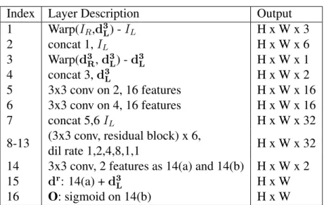
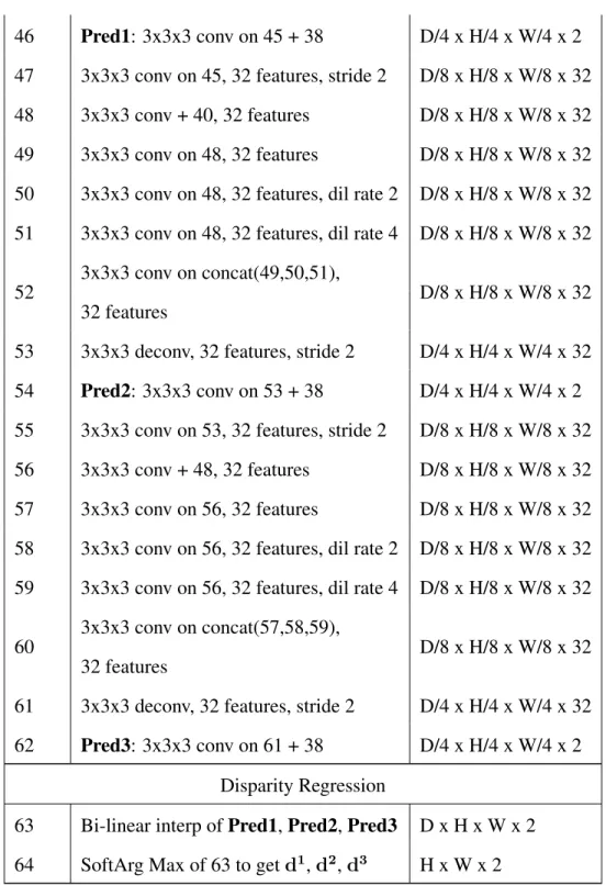
Table 3.3 – Full StereoDRNet architecture. Note that when used without refinement,

StereoDRNet just outputs

d

1

,

d

2

and

d

3

for the left view. . . 51

Table 3.4 – Quantitative comparison of the proposed Stereo-DRNet with the

state-of-the-art methods on the SceneFlow dataset. EPE represent the mean end

point error in disparity. FPS and FLOPS (needed by the convolution

lay-ers) are measured on full

960

_×

540

resolution stereo pairs. Notice even

our unrefined disparity architecture outperforms the state-of-the-art method

PSMNet (Chang and Chen, 2018) while requiring significantly less

com-putation. . . 53

Table 3.5 – Ablation study of network architecture settings on SceneFlow and

KITTI-2015 evaluation dataset. . . 53

Table 3.6 – Comparison of disparity estimation from StereoDRNet with

state-of-the-art published methods on KITTI 2012 dataset. . . 55

Table 3.7 – Comparison of disparity estimation from StereoDRNet with

state-of-the-art published methods on KITTI 2015 dataset. . . 55

Table 3.8 – Comparison of disparity estimation from StereoDRNet with

state-of-the-art published methods on ETH 3D dataset. . . 56

Table 4.1 – This table reports RMSE in 3D Reconstruction task of the proposed

Stereo-DRNet algorithm with the state-of-the-art methods in categories

includ-ing traditional multi-view stereo COLMAP (Sch¨onberger et al., 2016),

learn-ing based multi-view stereo MVSNet (Yao et al., 2018) and learnlearn-ing based

two-view stereo PSMNet (Chang and Chen, 2018). The comparison is made

on the “Sofa and cushions” scene as shown in Fig. 4.2 . . . 66

Table 5.1 –

Comparison for reconstructing shapes from the ShapeNet test set, using the Cham-fer distance. Note that due to the much smaller decoder, DeepLS is also orders

Table 5.2 –

Surface reconstruction accuracy of DeepLS and TSDF Fusion (Newcombe et al.,

2011a) on the synthetic ICL-NUIM dataset (Handa et al., 2014) benchmark

. . . 86

Table 5.3 –

Surface reconstruction accuracy of DeepLS and TSDF Fusion (Newcombe et al.,

2011a) on the synthetic ICL-NUIM dataset (Handa et al., 2014) benchmark

. . . 86

Table 5.4 –

Quantitative evaluation of DeepLS with TSDF Fusion on 3D Scene Dataset (Zhou

and Koltun, 2013). The error is measured in mm andComp(completion) corre-sponds to the percentage of ground truth surfaces that have reconstructed surfaces within7mm. Results suggest that DeepLS produces more accurate and complete 3D reconstruction in comparison to volumetric fusion methods on real depth

LIST OF FIGURES

Figure 1.1 – A simple example demonstrating a 2D-2D correspondence example that

can help to retrieve depth information of the scene. In this example, the

pixel similarity metric (absolute difference between pixel intensities) is

used as a simple correspondence function. By plotting this similarity

met-ric cost vs. increasing depth, an optimal depth value could be found that

corresponds to the local minimum. . . .

2

Figure 1.2 – An example from (Florence et al., 2018) visualizing the dense local

fea-tures in RGB color map for two soft toys in various poses. These dense

features can be used for making dense 2D-2D correspondences in

multi-views. . . .

3

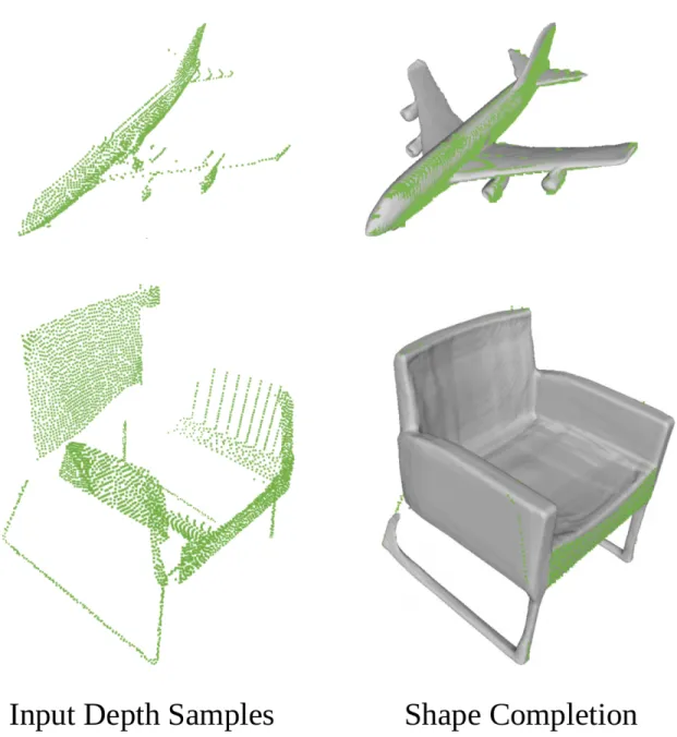
Figure 1.3 – Examples of shape competion taken from DeepSDF (Park et al., 2019).

These examples show the shape completion property of learned

implicit

surface

representation. . . .

7

Figure 2.1 – An illustration of a typical Artificial Neuron . . . 16

Figure 2.2 – Activation Functions . . . 17

Figure 2.3 – A simple Multi Layer Perceptron . . . 18

Figure 2.4 – VGG16, a convolutional neural network model proposed by (Krizhevsky

et al., 2012) for large scale image classification tasks. . . 20

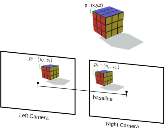
Figure 2.5 – An example showing stereo views for an object. The reference corner

point

p

(shown by green marker) of the object is viewed at different pixel

locations

p

l

and

p

r

in left and right cameras respectively. . . 24

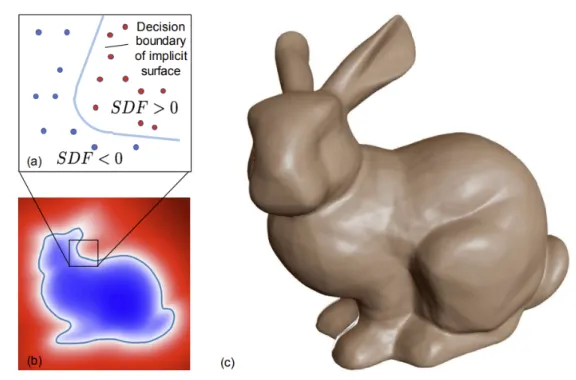
Figure 2.6 – Visualization of Signed Distance Function

f

on the Stanford Bunny 3D

model. (a) depiction of the underlying implicit surface with

SDF

=

0

on the surface contour,

SDF <

0

inside and

SDF >

0

outside the

surface boundary, (b) 2D cross-section of the signed distance field, (c)

rendered 3D surface recovered from

SDF

= 0. . . 34

Figure 3.1 – StereoDRNet network architecture pipeline. . . 42

Figure 3.2 – StereoDRNet Vortex Pooling architecture derived from (Xie et al., 2018). . . 43

Figure 3.3 – Proposed dilated cost filtering approach with residual connections. . . 43

Figure 3.5 – Disparity prediction comparison between our network (Stereo-DRNet)

and PSMNet (Chang and Chen, 2018) on the SceneFlow dataset. The top

row shows disparity and the bottom row shows the EPE map. Note how

our network is able to recover thin and small structures and at the same

times shows lower error in homogeneous regions. . . 47

Figure 3.6 – This figure shows the disparity estimation results of our StereoDRNet

and PSMNet (Chang and Chen, 2018) on the KITTI 2015 and the KITTI

2012 dataset. . . 54

Figure 3.7 – This figure shows the disparity estimation results of our refined network,

PSMNet (Chang and Chen, 2018) and DN-CSS (Ilg et al., 2018b) on the

lakeside and sandbox scenes from the ETH3D (Sch¨ops et al., 2017) two

view stereo dataset. . . 56

Figure 3.8 – This figure shows the disparity estimation results of our refined network

and several other traditional algorithms such as SGM (Hirschmuller, 2008)

and MeshStereo (Zhang et al., 2015) on three scenes from the ETH3D (Sch¨ops

et al., 2017). Notice, that StereoDRNet produces less error on object

bound-aries and maintains regularization in the prediction. . . 57

Figure 4.1 – This figure shows the proposed pipeline from input color images to

pre-dicted depth from StereoDRNet (Chabra et al., 2019) to 3D

Reconstruc-tion prepared using method described in KinectFusion (Newcombe et al.,

2011a). . . 59

Figure 4.2 – StereoDRNet enables estimation of high quality depth maps that opens

the door to high quality reconstruction by passive stereo video. In this

figure we compare the output from dense reconstruction (Newcombe

et al., 2011a) built form depth maps generated by StereoDRNet,

PSM-Net (Chang and Chen, 2018) and a structured light system (Whelan et al.,

2018) (termed Ground Truth). We report and visualize point-to-plane

dis-tance RMS error on the reconstructed meshes with respect to the ground

truth demonstrating the improvement in reconstruction over the

state-of-the-art. . . 60

Figure 4.3 – This figure shows the training scene used for all our indoor scene

recon-struction experiments. We used about 200 real stereo images in real-scene

training experiment, these views are shown in this figure by 3D axis along

with the camera trajectory visualized by the blue curve. The 3D

Figure 4.4 – We show a training example with the left image, ground truth depth and

the exclusion mask. Note that the glass, mirrors and the sharp corners

of the table are excluded from training as indicated by the yellow pixels

in the occlusion mask. Note, that this example was not part of our actual

training set. . . 62

Figure 4.5 – This figure demonstrates that our StereoDRNet network produces

bet-ter predictions on thin reflective legs of the chair and some portions of

the glass. We used occlusion mask predicted by our network to clip

oc-cluding regions. Yellow region in the ground truth are the regions that

belong to our proposed exclusion mask. . . 63

Figure 4.6 – This figure demonstrates 3D reconstruction of a living room in an

apart-ment prepared by TSDF fusion of the predicted depth maps from our

sys-tem. We visualize two views of the textured mesh and surface normals

in top and bottom rows respectively. . . 64

Figure 4.7 – Comparison of 3D reconstruction using fusion of depth maps from our

StereoDRNet network (middle), PSMNet (Chang and Chen, 2018) (right)

and depth maps from the structured light system (left) described in

(Whe-lan et al., 2018) (termed Ground Truth). We report and visualize

point-to-plane distance RMS error on the reconstructed meshes with respect

to the ground truth mesh. Dark yellow boxes represent the regions where

our reconstruction yields details that the structured light sensor or

PSM-Net were not able to capture. Light yellow boxes represent regions where

StereoDRNet outperforms PSMNet. . . 65

Figure 4.8 – This figure shows the textured 3D reconstructions of ”Sofa and cushions”,

”Plants and couch” and ”kitchen and bike” scenes developed using

Kinect-Fusion (Newcombe et al., 2011a; Whelan et al., 2018) of depth maps

gen-erated form StereoSDRNet with refinement. We visualize the camera

tra-jectory, from which the stereo images were taken, via a black curve. Note

that for clarity we visualize every 30th frame used by the fusion system. . . 66

Figure 4.9 – This figure demonstrates the surface normal visualizations of some

ob-jects (labeled with red boxes) reconstructed using

single

disparity map

from SceneFlow dataset. We report EPE in disparity space and surface

normal error in degrees. Notice, our refinement network improves the

overall structure of the objects and makes them geometrically consistent.

. . . 67

Figure 4.10 –This figure shows the surface normal visualizations of some objects

(la-beled with red boxes) reconstructed using a

single

disparity map from

our real dataset. We report EPE in disparity space and surface normal

error in degrees. Notice that our refinement network improves the

Figure 5.1 –

Reconstruction performed by our Deep Local Shapes (DeepLS) of the Burghers of Calais scene [Zhou and Koltun (2013)]. DeepLS represents surface geom-etry as a sparse set of local latent codes in a voxel grid, as shown on the right. Each code compresses a local volumetric SDF function, which is reconstructed

by an implicit neural network decoder.

. . . 70

Figure 5.2 –

2D example of DeepSDF (Park et al., 2019) and DeepLS (ours). DeepSDF

pro-vides global shape codes (left). We use the DeepSDF idea for local shape codes (center). Our approach requires a matrix of low-dimensional code vectors which in total require less storage than the global version. The gray codes are an in-dicator for empty space. The SDF to the surface is predicted using a fully-connected

network that receives the local code and coordinates as input.

. . . 77

Figure 5.3 –

Square (L∞norm) and spherical (L2norm) for the extended receptive fields

for training local codes.

. . . 79

Figure 5.4 – Instantiated local shape blocks in a scene. The blocks are allocated sparsely,

based on available depth data, which makes the approach scale well to

real world inputs. . . 80

Figure 5.5 – Interpolation in latent space of a local shape code between a flat surface

and a pole. . . 81

Figure 5.6 – This figure demonstrates how positive and negative SDF samples can be

generated for a particular depth observation. . . 82

Figure 5.7 – Fig. (a) shows the effect of changing the latent code dimensions on the

Chamfer distance test error on airplanes class of ShapeNet (Chang et al.,

2015). Fig. (b) shows an example for a scene containing

200

primitives

shapes as used for training the local shape priors. On the right side, the

instantiated local shape blocks are shown. . . 83

Figure 5.8 –

Qualitative comparison of DeepLS with DeepSDF on some shapes from the ShapeNetV2

dataset.

. . . 84

Figure 5.9 –

A comparison of the efficiency of DeepLS and DeepSDF. With DeepLS, a model

trained for one minute is capable of reconstructing the Stanford Bunny in full detail. We then trained a DeepSDF model to represent the same signed distance function corresponding to the Stanford Bunny until it reaches the same

accu-racy. This took over 8 days of GPU time (note the log scale of the plot).

. . . 85

Figure 5.10 –

Qualitative results of TSDF Fusion (Newcombe et al., 2011a) (left) and DeepLS

(right) for scene reconstruction on a synthetic ICL NUM scene. The highlighted areas indicate the ability of DeepLS to handle oblique viewing angles, partial

Figure 5.11 –

Comparison of completion (a) and surface error (b) as a function of represen-tation parameters on a synthetic scene from the ICL-NUIM (Handa et al., 2014) dataset. In contrast to TSDF Fusion, DeepLS maintains reconstruction complete-ness almost independent of compression rate. On the reconstructed surfaces (which is 50% less for TSDF Fusion) the surface error decreases for both methods (c.f. Fig. 5.12). Plot (c) shows the trend of surface error vs. mesh completion. DeepLS consistently shows higher completion at the same surface error. It scores less error than TSDF Fusion in all but the highest compression setting but it produces nearly two times more complete reconstruction than TSDF Fusion at this

com-pression rate.

. . . 87

Figure 5.12 –

Qualitative analysis of representation size with DeepLS and TSDF Fusion

(New-combe et al., 2011a) on a synthetic scene in the ICL-NUIM (Handa et al., 2014) dataset. DeepLS is able to retain details at higher compression rates (lower num-ber of parameters). It achieves these compression rates by using bigger local

shape voxels, leading to a stronger influence of the priors.

. . . 88

Figure 5.13 –

The figure shows a part of the ICL-NUIM kt0 scene (Handa et al., 2014),

re-constructed from samples with artitificial noise ofσ= 0.015. DeepLS shows better denoising properties than TSDF Fusion. For the whole ICL-NUIM bench-mark scene, DeepLS achieves a surface error of6.41mm with71.04%

com-pletion while TSDF Fusion has an error of 7.29 mm and 68.53 % comcom-pletion.

. . . 89

Figure 5.14 –

Qualitative results for DeepLS and TSDF Fusion (Newcombe et al., 2011a) on

“Burghers of Calais scene” scenes of the 3D Scene Dataset (Zhou and Koltun,

2013).

. . . 91

Figure 5.15 –

Qualitative results for DeepLS and TSDF Fusion (Newcombe et al., 2011a) on

“Lounge” scenes of the 3D Scene Dataset (Zhou and Koltun, 2013).

. . . 92

Figure 5.16 –We show qualitative comparison of DeepLS against other 3D

Reconstruc-tion techniques on a thin and incomplete dataset. We included MPU (Ohtake

et al., 2005), KinectFusion (Newcombe et al., 2011a), SSD Calakli and

Taubin (2011), PSR Kazhdan and Hoppe (2013), PFS Ummenhofer and

Brox (2015) and TSR Aroudj et al. (2017) methods in this comparison.

Notice, how most of the methods fail to build thin surfaces in this dataset.

Although, TSR fits to the thin parts but is unable to complete structures

such as the back and cylindrical legs of the stool (It fits planes to

repre-sent cylindrical legs,Fig. 5.16i). Whereas, in comparison DeepLS

recon-structs thin structures and also completes them. . . 94

Figure 5.17 –

Qualitative comparison of TSDF Fusion (left) with DeepLS (right) on real scanned

data prepared using the structured light sensor system discussed in (Straub et al., 2019a). The figure (b) is the magnified region marked with black box in figure

Figure 5.18 –

We show the scene reconstruction quality of DeepLS vs TSDF Fusion (New-combe et al., 2011a) on a partially scanned real scene dataset using the depth system described in Replica Dataset(Straub et al., 2019a). This figure shows that DeepLS provides better local shape completion than TSDF Fusion. The bottom row represents the zoomed in view marked with black box in the top

row.

. . . 96

Figure 5.19 –Completion from single-view depth images on ShapeNetV2 planes. In

both figures, the top row shows the depth image and the bottom row the

reconstructed and completed model from a different perspective. Figure

(b) shows failure cases of individual test examples that differ from the

LIST OF ABBREVIATIONS

SDF

Signed Distance Function

CHAPTER 1: INTRODUCTION

1.1

Motivation and Problem Statement

The problem of 3D Scene Reconstruction is one of the important challenges in the field of

computational photography and computer vision. The goal of this problem is to derive useful

geometric information about the environment around us. Modeling 3D environments has many

applications, such as digital mapping and navigation, virtual tourism, computer animation,

gam-ing, virtual and augmented reality (VR/AR), robot navigation. Some of these applications, such

as mapping and navigation, require accurate 3D reconstructions for precise geometry

measure-ments/estimations. Whereas some applications related to VR/AR applications require visually

pleasing, complete, and realistic 3D reconstruction to enable a feeling of presence in virtual or

augmented 3D worlds.

Many technologies and methods have been proposed to meet the needs of different

applica-tions of 3D Reconstruction. Each of these proposed methods come with their own set of strengths

and limitations. These methods can roughly be categorized into active (e.g., structured light

sen-sors and time of flight sensen-sors) and passive acquisition (using multi-view images from cameras)

techniques. Although active methods, in general, provide better scene depth information than

passive techniques, they usually require external projectors or lasers, which introduces additional

power requirements on the 3D capture system. Whereas passive techniques have the advantage of

using consumer digital cameras with low power requirements. Moreover, the prevalence and the

availability of consumer digital cameras in mobile technology widens the scope of the utility of

passive techniques in many day-to-day user applications related to 3D Reconstructions.

Figure 1.1: A simple example demonstrating a 2D-2D correspondence example that can help

to retrieve depth information of the scene. In this example, the pixel similarity metric (absolute

difference between pixel intensities) is used as a simple correspondence function. By plotting

this similarity metric cost vs. increasing depth, an optimal depth value could be found that

corresponds to the local minimum.

known as multi-view stereopsis. After decades of research in the area, the standard algorithm has

been set to estimating depth information with help of 2D-2D image correspondences, as shown

in Fig 1.1. While the standard mechanism seems very simple, solutions to many underlying

prob-lems are still not well established. For example, the optimal method for describing a good 2D-2D

correspondence function is still a challenging problem. The success of the correspondence

func-tion relies on the robustness and uniqueness of the local image descriptors. While it is simple

to obtain a strong descriptor in the regions with well-defined textures, but it is difficult to obtain

strong and unique descriptions for the regions with homogeneous texture.

Figure 1.2: An example from (Florence et al., 2018) visualizing the dense local features in RGB

color map for two soft toys in various poses. These dense features can be used for making dense

2D-2D correspondences in multi-views.

dense

image descriptors (Schmidt et al., 2016; Florence et al., 2018) as shown in Fig 1.2. These

methods use deep convolution learning framework to automatically learn robust and more general

feature descriptors with the help of known ground truth geometry of several shapes during the

training process. Unlike standard handcrafted image descriptors, these learned descriptors utilize

both local image features and global shape information. The addition of global shape information

to an image descriptor makes them robust, unique, and ideal for making dense correspondences.

The learning methods can be trained to learn descriptors for obtaining correspondences in

chal-lenging scenarios such as specular surfaces and regions with shadows. We discuss this in detail in

Chapter 3.

and how big ideally this local neighborhood should be. In general, the traditional methods in

the literature face problems defining local depth consistencies near depth discontinuities such

as corners and boundaries of the objects and thin structures like plants. Recent techniques in the

literature (Kendall et al., 2017; Chang and Chen, 2018) have tried to solve the global depth

con-sistency using a deep learning framework. By using learned convolution filters, the hard problem

of obtaining a general and robust local neighborhood depth consistency model can be solved.

Priors over local neighborhood consistencies can be learned using examples of several kinds of

shapes in the training dataset with varying thicknesses and sizes. In such frameworks, the global

scene context and semantic scene information can also be utilized. For example, the framework

can be trained to recognize pixels of an outdoor image belonging to the sky to be always at

in-finite depth. Similarly, such systems can be trained to learn priors such as walls of most of the

indoor scenes are planar. This process of learning depth cues from the scene context appears to

be similar to the human depth perception system. For example, humans can perceive approximate

scene depth with a single eye or for a single image using their knowledge of the average sizes of

individual objects and the perspective distortion. Similarly, a machine learning framework can be

trained to learn these depth cues using a variety of examples scenes during the training process.

In many applications, a depth map from a single viewpoint may not be enough to prepare a

3D reconstruction of the entire scene or an environment. A collection of depth maps from several

viewpoints should be fused together to prepare a consistent and complete 3d scene reconstruction.

The simplest 3D reconstruction representation is a collection of 3D points gathered from several

depth maps. In the literature, this representation is also known as

3D point cloud

representation.

While this representation provides accurate 3D points, it lacks surface information, which could

be useful for many applications of 3D reconstruction. In the literature, many methods have been

discussed to prepare 3D surfaces from unstructured point clouds. Most of these methods try to

formulate an

implicit surface

representation, which can be thought of as a function

F

(

p

):

, where

p

refers to any spatial point. One of the very special properties of this

implicit

func-tion

is that it is continuous, which in theory, can provide arbitrary surface resolution and has a

property of completing partially observed shapes.

In general, obtaining the true

implicit function

for an entire 3D scene is a tough problem.

Moreover, the depth samples obtained form multi-view stereo algorithms are prone to have

sev-eral kinds of noise and outliers. To make this problem tractable, the proposed methods make

several assumptions regarding the discretization of the space, noise, or uncertainty in the input

and the nature of the true surface geometry. For example, a popular method for 3D surface

re-construction (Kazhdan et al., 2006) tries to fit a global implicit function to the input set of points.

This method is shown to work very well on clean or synthetic data, but in the presence of noise,

outliers, and incomplete data, the global surface fitting is prone to produce several artifacts as no

prior information is used to predict watertight surfaces in such non-trivial cases. Scaling such

global surface fitting to large scenes also remains a challenge.

Whereas, local volumetric integration methods such as (Curless and Levoy, 1996) are more

robust to noise in the data as these methods make a scalar approximation of the true

implicit

surface

on very small cells of a regular grid. However, these methods cannot make use of the

shape completion property of the

implicit surface

representation. Moreover, such algorithms use

fixed parameters and functions to describe the region of uncertainties and fusion weights for input

samples. While this technique provides reasonable practical solutions in most cases, fixed and

heuristic functions are still prone to errors in some non-trivial cases. For example, such methods

fail to represent thin structures even at very high volumetric resolutions as the reliance on fixed

parameters and heuristic functions makes it hard to resolve both front and backside of such thin

surfaces in the presence of noise in the input samples.

representation methods reach memory limitations. Therefore, in general, the internal

implicit

surface

representation is expected to be memory efficient.

Learning

implicit surface

representation from the available ground truth shapes is an

inter-esting solution to the problems discussed above. In recent literature, some methods have been

proposed that learn the common statistics and properties of the classes of simple shapes such as

chairs, sofas. These methods take advantage of associating both the global and local shape

prop-erties to produce globally consistent 3D scene reconstructions. Majority of these methods predict

reconstructions using discrete representations such as

point clouds,

meshes

and

voxels. Like their

classical counterparts, these methods have problems related to their underlying surface

represen-tation. Very few and very recent methods, such as (Park et al., 2019), have tried to predict

implicit

surface

representation with the help of a deep learning framework. The deep learning framework

learns to separately capture both the mean and variances of the training shapes into separate

net-work parameters. In the inference process, the framenet-work utilizes the learned mean or common

properties of the trained shapes and optimizes just the variance parameters of the input shape to

fit the resultant shape to the input observations. As such methods try to learn and optimize true

implicit surface

representation, they preserve all of its properties, including shape completion

and arbitrary surface resolution without the use of any enforced assumptions and approximation,

unlike many classical approaches. We illustrate such properties in Fig 1.3.

Although, it is still challenging to express large scenes with a single true

implicit surface

representation. The authors of the work DeepSDF (Park et al., 2019) have shown the learned

implicit surface

representation of very small and simple objects such as chairs, tables, lamps,

etc. Whether such representations can be extended to large scenes efficiently still remains an

important and interesting question. In this dissertation (Chapter. 5), we try to answer this question

with a simple but promising solution.

1.

Depth estimation and 3D scene reconstruction from the input stereo images. While the

prior work in machine learning has taken long strides in solving many hard problems

re-lated to image-based 3D reconstruction and depth estimation, but still many underlying

problems need to be solved. For example, many methods in deep learning literature have

been shown to produce reasonable depth estimation from stereo images, but their depth

maps are usually not geometrically consistent enough to be fused into a consistent 3D

reconstruction. Moreover, often, the depth estimation of occluded regions is prone to be

noisy and needs to be filtered correctly before the fusion step. To tackle such problems, in

this thesis, we learn to produce occlusion aware and geometrically consistent depth

esti-mation from stereo images. Furthermore, we show that these depth images can be used to

produce 3D reconstruction of challenging indoor scenes.

meth-ods. Moreover, the resultant scene representation is still an

implicit function

and preserves

it’s properties, including shape completion and shape generation but in the scope of the

physical extent of these local shapes.

1.2

Related Work

This section starts with a summary of prior work on systems for building 3D Scene

Recon-struction using traditional methods. Next, a detailed summary of prior work is provided on

meth-ods that use machine learning for image-based 3D reconstruction. In the later section, several

methods, including learning-based depth estimation from passive images and some very recent

3D scene representation methods, are discussed.

1.2.1

3D Reconstruction using Traditional Methods

This section starts with discussing methods for obtaining depth information from general

scenes as this is the most vital requirement for any reconstruction system. Next, several

algo-rithms used in the literature for 3D scene representation are discussed.

1.2.1.1

Depth Estimation

Scene depth information can either be obtained from depth/range sensors or by using passive

stereo methods.

Active Methods

:- Traditionally, depth sensors work on the principle of Structured Light or

Time of Flight. Both these technologies are limited to work indoors and fail to work in sunlight

conditions. The range scanners such as LIDAR, etc. have low resolution and could not be used

in AR/VR based applications due to limitations in their size and resources they require. More

information on depth sensors can be found in survey (Zollh¨ofer et al., 2018).

been a lot of work in multi-view stereo based reconstruction where depth for a reference view

is obtained from many matching views. While the basic concept remains similar to two-view

stereo but having many views does not only increases the stereo search complexity but also raises

several questions related to view selection, robustness to occlusions, and geometric

consisten-cies over multiple views. A deep survey and comparisons of classical MVS based reconstruction

methods can be found in (Seitz et al., 2006). There has been a lot of work on real-time

recon-struction using passive camera motion, often known as Dense Visual SLAM (Newcombe, 2012).

These methods try to optimize for camera motion simultaneously and surface geometry

(New-combe et al., 2011b; Pradeep et al., 2013; Ummenhofer et al., 2017).

1.2.1.2

3D Scene Representation Methods

3D reconstruction using depth information has been a widely studied topic in computer vision.

The detailed state-of-the-art review can be found in the survey (Zollh¨ofer et al., 2018).

The reconstruction methods could be roughly categorized into four categories. Voxel-based

methods (Curless and Levoy, 1996; Klein and Murray, 2007; St¨uhmer et al., 2010; Newcombe

and Davison, 2010; Newcombe et al., 2011a), Points or Surfels based methods (Pfister et al.,

2000; Ummenhofer and Brox, 2013; Keller et al., 2013), Global Implicit Function approximation

methods (Carr et al., 2001; Kazhdan et al., 2006; Fuhrmann and Goesele, 2014) and Visibility or

Free Space Constraints based methods (Labatut et al., 2009; Jancosek and Pajdla, 2011; Aroudj

et al., 2017).

1.2.2

3D Reconstruction using Learning Based Methods

1.2.2.1

Learning Depth Estimation

In recent years, there has been significant improvement in the quality of depth estimation

from stereo images using machine learning techniques such as Convolution Neural Networks.

The depth maps produced by these techniques achieve much higher robustness and completion

than the previously proposed traditional methods.

The first work in this body of research, MC-CNN (Zbontar et al., 2016), proposed a siamese

neural network (Chopra et al., 2005) to compare two image patches, where the network used

the same weights while working in tandem on two different input image patches and produced a

real valued correlation between them. This learning method enabled the learning of robust stereo

cross-correlation metrics from data, which was plugged into a classical semi-global matching

process (Hirschmuller, 2008) to predict consistent disparity estimation. DispNet (Mayer et al.,

2016) improved the previous method by using an end-to-end disparity estimation deep neural

network with a correlation layer (dot product of features) for stereo volume construction. This

method enabled learning priors over the global scene context and not just the stereo-cost metric.

GC-Net (Kendall et al., 2017) improved the previous method by using high dimensional feature

vector in building stereo cost volume instead of using the dot product of feature vectors as used

in previous work. PSMNet (Chang and Chen, 2018) improved GC-Net by enriching extracted

features from CNN with a better global context using a pyramid spatial pooling process. They

also showed the effective use of residual learning networks in the cost filtering process.

Several methods such as CRL (Pang et al., 2017), iResNet (Liang et al., 2018), StereoNet (Khamis

et al., 2018) and FlowNet2 (Ilg et al., 2017) proposed depth refinement using residual learning

with guidance of photo-metric error (either in image or feature domain).

1.2.2.2

3D Scene Representation Learning

et al., 2017; Yang et al., 2017). Mesh-based methods either use existing (Sinha et al., 2016) or

learned (Groueix et al., 2018; Ben-Hamu et al., 2018) parameterization techniques to describe

3D surfaces by morphing 2D planes. Works such as (Groueix et al., 2018; Ben-Hamu et al.,

2018) use sphere parameterization to produce the closed mesh. The voxel-based method does

not usually preserve fine shape details (Wu et al., 2015; Choy et al., 2016). Octree-based

meth-ods (Tatarchenko et al., 2017; Riegler et al., 2017; H¨ane et al., 2017) alleviate the compute and

memory limitations of dense voxel methods, extending the voxel resolution up to

512

3

. Aside

from occupancy grids, a class of work (Dai et al., 2017; Zeng et al., 2017; Stutz and Geiger,

2018) extract local shape geometric descriptors from signed distance functions of local grids

(Input is SDF and output is descriptor). Unlike these methods, we extract local shape descriptors

directly from depth samples and approximate globally consistent SDF for the entire shape/scene.

More relevant to my research are the methods that approximate global implicit functions.

Occupancy Networks (Mescheder et al., 2019) tries to approximate shapes using

occupancy-based implicit function; similarly, DeepSDF (Park et al., 2019) approximates shapes using Signed

Distance Fields. Fundamentally both methods use continuous surface representation, but signed

distance fields promise better resolution with minimum computation effort. Hence we adopt

DeepSDF as the backbone architecture for my work on scene reconstruction using local shape

priors.

1.3

Thesis Contributions

corners for depth prediction while transferring learning from simulation to real scenes.

Furthermore, we demonstrate that my proposed method produces consistent 3D

reconstruc-tions even in very challenging scenes with large texture-less walls, thin structures, regions

with specular highlights, and dark shadows. This work on learning geometrically consistent

depth estimation from stereo images and subsequent fusion of the learned depth into a 3D

scene reconstruction was published as StereoDRNet (Chabra et al., 2019).

CHAPTER 2: TECHNICAL INTRODUCTION

2.1

Deep Learning for 3D Vision

The extraction of meaningful information from three-dimensional (3D) sensed data is a

fun-damental challenge in the field of computer vision. Much like with two-dimensional (2D) image

understanding, 3D understanding has greatly benefited from the current technological surge in

the field of machine learning. With applications ranging from depth sensing, mapping and

local-ization, autonomous-driving, virtual/augmented reality, and robotics, it is clear why learning of

robust functions and representation models from 3D data is in high demand. Currently, both

aca-demic and industrial organizations are undertaking extensive research to explore this very active

field further.

Classic machine learning methods such as Support Vector Machines (SVM) and Random

Forest (RF) have typically relied on a range of handcrafted shape descriptors (i.e., Local

Sur-face Patches (Chen and Bhanu, 2007), Intrinsic Shape Signatures (Zhong, 2009), Heat Kernel

Signatures (Sun et al., 2009), etc.) as feature vectors from which to learn. These methods have

delivered successful results in a range of 3D object categorization and recognition tasks.

How-ever, much like in the field of 2D image understanding, there has been a shift in focus to a deep

learning approach (LeCun et al., 2015).

for the rapid improvement in 3D understanding benchmark results, including depth estimation

and 3D reconstruction tasks.

In this chapter, we first discuss the basics of deep learning, different types of neural networks,

activation functions, and common neural network architectures. Advancement in learning depth

estimation and 3D representation learning are also discussed.

2.1.1

Deep Artificial Neural Networks

Deep Learning is a set of learning methods that attempt to model data with complex

architec-tures combining several non-linear functions. The elementary building blocks to deep learning

systems are artificial neural networks that are combined together several times to yield deep

neural networks.

An artificial neural network defines a non-linear function model

f

with respect to the model

parameters

θ

(priors) and the input

x

and the function’s output

y

can be mathematically written

as

y

=

f

(

x, θ

)

. These networks can be used to learn classification or regression tasks. These

model parameters

θ

can be estimated from learning samples. The success of such functions

was proposed in universal approximation theorem (Hornik et al., 1989). Furthermore, (LeCun

et al., 1989) introduced an efficient way to compute the gradient of neural networks using a

back-propagation algorithm.

2.1.1.1

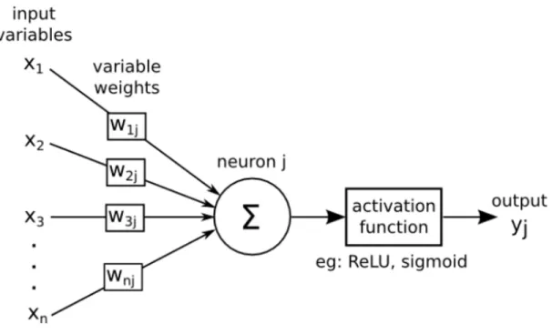
Artificial Neuron

An artificial neuron is a function

f

j

of the input

x

= (

x

1

, ..., x

d

)

weighted by a vector of

connection weights

w

j

= (

w

j1

, ..., w

jd

), completed by a neuron bias

b

j

, and associated to an

activation function

φ

, namely

y

j

=

f

j

(

x

) =

φ

(

d

X

k=0

w

jk

x

j

+

b

j

)

(2.1)

Figure 2.1: An illustration of a typical Artificial Neuron

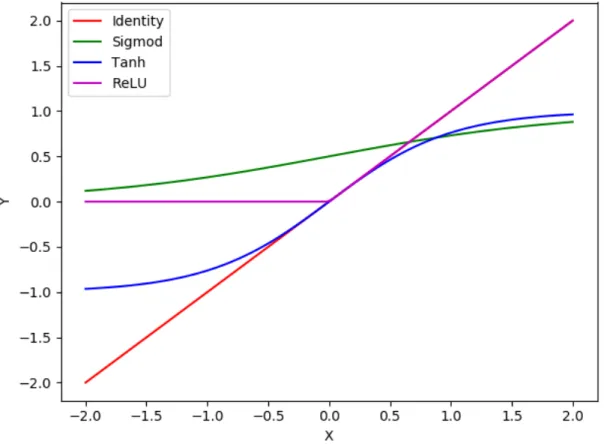
• The identity function

φ

(

x

) = 1

(2.2)

• The sigmoid function

φ

(

x

) =

1

1 +

e

−x

(2.3)

• The hyperbolic tangent function(tanh)

φ

(

x

) =

e

x

₋

_e

−x

e

x

₊

_e

−x

(2.4)

• The Rectified Linear Unit(ReLU) function

φ

(

x

) =

max

(0

, x

)

(2.5)

Figure 2.3: A simple Multi Layer Perceptron

2.1.1.2

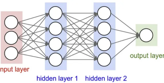
Multi Layer Perceptrons (MLP)

A multilayer perceptron is a structure composed of several hidden layers of neurons where

the output of a neuron of a layer becomes the input of a neuron of the next layer. On the output

of last layer of MLP various activation functions can be applied. The choice of the activation

depends the type of tasks to be solved by the neural network architecture. For regression tasks

typically identity or ReLU activation functions are used and for classification tasks the choice of

sigmoid activation function is generally considered.

Multilayer perceptrons are fully connected networks, i.e., each unit (or neuron) of a layer

is linked to all the neurons of the next layer. The hyper-parameters of the architecture are the

number of hidden layers and the number of neurons in each layer. An example of simple

two-layered MLP is shown in Fig 2.3

2.1.1.3

Convolutional Neural Networks

the local connectivity of the neurons. The parameters

θ

of these networks are smaller, local, and

shared. Thus, making them powerful to train than a typical MLP. Although, CNNs can only be

used when the input data is a structured grid, they have revolutionized image processing

espe-cially in tasks of learning robust features on natural images (ImageNet (Krizhevsky et al., 2012)).

A Convolutional Neural Network can be composed of several types of layers, namely

con-volution layer, pooling layer, or fully connected layer. The discrete concon-volution between two

functions

f

and

g

is defined as

(

f

_∗

g

)(

x

) =

X

t

f

(

t

)

g

(

x

+

t

)

(2.6)

For 2-dimensional signals such as images, we consider the 2D-convolutions

(

K

_∗

I

)(

i, j

) =

X

m,n

K

(

m, n

)

I

(

i

+

n, j

+

m

)

(2.7)

K

is a convolution kernel applied to a 2D signal or an image

I

. The principle of 2D convolution

is to drag a convolution kernel

K

on the image. In

convolution layers, the kernels can be used to

skip pixels defined by a number

s

, known as a stride. In each layer of CNN, zero padding can be

used to control the size of the output of the layer.

Figure 2.4: VGG16, a convolutional neural network model proposed by (Krizhevsky et al., 2012)

for large scale image classification tasks.

2.1.1.4

Optimization Algorithms

The goal is to find an optimal mapping function

f

(

x

)

to minimize the loss function of the

training samples

min

θ

1

N

N

X

j=1

L

(

y

j

, f

(

x

j

, θ

))

(2.8)

where

N

is the number of training samples,

θ

are the parameters (the weights

w

j

and biases

b

j

)

of the mapping function,

x

j

is the feature vector of the jth input sample,

y

j

is the corresponding

of stochastic gradient descent is using one sample randomly to update the gradient per iteration,

instead of directly calculating the exact value of the gradient. For detailed information on

opti-mization techniques related to machine learning we encourage readers to refer the survey (Sun

et al., 2019).

2.1.1.5

Loss Functions

Once the architecture of the network has been chosen, the parameters

θ

(the weights

w

j

and

biases

b

j

) have to be estimated from a learning sample. As usual, the estimation is obtained by

minimizing a loss function with a gradient descent algorithm. Broadly, loss functions can be

classified into two major categories depending upon the learning task we are dealing with —

Regression losses and Classification losses. In classification, we are trying to predict the output

from a set of finite categorical values i.e. Categorizing animals into different categories from a

large data set of images. Regression, on the other hand, deals with predicting real-valued

func-tions, for example, estimating scene depth, predicting prices of stocks, etc. We first discuss loss

functions that are used for classification tasks.

•

Binary Cross-Entropy Loss (BCE)

:- This is the most common setting for classification

problems. Cross-entropy loss increases as the predicted probability diverge from the actual

label. This loss function can be written

as:-L

= (

Y

)(

₋

log

( ˆ

Y

)) + (1

₋

Y

)(

₋

log

(1

₋

Y

ˆ

)

(2.9)

Where,

Y

is the ground truth label and

Y

ˆ

is the predicted label.

each category. We define Softmax function

p

i

p

i

=

e

yi

Pn

i=0

e

yi

(2.10)

The loss function is defined as

L

=

n

X

i=0

−

log

(

p

i

)

(2.11)

We now discuss several commonly used regression loss functions.

•

Mean Absolute Error (L1 Loss)

:- As the name suggests, mean absolute error is measured

as the average of the difference between predictions and actual observations. We define

MAE loss as

L

=

Pn

i=0

|

y

i

−

y

ˆ

i

|

n

(2.12)

Where,

y

i

is the ground truth value and

y

ˆ

i

is the predicted value.

•

Mean Square Error (L2 Loss)

:- As the name suggests, mean square error is measured as

the average of squared difference between predictions and actual observations. We define

MSE loss as

L

=

Pn

i=0

(

y

i

−

y

ˆ

i

)

2

n

(2.13)

Where,

y

i

is the ground truth value and

y

ˆ

i

is the predicted value.

•

Smooth L1 Loss (Huber Loss)

:- Smooth L1-loss can be interpreted as a combination of

L1-loss and L2-loss. It behaves as L1-loss when the absolute value of the argument is high,

and it behaves like L2-loss when the absolute value of the argument is close to zero. The

huber loss

H

x

equation is:

H

(

x

) =















|

x

_|

,

if

_|

x

_|

> α

x2

|α|

,

otherwise

Where,

α

is a hyper-parameter here and is usually taken as 1. The smooth L1 loss function

can now be written as

L

=

Pn

i=0

H

(

|

y

i

−

y

ˆ

i

|

)

n

(2.15)

Where

y

i

is the ground truth value, and

y

ˆ

i

is the predicted value.

2.1.2

Datasets for 3D Learning

High-quality data play a central role in enabling many computer vision technologies. For

ex-ample, the evolution of stereo algorithms greatly benefited from the Middlebury dataset (Scharstein

and Szeliski, 2003). However, the collection and labeling process of large-scale datasets for 3D

vision tasks are tedious and costly. KITTI (Geiger et al., 2012); DTU (Jensen et al., 2014), and

ETH3D (Schops et al., 2017) all require carefully calibrated camera rigs to capture images,

ex-pensive Laser scanner or structured light sensor to obtain the ground truth.

One popular way to collect training data is to utilize photo-realistic rendering engines to

synthesize large amounts of data with known ground-truth. Models trained on such synthetic

datasets demonstrated on-par or even better performances with respect to models trained on

real-world datasets. For example, SceneFlow (Mayer et al., 2016) employed rendering software to

generate data for scene flow estimation tasks.

Figure 2.5: An example showing stereo views for an object. The reference corner point

p

(shown

by green marker) of the object is viewed at different pixel locations

p

l

and

p

r

in left and right

cameras respectively.

2.2

Depth From Stereo Vision

In stereo vision, the two cameras are displaced from one another (usually horizontally) by a

fixed distance known as

baseline. This relative shift in camera geometry introduces two different

views of a scene. Due to this difference in the views of the cameras, the features captured in the

images have different locations in the stereo-images, as shown in Fig 2.6. The identification of

the difference in the location of the common features in stereo-views is known as stereo matching

[(Hartley and Zisserman, 2003)] and produces a pairing

m

(

p

l

, p

r

)

where

p

l

and

p

r

are 2D feature

locations in the left and right images respectively.

Once the pairing

m

(

p

l

, p

r

)

is obtained by the stereo-matching process, triangulation can be

stereo image pairs can be rectified to epipolar geometry. For detailed description of the process

of the stereo camera rectification, the reader is referred to (Hartley and Zisserman, 2003). For

rectified stereo-images, disparity

d

is the difference in the horizontal location between pixels

p

l

and

p

r

for the match

m

(

p

l

, p

r

). Pixels in the left and right image could be represented in image

coordinates as

p

(

u

l

, v

l

)

and

p

(

u

r

, v

r

)

respectively, the disparity

d

can be expressed as

d

=

u

l

−

u

r

.

An image

D

(

u

l

, v

l

)

where intensity values correspond to disparity

d

for each match

m

(

p

l

, p

r

)

on

the left image is known as disparity map. Disparity

d

can easily be used to estimate depth

z

using

a simple relation described in (Hartley and Zisserman, 2003) as

z

=

f

b

d

(2.16)

where

b

and

f

correspond to stereo camera baseline and focal length respectively. Estimating

these parameters of stereo camera is the part of the process known as stereo camera calibration.

2.2.1

Stereo Camera Calibration

Stereo camera calibration involves estimating both

intrinsic and extrinsic camera parameters

of the stereo camera pair.

Intrinsic camera parameters

enables practical use of the simple camera

model, transforming a 3D point in the frame of reference of the camera into a 2D point in the

camera image.

Extrinsic camera parameters

define the relative rigid geometry between two

cameras. We will now first discuss the definition of these stereo camera parameters and then

describe the calibration process.

•

Intrinsic camera parameters:- Given a point

P

(

x, y, z

)

_∈

_R

3

_{we define perspective}

projec-tion to a point

u

_∈

_R

2

as

u

=

π

(

P

)

_≡

1

where

π

is known as perspective division operator. The intrinsic calibration matrix K is

defined as:

K

_≡













f

u

0

c

u

0

f

v

c

v

0

0

1













(2.18)

with focal length

(

f

u

, f

v

)

T

and principal point

(

c

u

, c

v

)

T

. We can obtain image co-ordinates

of a projected point

p

as

p

=

Kπ

(

P

)

(2.19)

We back-project the image co-ordinates

p

, back to a point

P

using a depth

z

_∈

_R

by:

P

= (

K

−1

p

)

z

(2.20)

•

Extrinsic camera parameters:- Given a point

P

_∈

_R

3

_{in world coordinate system, this point}

can be represented in left and right camera system as

P

l

and

P

r

by

P

l

=

R

l

P

+

t

l

(2.21a)

P

r

=

R

r

P

+

t

r

(2.21b)

where

R

l

,

R

r

,

t

l

and

t

r

are rotation and translation matrices of left and right cameras. The

first Eq. 2.21a can be solved for

P

and inserted into the second Eq. 2.21b, which gives

P

r

=

R

r

R

−l 1

(

P

l

−

t

l

) +

t

r

=

R

r

R

−_l 1

(

P

l

−

t

l

+

R

l

R

−r1

t

r

)

=

R

s

(

P

l

−

t

s

)

where,

R

s

and

t

s

are relative rotation and translation matrices between the stereo cameras.

They are known as

extrinsic camera parameters

and can be written as

R

s

=

R

r

R

−l 1

(2.23a)

t

s

=

t

l

−

R

l

R

−r1

t

r

(2.23b)

We now briefly discuss the calibration process, as described in (Zhang, 2000). In this

pro-cess, typically, several images of calibration patterns are taken from various viewpoints. The

knowledge about the location of calibration points in the real world, and the image permits the

calculation of

intrinsic and extrinsic parameters

of a stereo camera pair. Zhang’s method requires

at least three images of co-planar calibration points from different positions for a unique

solu-tion. The analytic calculation uses an algebraic distance to model errors, which is only useful as

a first guess. A non-linear optimization step takes this guess and refines the values according to

the correct error model. Next, the parameters of radial lens distortion are calculated directly by

assuming that all other parameters are constant. Finally, a non-linear optimization takes place

using the full model and all parameters.

2.2.2

Stereo Matching

Approaches for solving the stereo-matching problem follow a common set of steps in order

to perform the matching

m

(

p

l

, p

r

), where

p

l

and

p

r

are 2D feature locations in the left and right

2.2.2.1

Feature Descriptors

Feature descriptors for an image are a unique set of values (or a vector) that describe useful

information. It is important that these features are easy to identify and robust under the view

changes produced by the separation of the cameras. Features can be classified according to the

information they represent as points, edges or ridges, and segments. Some of them have been

found to be robust to view-changes and have been successfully used for stereo-matching (Meltzer

and Soatto, 2008; Geiger et al., 2010). In recent work (Zbontar et al., 2016), there has been a

paradigm shift to learn these feature descriptors using machine learning approaches. We now

briefly discuss some popular handcrafted and machine-learned feature descriptors in the context

of stereo matching.