A FRAMEWORK OF RISK-BASED DECISION MAKING BY CHARACTERIZING VARIABILITY AND UNCERTAINTY PROBABILISTICALLY: USING ARSENIC
IN DRINKING WATER AS AN EXAMPLE
By
Huei-An Chu (Ann)
A dissertation submitted to the faculty of the University of North Carolina at Chapel Hill in partial fulfillment of the requirements for the degree of Doctor of Philosophy in the
Department of Environmental Sciences and Engineering.
Chapel Hill
2006
Approved By:
© 2006 Huei-An Chu (Ann)
ABSTRACT
HUEI-AN CHU: A Framework of Risk-Based Decision Making by Characterizing Variability and Uncertainty Probabilistically: Using Arsenic in Dinking Water as an Example
(Under the direction of Dr. Douglas J. Crawford-Brown)
Risk-based regulatory decisions generally apply a margin of safety meant to guard against underestimation of risk in the face of inter-subject variability and uncertainty. Since these two components often are unknown or only vaguely characterized, the decisions
involved usually employ conservative default assumptions concerning the margin of safety, resulting in regulatory limits that may be more (or less) health protective than necessary if
variability and uncertainty could be characterized probabilistically. As a result, it remains impossible in most cases to determine the degree of protectiveness inherent in a standard. The debate about maximum contaminant levels (MCLs) of arsenic is an example. At present,
we can only get a vague idea that lowering MCLs results in larger margins of safety, but at the expense of greater compliance costs. If the magnitude of this margin of safety is not taken
into account, it is possible that an MCL may be established based on a significantly larger margin of safety than is necessary, reasonable or consistent with that applied to other contaminants. Thus an unnecessarily expensive treatment policy may be selected.
In this study, a new framework of probabilistic risk-based decision making was developed. A meta-analysis was conducted for arsenic in drinking water by combining
several epidemiological studies from various regions (such as Taiwan, US, Argentina, Chile and Finland). Then the results of the meta-analysis were incorporated into the framework to
characterize the margin of safety through variability and uncertainty analyses. The final
product of this study is a method of probabilistic risk assessment that better deals with variability and uncertainty issues. This risk assessment methodology can help decision-makers make optimal determinations on regulatory limits for a contaminant that adequately
protect human health with an ample margin of safety at a more reasonable cost than currently is the case.
DEDICATION
To Jesus Christ for His Grace, the Holy Spirit for His Guidance, and God for His Glory.
ACKNOWLEGEMENTS
This dissertation could not have been done without the help and supports from others. First of all, I would like to thank my advisor, Dr. Crawford-Brown, for his guidance
and inspiring instruction on every little thing of this dissertation since the very beginning. My thanks also go to my committee members, Dr. Symons, Dr. Singer, Dr. Moreau and Dr. Characklis, for their valuable comments on this dissertation.
Then, I really appreciate the friendship and encouragement from all of my friends in these years. God used their thoughtful caring and prayers to lift me up when I am down. I
would like to share this joy with them.
I would also like to thank my Dad and Mom. Please receive my deepest gratitude and love for their dedication and the many years of support during my undergraduate and
Masters’ studies that provided the foundation for this work.
Last, but not least, I am very grateful to have my dear husband, Charles, in my life.
With his understanding, caring, companionship and love during these years, I enjoyed the whole process of my Doctoral studies and finally finished this dissertation all because of him.
Huei-An Chu (Ann)
Chapel Hill, NC, April, 2006
TABLE OF COTENTS
Page CHAPTER 1 INTRODUCTION AND STATEMENT OF THE RESEARCH
QUESTIONS ...1
1.1. Basic Statement...1
1.2. Arsenic as a Case Study...2
1.3. Study Purposes and Research Products ...4
CHAPTER 2 LITERATURE REVIEW ...6
2.1. Current Framework of Risk-Based Decision-Making ...6
2.1.1. Introduction...6
2.1.1.1. Risk ...6
2.1.1.2. Risk-Based Decision-Making in Environmental Policy ...7
2.1.2. Methodology of Risk Assessment ...9
2.1.2.1. Procedures of Quantitative Risk Assessment and the Scientific Basis...9
2.1.2.2. Risk Assessment Guidelines ...12
2.1.3. Flaws in the Current Framework of Risk-Based Decision-Making...12
2.1.3.1. Precautionary Principle...12
2.1.3.2. Unsound Scientific Basis of Risk Assessment...13
2.1.3.3. Variability and Uncertainty Issues in Risk Assessment ...14
2.1.4. Conclusion ...15
2.2. Studies on Arsenic and its Health Effects...16
2.2.1. Source, Fate and Transport of Arsenic ...16
2.2.2. Exposure Routes ...17
2.2.3. Health Effects...20
2.2.3.1. Cancerous Effects ...20
2.2.3.2. Non-cancerous Effects ...21
2.3.3.3. Blackfoot Disease in Taiwan ...22
2.2.4. Epidemiological Studies of Arsenic Exposure and Cancer Risk ...23
2.2.4.1. Epidemiological Studies in Taiwan ...24
2.2.4.2. Epidemiological Studies of Arsenic in the U.S. ...26
2.2.4.3. Epidemiological Studies of Arsenic in Other Areas ...27
2.3. Cancer Risk Assessment of Arsenic in the U.S. ...31
2.3.1. Existing Risk Assessment for Arsenic...31
2.3.1.1. Skin Cancer...31
2.3.1.2. Internal Cancers ...33
2.3.2. Variability Issues in Arsenic Risk Assessment...37
2.3.3. Uncertainty Issues in Arsenic Risk Assessment ...39
2.3.3.1. Model Choice in the Dose-Response Relationship...39
2.3.3.2. Data Limitations...42
2.3.4. Conclusion ...44
CHAPTER 3 METHODOLOGIES AND RESULTS ...45
3.1. Using Meta-Analysis in Dose-Response Assessment...46
3.1.1. Introduction of Meta-Analysis of Observational Studies ...46
3.1.2. Statistical Theory ...48
3.1.2.1. Fixed-effect model ...48
3.1.2.2. Random-effects model ...50
3.1.2.3. Calculating the Summary Estimator ...52
3.1.2.4. Test of Homogeneity...54
3.1.3. Conducting Steps ...54
3.1.4. Inorganic Arsenic in Drinking Water and Bladder Cancer: A Meta-Analysis for Dose-Response Assessment ...55
3.1.4.1. Introduction...55
3.1.4.2. Material and Methods ...56
3.1.4.3. Results...60
3.1.5. Conclusion and Discussions ...68
3.2. The Quantification of Margin of Safety...70
3.2.1. Margin of Safety and Regulatory Rationality...70
3.2.2. Reasoning for the Arsenic Case...75
3.2.3. Nested Variability/Uncertainty Analysis by Monte Carlo Simulation ...76
3.2.4. Methods...79
3.2.4.1. Variability Analysis ...79
3.2.4.2. Uncertainty analysis...81
3.2.5. Results...85
3.2.5.1. Cumulative Distribution Functions (CDFs) of Pc ...85
3.2.5.2. Fraction of Population below a Target Risk Level ...85
3.2.5.3. Confidence Analysis ...88
3.2.6. Conclusions...90
3.2.6.1. Risk Surfaces ...93
3.2.6.2. MCL Tables ...93
3.3. The Alternate Method of Quantification of Margin of Safety with Meta-Analysis Results...96
3.3.1. Methods...97
3.3.2. Results and Conclusions ...99
3.3.2.1. Confidence Analysis ...99
3.3.2.2. Risk Surfaces ...104
3.3.2.3. MCL Tables ...106
3.4. Price of Confidence...109
3.4.1. Introduction...109
3.4.2. Methods...109
3.4.3. Results and Conclusions ...112
CHAPTER 4 DISCUSSIONS ...116
4.1. Conclusions...116
4.1.1. Using Meta-Analysis in Dose-Response Assessment...117
4.1.2. The Quantification of Margin of Safety...118
4.1.3. Price of Confidence...122
4.2. Limitations, Contributions and Future Research ...124
4.2.1. Using Meta-Analysis in Dose-Response Assessment...124
4.2.2. The Quantification of Margin of Safety...125
APPENDIX A. Risk Calculation ...127
APPENDIX B. Rick Calculation using Meta-Analysis Results ...134
REFERENCES ...141
LIST OF TABLES
Table 2-1. Global Arsenic Contamination in Ground Water (Nordstrom, 2002) ...19 Table 2-2. Health Effects of Arsenic ...20 Table 2-3. Summary of US-based epidemiological studies of cancer risks from
exposure to arsenic...29 Table 2-4. Theoretical Lifetime Excess Risk (Incidence per 10,000 People) of Lung
Cancer and Bladder Cancer for U.S. Populations at Different MCLs in
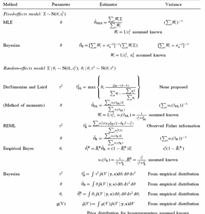
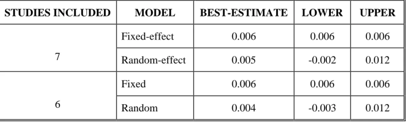
Drinking Water. ...37 Table 3-1. Summary of estimators for fixed-effects and random-effects models. ...53 Table 3-2. Studies of Bladder Cancer (188) ...59 Table 3-3. Comparison of the Results by using Different Models and including
Different Studies. ...64 Table 3-4. Risk of Bladder Cancer at different MCLs...66 Table 3-5. Steps of Reasoning ...76 Table 3-6. Results of Different Dose-response Models for Arsenic Used in the Current
Study (Showing the Difference in Predicted Values of Pc at 10 µg/L)...84 Table 3-7. Fraction of Population whose Value of Pc Exceeds the Target Value of Pc
(10 or 10 ).-4 -5 ...87 Table 3-8. The Calculated Pc from Monte Carlo Simulation at different MCLs by using
different models and their confidence, assuming the target value of F is
90%. ...88 Table 3-9. Confidence in the Claim that At Least a Fraction of the population (F) will
have Risk below the Target Value of Pc (10 or 10 ).-4 -5 ...90 Table 3-10. MCL (µg/L) at target risk of 10-5...95 Table 3-11. MCL (µg/L) at target risk of 10-4...95 Table 3-12. Arsenic Slope Factors calculated from Meta-Analysis and of other
Dose-response Models (also Showing the Difference in Predicted Values of Pc at
10 µg/L) ...96 Table 3-13. MCL (µg/L) at target risk of 10-6...107
Table 3-14. MCL (µg/L) at target risk of 10-5...108 Table 3-15. MCL (µg/L) at target risk of 10-4...108 Table 3-16. Cost (per year) Associated with MCLs. ...110 Table 3-17. Calculation of Price of Confidence (for a regulatory scenario that at least
90% of the population is below a risk of 10 )-5 ...112 Table 4-1 Comparison of MCLs (µg/L) (Given the Policy Goal that having Confidence
of 0.8 that at least 90% of the Population is Protected from the Target Risk)...122
LIST OF FIGURES
Figure 2-1. Framework of Risk-based Decision-making (NRC, 1983)...8 Figure 2-2. Components of risk assessment procedures (Moeller, 1997)...9 Figure 2-3. Dose-response relationship: linear non-threshold dose-response curve (left)
and nonlinear threshold dose-response curve (right) (Moeller, 1997)...11 Figure 2-4. Environmental Cycling of Arsenic (USEPA, 2000). ...16 Figure 3-1. The influence diagram of steps of methodologies (in blue color). ...45 Figure 3-2. Fixed-effects model. Under the assumptions of the fixed-effects model, the
expected mean of each study specific statistics, Yi, should be equal to the population mean, i.e. E (Yi) =θ. And the difference among these studies
only rest on si2= var(Yi) (Normand, 1999). ...49
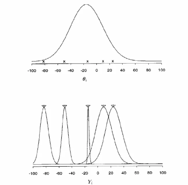
Figure 3-3. Random-effect model. Each effect, θi, is drawn from a superpopulation
with mean θ and variance τ2 (upper plot). The study-specific summary statistics, Yi, are then generated from a distribution with mean determined by
i
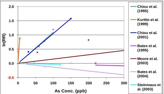
θ (denoted by × in the upper plot) and variance si2 (lower plot) (Normand, 1999). ...51 Figure 3-4. Dose-response analysis of relative risk of bladder cancer for arsenic intake
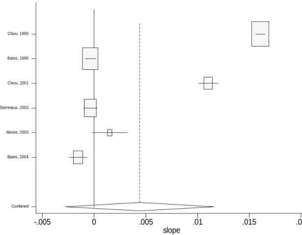
from Drinking water. ...60 Figure 3-5. Slope (with the unit of lnRR per unit increase of exposure) of each study
and the combined estimate of slope by using fix-effect model. The
horizontal line of each study corresponds to its 95% confidence interval, and the size of the square reflects the weight of each study...62 Figure 3-6. Slope (with the unit of lnRR per unit increase of exposure) of each study
and the combined estimate of slope by using random-effect model...63 Figure 3-7. Dose-response relationship of relative risk of bladder cancer for arsenic
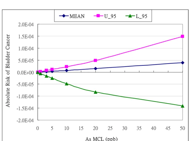
intake from Drinking water by using fixed-effect and random-effect model. ...64 Figure 3-8. Absolute Risk of Bladder Cancer at different proposed MCLs (Maximum
Contaminant Levels) from meta-analysis. (Mean: the best estimation of
slope factor, U_95: the upper bound estimation of slope factor)...66 Figure 3-9. Slope Factors of Bladder Cancer generated from Meta-analysis Results. ...67
Figure 3-10. A hypothetical relationship between MCL and the “best estimate” of risk (P) to a representative individual in the exposed population (using a linear
dose-response model)...71 Figure 3-11. A hypothetical relationship between arsenic MCL and the fraction of a
population whose risk below 10-4 (using a linear dose-response model). ...72 Figure 3-12. A hypothetical relationship between MCL and the confidence that at least
90% of the population whose risk is below 10-4 or 10-5 (in other words, no
more than 10% of the population whose risk is above 10-4 or 10-5)...73 Figure 3-13. A hypothetical surface showing the confidence (C) with which it can be
stated that at least certain fraction (F) of the population experience a risk
below a target risk (Pc). ...74 Figure 3-14. Schematic and flowchart illustrating the application of Monte Carlo
analysis to a model (Cullen and Frey, 1999). ...77 Figure 3-15. Influence Diagram for Steps of Risk Calculation employed in the study...78 Figure 3-16. Relationship between probability of cancer (x-axis) and fraction of
population below this value of Pc (F, or CDF(Pc)) under different models
and MCLs...86 Figure 3-17. Relationships between Arsenic MCLs and the fraction of population
protected from the target risk...87 Figure 3-18. CDF (Confidence) of protecting 90% of population at risk less than given
Pc and at different MCLs...89 Figure 3-19. The Confidence that at least 90% of the population whose risk is below to
the risk level (10-4 or 10-5) at different MCLs...91 Figure 3-20. The relationship between Confidence and with the fraction of population
whose risk below to the target risk level (10-4) at different MCLs. ...92 Figure 3-21. The “risk surface” showing the relationship between confidence, risk, and
the fraction of protected population to the target risk level at a given MCL...94 Figure 3-22. Risk of Bladder Cancer calculated from Different Slope Factors...97 Figure 3-23. CDF (Confidence) of protecting 90% of the population at risk less than
given Pc and at different MCLs by previous analysis and new analysis. ...100 Figure 3-24. The Confidence that at least 90% of the population whose risk is below to
the risk level (10-4, 10-5, or 10-6) at different MCLs (using meta-analysis). ...101
Figure 3-25. The Relationship between Confidence and with the fraction of the
population whose risk below to the risk level (10-6) at different MCLs...102 Figure 3-26. The relationship between Confidence and with the fraction of population
whose risk below to various risk level (10-4 and 10-5) at different MCL...103 Figure 3-27. The “risk surface” showing the relationship between confidence, risk, and
the fraction of protected population to the target risk level at a given MCL
(by the new analysis with meta-analysis). ...105 Figure 3-28. 3-D graphical presentations of the relationships among confidence, the
fraction of the population being protected at the target risk levels of 10-6(A), 10-5(B) and 10-4(C), and Costs. ...111 Figure 3-29. The Confidence of protecting 90% of population below risk of 10 and its
cost. ...113
-5
Figure 3-30. Price of Confidence (for a regulatory scenario that at least 90% of
population is below a risk of 10-5) ...113 Figure 3-31. Price of Confidence of each policy (for a regulatory scenario that at least
90% of population is below a risk of 10-5)...115
LIST OF ABBREVIATIONS
ADRI Average Daily Rate of Intake AR Absolute Risk
As Arsenic
AT Average Time
BW Body Weight
CSF Cancer Slope Factor Cw Concentration of Exposure
ED Duration of Exposure ERR Excess Relative Risk
GSD Geometric Standard Deviation
IR Intake Rate
IRIS Integrated Risk Information System
MCLs Maximum Contaminant Levels MOS Margin of Safety
NR Natural Rate
OR Odds Ratio
PDFs Probability Density Functions
RR Relative Risk
SMR Standardized Mortality Rate
95% CI 95% Confidence Intervals
CHAPTER 1INTRODUCTION AND STATEMENT OF THE RESEARCH QUESTIONS
1.1. Basic Statement
Risk-based regulatory decisions generally apply a margin of safety (MOS) meant to guard against underestimation in the face of inter-subject variability and uncertainty. Since these two components often are unknown or only vaguely characterized, the decisions
involved usually employ conservative default assumptions concerning the margin of safety, resulting in regulatory limits that may be more (or less) health protective than necessary if
variability and uncertainty could be characterized probabilistically. As a result, it remains impossible in most cases to determine the degree of protectiveness inherent in a standard. Therefore, if we had good methods of probabilistic risk assessment better dealing with
variability and uncertainty issues, we might be able to develop regulatory limits on a contaminant concentration that adequately protect human health with an ample margin of
safety at a more reasonable cost than currently is the case.
In this study, I have focused on the following general questions:
z What is the current decision-making framework used in risk-based decision-making, and what is the role of risk assessment within this framework?
z What would decisions be like under the new framework employing fully probabilistic methods?
z How can the assessment and characterization of uncertainty and variability in risk assessment be improved under the new framework?
z When variability and uncertainty are viewed probabilistically, how much does it cost to increase the margin of safety or confidence (in public health protection) when
strengthening regulatory limits on concentrations in environmental media?
1.2. Arsenic as a Case Study
I chose inorganic arsenic in drinking water as the example for my framework because “arsenic is a good example of a substance for which better scientific information is needed to
improve risk assessment needed for regulatory decisions” (Chappell et al., 1997). Ingestion of drinking water containing inorganic arsenic has become a matter of great public concern, both in the United States and globally. Inorganic arsenic in drinking water can exert toxic
effects after acute (short-term) or chronic (long-term) exposures. These health effects include cancerous effects (bladder, lung and skin cancer, and probably kidney and liver cancer) and non-cancerous effects (cardiovascular, pulmonary, immunological, neurological and endocrine such as diabetes) (NRC, 1999).
The U.S. EPA (USEPA, 2001) reconsidered its arsenic MCL (Maximum
Contaminant Level) and proposed potential MCLs of 3, 5, 10 and 20 µg/L (ppb), lowered from the original one of 50 µg/L. EPA finally proposed an enforceable MCL of 10µg/L
based on NRC reports (NRC, 1999; NRC, 2001) and application of default uncertainty
factors to provide an adequate margin of safety. This level was also determined to be
feasible technologically and economically.
However, arsenic MCLs continue to provoke scientific debate because of the variability and uncertainty issues in risk assessment. These issues include: (Frumkin and
Thun, 2001) (1) limitations in the data concerning the risk at low doses of arsenic; (2) uncertainty about the appropriate mathematical models for estimating the risk at low doses
based on data obtained from higher doses; (3) identification of any sensitive subpopulation potentially unprotected under new MCLs because of variability of health effects within the population; and (4) lack of a methodology to quantify probabilistically the margin of safety.
These controversies are actually related to each other and are associated with imperfections in the current framework of risk-based decision making. Without appropriate
models from animal studies, and because no statistical evidence of arsenic risks has been observed at levels found in U.S. drinking water systems, U.S. EPA and NRC have relied on the epidemiological data from high arsenic areas such as Taiwan (Chen et al., 1988 and 1992
and Wu et al., 1989) to estimate the risk to U.S. populations at lower arsenic levels. These data are criticized for possibly overstating the risk of arsenic ingestion in the U.S. in part
because they do not reflect differences in lifestyle, dietary habits, nutriential status and genetics. It might not be appropriate to use the Taiwanese data for the U.S. population without considering previous criticisms.
The use of a linear procedure to extrapolate from a higher, observed data range to a lower range beyond observation might also overestimate the risks. The U.S. EPA assumed
linearity for the dose-response assessments for arsenic at low doses, although some research showed that ‘when there is adequate data to characterize the mode of action, the shape of the
dose-response relationship may prove to be sub-linear below the observed range of the high
level arsenic in Taiwan’ (NRC, 1999).
Moreover, there are several sources of uncertainty and variability involving the risk assessment for arsenic in drinking water. Uncertainty results from lack of knowledge in the
underlying science. Variability comes from the differences among subjects in genetics, metabolism, diet, health status and gender. Because of the variability, some individuals or
subpopulations may be more sensitive to contaminants and have higher risks than others. Therefore, MCLs are selected to provide a margin of safety for the protection of public health even in the face of inter-subject variability and uncertainty. This margin of safety considers
factors such as inter-subject variability, quality of the database, as well as the need to extrapolate across species. However, the margin of safety is usually un-quantified; it remains
impossible in most cases to determine the degree of protectiveness inherent in a standard using a particular margin of safety (i.e. the fraction of the population protected and the degree of confidence in this protection). Taking arsenic as an example, right now we can
only get a vague idea that lower MCLs result in larger margins of safety, but at the expense of greater compliance costs. If the magnitude of this margin of safety is not taken into
account, it is possible that an MCL may be established based on a significantly larger margin of safety than is necessary, reasonable or consistent with that applied to other contaminants. Thus an unnecessarily expensive treatment policy may be selected.
1.3. Study Purposes and Research Products
The first study purpose is to incorporate meta-analysis and to improve the current dose-response assessment. The other main purpose in this study is to understand the margin
of safety for arsenic as it relates to uncertainty and variability, and to understand how an
increasing margin of safety relates to the cost of a regulation. In other words, the goal is to better characterize uncertainty and variability in risk assessment, i.e. to improve the methodology of risk assessment, focusing on the variability and uncertainty issues. My
research goal is develop a new framework of risk-based decision-making by characterizing probabilistically the variability and uncertainty in risk assessment, using arsenic as an
example.
Besides the general questions listed in the beginning, my research questions for the first study purpose include the following:
z In the observational range of available data, can meta-analysis be an appropriate tool to resolve the discrepancies among epidemiological data and get a reasonable generalized
dose-response relationship between arsenic intake and cancer risk?
z What are the uncertainty and variability distributions of risk for different MCLs of arsenic? How much confidence do we have that a given MCL will still produce
acceptable risk for a reasonable fraction of the population?
z Combining the two questions above, what is the price of this increased confidence? That is, what is the incremental cost associated with an incremental increase in the margin of safety, characterized by an increase in confidence and fraction of protected population?
The final product is a framework of risk-based decision-making to improve the
characterization of margin of safety and help to select optimal regulatory regulation limits (i.e. arsenic MCLs) that produce reasonable confidence in public health protection at
reasonable cost.
CHAPTER 2LITERATURE REVIEW
2.1. Current Framework of Risk-Based Decision-Making
2.1.1. Introduction
2.1.1.1. Risk
The definition of risk is “the probability that an individual will suffer injury, disease, or death under a specific set of circumstances” (Moeller, 1997), or the probability and
magnitude of suffering harm from any environmental problem. There are two dimensions regarding risk: (1) the probability or likelihood of the harm; (2) the severity of the harm, its magnitude or significance. The risk of concern in environmental policy is mostly from contamination of air, soil and water (Fiorino, 1995).
Generally, there are three major activities in the study of risk: (1) Risk analysis; (2)
Risk assessment and (3) Risk management. Risk analysis is the process of breaking down the concepts or ideas of a problem; for example, defining what is to be meant by the
probability of getting cancer and how confidence is to be used in estimating this probability.
Risk assessment is the step of assigning values or numbers to the concepts; for example,
calculating the specific probability of getting cancer. And risk management is the selection
2.1.1.2. Risk-Based Decision-Making in Environmental Policy
Risk assessment as well as economic analysis (cost-benefit analysis, specifically) serve as the analytical basis for environmental policy-making (Fiorino, 1995). According to Executive Order 128166 (Federal Register, 1993), it is required that all federal agencies
compare the risks of each regulatory action and provide cost-benefit analyses of the impacts of the proposed actions when developing new regulations (Moeller, 1997).
Risk assessment can be divided into the following two categories: human health risk
assessment and ecological risk assessment: The object of concern of the former one is
people and their well-being, while the object of concern of the latter one is expanded to other
animals and plants, as well as the environment itself (Fiorino, 1995).
In a summary, risk assessment is usually used in regulatory decision-making for the
following purposes (Russell and Gruber, 1987): (1) As a scientific basis
Risk assessment helps the EPA to present scientific and rational evidence for the
growing burden of proof necessary to defend its regulatory proposals in court. “Risk” also offers a scientific language by which to rationalize the regulatory decisions. With the
information from risk assessment, policy makers can select target pollutants for regulation and decide how stringently they want to control the various sources that contribute to a particular problem, and decide what actions provide “safety”; i.e., what degree of residual
risk to accept in particular circumstances. (2) Set priorities for regulation
Risk assessment helps EPA to set priorities for regulation of chemicals of potential concern and evaluate various strategies to manage risks. Quantitative risk-assessment
techniques were developed since the mid-1970s, and were used to set priorities among
pesticides, drinking water contaminants, and other toxic chemicals and to justify regulation. After setting the priorities, limited social and government resources can be directed against the most significant risks.
(3) Site-specific risk assessment
Risk assessment helps to make site-specific decisions by considering the nature of the
pollutant, the sensitivity of the environmental setting, and the availability of control questions. The most notable example of the application of risk assessment in this context is the Superfund Program.
The current framework of risk-based decision-making is shown in Figure 2-1.
Figure 2-1.Framework of Risk-based Decision-making (NRC, 1983).
2.1.2. Methodology of Risk Assessment
Risk can be expressed qualitatively or quantitatively. An example of the former is
EPA’s five categories for toxic agent (A - E), assigned depending on an agent’s potential for causing cancer in humans. Arsenic has been categorized in list A, which is “known to be human carcinogens” (Frumkin and Thun, 2001). Risk can also be expressed quantitatively;
for example, probabilistic risk assessment expresses risk as a probability ranging from zero (certainty that harm will not occur) to one (certainty that harm will occur) (Moeller, 1997).
This research focused on quantitative risk assessment.
2.1.2.1. Procedures of Quantitative Risk Assessment and the Scientific Basis
The four procedures of quantitative risk assessment and the scientific basis are explained in the following paragraphs and summarized in Figure 2-2 (NRC, 1983).
Figure 2-2. Components of risk assessment procedures (Moeller, 1997).
(1) Hazard identification
This procedure produces a qualitative judgment as to whether an agent has any potential to cause adverse health effects following exposure. The question asked in this step, for example, is “does arsenic cause adverse health problems in humans through drinking
water?” The evidence can usually be derived from four general classes of information, including epidemiological data, animal-bioassay data, short-term in vitro assays, and
comparisons of molecular structure. Their importance in estimating risk to humans is in roughly decreasing order. (Crawford-Brown, 1999) The EPA’s integrated risk information system (IRIS) can be a source for information about the potential toxicity of an agent.
(2) Exposure assessment
This procedure identifies populations exposed to the toxicant, describes their composition and size, and examines the routes, magnitudes, frequencies, and durations of such exposures. Example questions in this procedure are: “what is the concentration of
arsenic in groundwater?” and “what are the major exposure pathways of arsenic to human populations?”
The first task in this step is to determine the concentration of the chemical to which humans are exposed. This may be done by direct measurement or by a model if exposure data are incomplete or cannot be obtained directly. The second task is to determine which
group in the population may be exposed and if there is any subgroup in the population which is more susceptible to the exposure. In the situation of exposure to a mixture of carcinogens,
if data are unavailable, synergistic effects are often ignored or accounted for by the use of various safety factors.
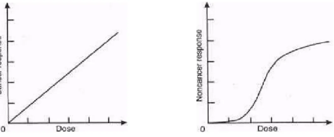
(3) Dose-response assessment
This procedure estimates the relationship between dose and response quantitatively. The estimation can be based on epidemiological observations, animal data, or studies of mechanisms of action. A typical question is: “what is the relationship between arsenic intake
(dose) and incidence of cancer?” Figure 2-2 presents two possible dose-response curves. If useful human data are absent, a model for animal-to-human dose extrapolation will be used.
If available data (epidemiological or animal) are only available at high dose, a model for low-dose extrapolation will be used.
Figure 2-3. Dose-response relationship: linear non-threshold dose-response curve (left) and nonlinear threshold dose-response curve (right)(Moeller, 1997).
(4) Risk characterization
This procedure presents the policy-maker with an overall conclusion about the magnitude of risk, the variability of risk in the exposed population, and confidence in estimates of risk. The assumptions underlying the assessment of uncertainty are also
provided in this step.
2.1.2.2. Risk Assessment Guidelines
To avoid inconsistent assumptions and value judgments by different programs within the EPA, several Risk Assessment Guidelines have been provided as a consistent approach across programs. The functions of this kind of guideline include informing EPA risk
assessors on the best available science and risk assessment techniques, establishing a standard for quality of work and comparison of studies,providing for consistency and orderly
decision-making, helping inform the public about how scientific judgments and assumptions have been incorporated into risk assessments, and helping show where additional research and analysis might be necessary. In a word, they can provide EPA staff and decision makers
with guidance for developing and using risk assessments, and provide basic information to the public about the Agency’s risk assessment methods. However, this kind of guideline is
not an official regulation, and represents neither a perfect methodology nor an ideal consensus among scientists (USEPA, 1996; USEPA, 1999; USEPA, 2003).
2.1.3. Flaws in the Current Framework of Risk-Based Decision-Making
2.1.3.1. Precautionary Principle
One of the critiques of the current risk assessment framework is that it is overly conservative due to the precautionary principle. The definition of the precautionary principle is: “when information about potential risks is incomplete, base decisions about the best way
to manage or reduce risks on a preference for avoiding unnecessary health risks instead of unnecessary economic expenditures”. Based on this “better to be safe than sorry” principle,
the most conservative models and assumptions are usually selected for use in risk assessment,
and EPA usually selects an MCL or regulatory limit to provide a large margin of safety
(MOS) for the protection of public health to reflect the quality of the database, inter-subject variability and uncertainty; as a result, the compliance cost may be high.
2.1.3.2. Unsound Scientific Basis of Risk Assessment
Another critique is that risk assessment may not provide sound/good science for
environmental policy because of uncertainty and variability factors. An NRC report (NCR, 1994) listed the following potential flaws in the scientific bases for risk assessment:
(1) Default assumptions adopted when evidence is not sufficient may have been unduly
conservative.
(2) Default options may have become too rigid, with an unnecessarily large barrier to the
adoption of new, more scientifically defensible, assumptions.
(3) Aspects of risk established as significant in science (e.g. synergisms/antagonisms) are missing from the risk assessment process.
(4) Uncertainties in risk estimates are inadequately described and knowledge may have been insufficient to justify quantifying risk.
(5) Risk estimates obtained under conservative assumptions for screening may have been applied to final, risk-based, decisions.
(6) Results of risk assessments may have been given too little, or too much, weight of
decisions.
In a word, the default assumptions and extrapolation methodology (i.e. linearity
assumption in low-dose extrapolation) used in EPA’s risk assessments have been criticized
based on the claim that they are unsupported scientifically, raise needless public fears and
waste money on costly and unnecessary protective measures.
2.1.3.3. Variability and Uncertainty Issues in Risk Assessment
Another flaw of the conventional framework of risk-based decision making is the inability to characterize the variability and uncertainty well. “Variability means the
distribution of some real quantity among things or people even after the application of perfect measurement techniques, whereas uncertainty is a description of the imperfection of our information about a parameter (including a parameter describing real variability)” or lack of
knowledge in the underlying science (Hattis et al., 1999). For example, inter-subject variations in factors contributing to risk may include genetics, metabolism, diet, health status,
nutrition, gender, and other possible factors, whereas uncertainty may result from model choice.
Considering variability and uncertainty issues in risk assessment, regulatory policy
has to apply a “Margin of Safety” as part of regulatory rationality. In other words, margins of safety are generally applied to guard against underestimation in the face of inter-subject
variability and uncertainty. Therefore, regulatory decisions usually employ conservative default assumptions to guard against inadequate margin of safety in the face of variability and uncertainty. This may result in regulatory limits that may be more (or less) health
protective than necessary. And this also leads to criticism about the margin of safety because it is impossible to estimate the magnitude of that margin.
2.1.4. Conclusion
Considering these flaws in the current framework, arsenic in drinking water may be a
good case study to improve the risk assessment methodology and the whole risk-based regulatory decision-making (Chappell et al., 1997). The controversies in the arsenic case are due to imperfections in the current framework of risk-based decision making. If the
problems in arsenic case can be examined in detail and solved, these should contribute to a better risk assessment methodology needed for regulatory decisions. More specifically, if we
had good methods of probabilistic risk assessment better dealing with variability and uncertainty issues, we could develop regulatory limits on a contaminant concentration that adequately protect human health with an ample margin of safety at a more reasonable cost
than currently is the case. Details regarding the issue of arsenic in drinking water will be addressed in the following sections.
2.2. Studies on Arsenic and its Health Effects
2.2.1. Source, Fate and Transport of Arsenic
Arsenic and its compounds are mobile in the environment. Water is the primary
medium for arsenic transport in the environment (Pontius et al., 1994). The pentavalent species (As5+, arsenate) is the predominant compound; trivalent arsenic (As3+, arsenite) is only found under anaerobic conditions (NRC, 1999). The cycling of arsenic in the
environment is presented in Figure 2-4 (USEPA, 2000).
Figure 2-4. Environmental Cycling of Arsenic(USEPA, 2000).
Although arsenic is released to the environment from both natural and anthropogenic
sources, most arsenic is naturally occurring in the environment in both inorganic and organic forms. The major natural source of arsenic is from the erosion, dissolution or weathering of arsenic-containing minerals, rocks or soils; the dissolved arsenic enters groundwater or
surface water. Other natural sources include volcanic eruption and forest fires. Anthropogenic sources are from industrial processes, such as mining, smelting, wood
preserving, pesticide spraying and coal burning (USEPA, 2000).
2.2.2. Exposure Routes
Humans are exposed to various forms of arsenic with different toxicities. The
metallic form of arsenic (0 valence) has not been shown to be associated with any adverse effects; a volatile compound such as arsine (AsH3) is toxic, but is not contained in water or
food; organic forms of arsenic (primary arsenobetaine and arsenocholine), which can be found in fish and shellfish, have little or no toxicity; inorganic arsenic, i.e. arsenite (As3+) and arsenate (As5+), are the most prevalent toxic forms found in drinking water, and have been
reported to be more toxic than the organic ones. Moreover, the trivalent form (+3) is more toxic than the pentavalent one (+5) (USEPA, 2001).
Inhalation of air, food intake and ingestion of water are the major routes for humans
to be exposed to arsenic. Among these routes, drinking water and food are the most significant ones; only a relatively small amount of arsenic is inhaled. Other routes, such as
absorption of arsenic through the skin or ingestion of arsenic-containing soils or dust are possible but thought to be insignificant (Pontius et al., 1994; Abernathy et al., 1996; Abernathy et al., 2003).
Occupational exposure is the major cause of arsenic inhalation, such as workers who
manufacture arsenical pesticides or work in mines and copper smelters (Frumkin and Thun, 2001). Besides occupational inhalation, air mostly represents a minor source of exposure for the general population (Buchet and Lison, 2000).
As for non-occupational exposure, drinking water and food are the major sources (Borum and Abernathy, 1994). Dietary intake is a significant source of arsenic. Food such
as seafood, fruits and vegetables contain organic arsenic. About half of the dietary intakes come from seafood, such as fish and shellfish, followed by meat and poultry, grain and grain products, and vegetables. Infants and toddlers also get arsenic through their diet from milk
and milk products. However, most adverse health effects of arsenic are from drinking water rather than food, because most food arsenicals are organic. Organic arsenic in food is less
toxic than inorganic forms and most can be excreted rapidly (Pontius et al., 1994; Abernathy et al., 2003). But the dietary contribution to daily intake of arsenic may become dominant if arsenic intake through drinking water is at low concentrations (Hering, 1996).
Ingestion of arsenic through drinking water is the major concern of arsenic exposure. Arsenic concentration is generally higher in groundwater than in surface water, especially
high in places where geochemical conditions favor arsenic dissolution (Pontius et al., 1994). Table 2-1 lists the global arsenic contamination in ground water (Nordstrom, 2002). And the following regions have been found to be geological strata naturally rich in arsenic: Taiwan,
West Bengal, Mexico, Chile, Argentina, Mongolia, Finland, Hungary and the western and southwestern states and Alaska of the US (Chappell et al., 1997; Thornton and Farago, 1997).
In these regions, the natural arsenic concentration may reach levels up to several hundreds of µg/L or even a few mg/L (Buchet and Lison, 2000). About 98% of the U.S. population uses
drinking water with concentrations less than 10 µg/L. But some portion of the remaining 2%
of the population is exposed to arsenic concentrations that may reach 50-100 µg/L (Chappell et al., 1997).
Table 2-1. Global Arsenic Contamination in Ground Water (Nordstrom, 2002)
Country/Region
Potential Exposed Population
Concentration
(µg/liter) Environmental Conditions
Bangladesh 30,000,000 <1 to 2,500 Natural; alluvial/deltaic sediments with high phosphate, organics
West Bengal,
India 6,000,000 <10 to 3,200 Similar to Bangladesh Vietnam >1,000,000 1 to 3,050 Natural; alluvial sediments
Thailand 15,000 1 to >5,000 Anthropogenic; mining and dredged alluvium
Taiwan 100,000 to
200,000 10 to 1,820 Natural; coastal zones, black shales Inner Mongolia 100,000 to
600,000 <1 to 2,400
Natural; alluvial and lake sediments; high alkalinity
Xinjiang, Shanxi >500 40 to 750 Natural; alluvial sediments
Argentina 2,000,000 >1 to 9,900 Natural; loess and volcanic rocks, thermal springs; high alkalinity
Chile 400,000 100 to 1,000
Natural and anthropogenic volcanogenic sediments; closed basin; lakes, thermal springs, mining
Bolivia 50,000 - Natural; similar to Chile and parts of Argentina
Brazil - 0.4 to 350 Gold mining
Mexico 400,000 8 to 620 Natural and anthropogenic; volcanic sediments, mining
Germany - <10 to 150 Natural: mineralized sandstone Hungary,
Romania 400,000 <2 to 176 Natural; alluvial sediments; organics Spain >50,000 <1 to 100 Natural; alluvial sediments
Greece 150,000 - Natural and anthropogenic; thermal
springs and mining
United Kingdom - <1 to 80 Mining; southwest England
Ghana <100,000 <1 to 175 Anthropogenic and natural; gold mining
USA and
Canada - <1 to >100,000
Natural and anthropogenic; mining, pesticides, As2O3 stockpiles, thermal
springs, alluvial, closed basin lakes, various rocks
2.2.3. Health Effects
As mentioned previously, inorganic arsenic is considered to be significantly more
toxic than the organic form. Thus exposure to organic arsenic is usually not considered in assessing health risks (Hering, 1996). Inorganic arsenic (hereafter called arsenic) in drinking water can exert toxic effects after acute (short-term) or chronic (long-term) exposures (NRC,
1999). The health effects caused by arsenic are positively correlated with the dose and duration of exposure (NRC, 2001), and are classified in Table 2-2.
Table 2-2. Health Effects of Arsenic
Health Effects Symptoms References
Acute toxicity
Gastrointestinal irritation accompanied by difficulty in swallowing, thirst, abnormally low blood pressure, and convulsions.
Death because of cardiovascular collapse.
(Pontius et al., 1994)
Chronic non-cancerous effects
Dermal changes, such as skin pigments, hyperkeratosis, and ulcerations.
Vascular effects, such as blackfoot disease
Cardiovascular, pulmonary, immunological, neurological and endocrine (e.g., diabetes) effects.
(Pontius et al., 1994)
(NRC, 1999)
Chronic cancerous effects
Skin cancer
Internal cancers, such as bladder, lung, and liver cancer. The evidences for other cancers, such as kidney, nasal passages, prostate, and other internal sites cancer are not strong.
(NRC, 1999)
2.2.3.1. Cancerous Effects
Ingestion of inorganic arsenic may have chronic cancerous effects. The 1999 NRC report confirmed that arsenic in drinking water causes bladder, lung and skin cancer, and might cause kidney and liver cancer. Skin cancer has been established as a health effect.
However, skin cancer is not as great a concern as other internal cancers because internal
cancers are life threatening but most skin cancers are not (NRC, 2001).
The evidence for lung and urinary bladder cancers has been strengthened by recent studies in Taiwan, Argentina, and Chile. But most of these epidemiological studies for
cancer were from areas with relatively high arsenic concentration (at least several hundred micrograms per liter, which is much higher than the average concentration in the U.S.).
Cancer risk at lower concentrations of ingested arsenic, however, has been seldom addressed in such studies. Other cancers, such as kidney and liver cancer, have also been found to have an association with ingestion of inorganic arsenic. Nevertheless, their association is not
strong enough to allow reliable identification of increased risk in existing studies. Therefore, further confirmatory studies are needed to establish arsenic as a cause of cancers other than
skin, lung and bladder cancers (NRC, 1999).
2.2.3.2. Non-cancerous Effects
Ingestion of inorganic arsenic may also have chronic non-cancerous effects on multiple-organ systems. These effects are dependent on the magnitude of the dose and the
time course of exposure. The toxicokinetic and toxicodynamic interaction between the dose and exposure time has still not been well characterized. From the available data, some general findings have emerged, such as hypertension and diabetes, although the NRC found
the relationship still unquantifiable. Effects noted by the NRC include (NRC, 1999):
(1) Nonmalignant dermal effects, such as diffuse or spotted hyperpigmentation and
palmar-plantar hyperkeratoses.
(2) Obvious nonspecific gastrointestinal complaints, such as diarrhea or cramping.
(3) Hematological effects, such as anemia and leukopenia.
(4) Neurological effects, such as a sensory predominant axonal peripheral neuropathy.
(5) Cardiovascular effects, such as irreversible noncirrhotic portal hypertension and cardiovascular mortality.
(6) Peripheral vascular disease, such as Blackfoot disease.
(7) Cerebrovascular disease, but the evidence for this effect is not clear.
(8) Diabetes (diabetes mellitus).
(9) Immune function effects, but these effects have not been adequately studied in field research.
(10) Respiratory effects, but the specific pathology of this effect has not been investigated. (11)Reproductive and development effects. Arsenic may be teratogen and can cause
stillbirth, increase of infant mortality, preterm births, or spontaneous abortions.
2.3.3.3. Blackfoot Disease in Taiwan
Blackfoot disease is a peripheral vascular disease and has been endemic in a small area on the southwest coast of Taiwan since 1954. Disease symptoms start with spotted
discoloration of the skin of extremities, especially the foot. The spots change from white to brown, then to black. Affected skin gradually thickens, cracks, and ulcerates (Tseng et al., 1968). A considerable percentage of patients suffered from great pain and even tried to
commit suicide because the pain was intolerable. Some of them finally had to cut their affected extremities. This has caused much inconvenience and difficulty in daily lives and
social problems. It has been found that the prevalence of Blackfoot disease was related to the ingestion of water from deep wells with high arsenic concentration.
People who have lived in villages along the southwest coast have used artesian well
water with high concentration of arsenic since the 1900s. Artesian well water was no longer used during the mid-1970s because the tap-water system had been gradually installed since 1956. The government also persuaded residents not to drink arsenic-containing well water or
groundwater. As time went by, the Blackfoot disease cases decreased gradually and were almost eliminated. However, 40 years later in 1996, about 20 people got a similar disease in
the northeast area of Taiwan. The groundwater in this area also contains high concentrations of arsenic (Chiou et al., 2001). The fact that Blackfoot disease was prevalent in the areas with high arsenic concentration in groundwater has been noted, and substantial studies have
been done in Taiwan.
2.2.4. Epidemiological Studies of Arsenic Exposure and Cancer Risk
Inorganic arsenic is not typically found to cause tumors in standard laboratory animal tests, while the observational studies of human exposures to arsenic through ingestion have been strongly associated with increases in skin and internal cancers (Clewell et al., 1999).
Still, the association between arsenic exposure and cancerous effects is controversial and not well established in the epidemiological field. Varied or even opposite results have been found in different epidemiological studies of different regions. Some studies (e.g. studies in
Taiwan) showed significantly elevated incidence or mortality of cancers for the population exposed to arsenic, while some others (e.g. studies in the US) failed to show an association
between arsenic in drinking and the adverse health effects.
2.2.4.1. Epidemiological Studies in Taiwan
Since 1968, researchers in Taiwan kept finding that populations in these Blackfoot-endemic areas also had high rates of some cancers, such as skin, bladder, kidney, liver, and lung cancer (Tseng et al., 1968; Tseng, 1977; Chen et al., 1985; Chen et al., 1988; Wu et al.,
1989; Chen and Wang, 1990; Chen et al., 1995; Chen et al., 1996; Chiou et al., 1997; Hsu et al., 1997; Hsueh et al., 1997; Tsai et al., 1998; Tsai et al., 1999). Most of these
epidemiological studies showed that there was a significantly elevated incidence of cancers for the study population (which is confined in the Blackfoot disease endemic area) compared with lesser-exposed populations in both communities with similar socio-economic structure
as well as with the general population in Taiwan. Some studies also showed dose-response relationships with increasing arsenic concentrations (NRC, 1999). Chappell et al. (1997) remarked on the possible shortcomings of these studies, noting that “these studies from Taiwan demonstrate a dose-response relationship for cancer at various sites and arsenic concentrations in water, but the data are not sufficiently precise for accurate quantitative
assessment of the magnitude of cancer risk at different arsenic concentrations needed to set an MCL in the United States because the studies report exposures for groups of people rather
than for individuals” (Chappell et al., 1997).
The two prevalence studies of skin cancer conducted by Tseng and his colleagues (Tseng et al., 1968; Tseng, 1977) were recognized as the best available data for EPA to
conduct quantitative risk assessment (USEPA, 1984; USEPA, 1988). However, the shortcomings of these studies are that the exposure categories are too broad and too few:
There were only three defined exposure categories (0-290 µg/L, 300-590 µg/L, 600 µg/L and above, and undetermined) and the upper limit of the lowest exposure category was quite high
(290µg/L). Another shortcoming is that these studies were ecological in design and the data
were analyzed by using all residents in a given village instead of an individual as a unit (Guo and Valberg, 1997). Chen and his colleagues did another important epidemiological study (Chen et al., 1985; Chen et al., 1988). They studied the same regions as Tseng et al. did, but
used mortality data. They found an increased occurrence of cancer in internal organs, including bladder, liver, lung and other sites. Their studies had similar shortcomings with the
ones of Tseng el al. with respect to exposure grouping and ecological study design. U.S. EPA (USEPA, 1988) used the Tseng study data to conduct a dose-response assessment for skin cancer, while Smith el al. (Smith et al., 1992) used the Chen study data to conduct a
dose-response assessment for internal cancers (bladder, liver, lung, kidney) (Brown et al., 1997).
While most of the previous Taiwanese studies were conducted in an area with relatively high arsenic concentration (200 ppb or more), recent studies have discovered that low-dose exposure to arsenic may also increase the risk of certain types of cancer, diabetes
and vascular disease. This study conducted by Chiou et al (2001) examined cases of urinary tract cancer in villagers exposed to arsenic levels as low as 10 to 50 ppb. His research
concluded that there was a significantly increased incidence of urinary cancers for the study cohort compared with the general population in Taiwan, even at low arsenic concentration. This study had a better study design that estimated arsenic exposure at an individual level
(i.e., based on the arsenic concentration in his or her own well water), making the study result more reliable (Chiou et al., 2001). Also, this study and the one done in Chile (Ferreccio et al.,
2000) were said to “have adequate data to contribute to quantitative assessment of risk” in NRC’s arsenic report in 2001 (NRC, 2001).
2.2.4.2. Epidemiological Studies of Arsenic in the U.S.
Despite there being substantial studies outside the U.S., it is still unclear whether arsenic in drinking water occurring at environmental levels leads to adverse health effects in the U.S.
Early US studies (Goldsmith et al., 1972; Morton et al., 1976; Harrington et al., 1978; Southwick et al., 1983; Valentine et al., 1985) in communities with high arsenic levels in
water supplies have failed to show an association between arsenic in drinking water and adverse health effects. However, Bates el al. (1992) pointed out that “these studies have had cross-sectional designs, and the exposed populations have been small, probably relatively
mobile and with access to alternative water sources” (Bates et al., 1992). These factors generated statistical power too low to detect effects (Pontius et al., 1994). Other
epidemiological studies (Valberg et al., 1998) showed the same results of health effects in high-arsenic regions; i.e. no association between skin-cancer prevalence and arsenic in drinking water was found. This result could be due to an absence of risk in the U.S.
populations or statistical limitations due to small sample sizes (Chappell et al., 1997).
More recently, the Utah Study (Lewis et al., 1999) did not find any excess bladder or
lung cancer risk with exposure to arsenic at concentrations from 14 to 166 µg/L. They estimated excess risk by comparing cancer rates among the study population, in Millard County, Utah to background rates in all of Utah, and the result showed that there are
important differences between the study and comparison populations besides their consumption of arsenic. One explanation for such a difference is that Millard County is
mostly rural, while Utah as a whole contains some large urban populations. Another explanation is that the subjects of the Utah study were all members of the Church of Jesus
Christ of Latter Day Saints, who for religious reasons have relatively low rates of tobacco
and alcohol use. Therefore, this study was criticized in that “the comparison of the study population to all of Utah is not appropriate for estimating excess risks” (USEPA, 2001). The Agency (USEPA, 2000) reanalyzed the Utah data by an alternative method of comparing
cancer rates only among people within the study population who had high and low exposures. The results showed that there was still no detectable increased risk of lung or bladder cancers
due to arsenic, even among subjects exposed to more than 100 µg/L on average”. And the EPA finally concluded: “The Utah study is not powerful enough to estimate excess risks with enough precision to be useful for the Agency’s arsenic risk analysis” (USEPA, 2001).
Karagas and his colleagues (2001) conducted a case-control study to investigate the relationship between skin cancer risk and arsenic exposure in New Hampshire. They used
toenail arsenic concentrations as a biological marker of arsenic exposure through drinking water. While the risks did not appear elevated at the toenail arsenic concentrations detected in most study subjects, the authors could not exclude the possibility of a dose-related increase
at the highest levels of exposure experienced in the New Hampshire population (Karagas et al., 2000; Karagas et al., 2001). Schoen et al. (2004) summarized epidemiological studies in
the U.S. in the following Table 3 (Schoen et al., 2004).
2.2.4.3. Epidemiological Studies of Arsenic in Other Areas
Results of arsenic studies in other areas have been mixed. An association was found between bladder cancer mortality and arsenic in drinking water in Argentina
(Hopenhayn-Rich et al., 1996). They also found that arsenic ingestion increases the risk oflung and kidney cancers, but the association between arsenic andmortality from liver and skin cancers
was not clear in another study (Hopenhayn-Rich et al., 1998). Another case-control study in
Argentina done by Bates et al. (2004) found increased bladder cancer risks associatedwith high levels of arsenic in drinking water, but little informationexists about risks at lower concentrations. This study suggests lower bladder cancer risksfor arsenic than predicted
from other studies, but the authors add that the latency for arsenic-induced bladder cancers may belonger than previously thought (Bates et al., 2004).
Kurttio et al. (1999) studied the association of arsenic exposure from drilled well water with the risk of bladder and kidney cancers in Finland. In spite of very low exposure levels, some evidence of an association between arsenic and bladder cancer risk was found.
But none of the exposure indicators was statistically significant in the association with the risk of kidney cancer (Kurttio et al., 1999).
Increased mortality in bladder and lung cancers were found in a region of northern Chile (Smith et al., 1998). Ferreccio et al. (2000) conducted a case-control study in cities in northern Chile where arsenic concentration was 860 µg/L in drinking water in the period
1958–1970 and reduced to 40 µg/L since then. They investigated the relation between lung cancer and arsenic in drinking water over time. Strong evidence has been shown that
ingestion of inorganic arsenic is associated with lung cancer (Ferreccio et al., 2000). Due to many strengths of this study, the data from this study were evaluated to be useful in further quantitative risk assessment (NRC, 2001).
A complete list and summary of current major epidemiological studies from different regions, in which cancers are the end points to be investigated, are presented in NRC reports
(NRC, 1999; NRC, 2001). Please see Tables 2-3 for details (Schoen et al., 2004).
Table 2-3. Summary of US-based
epidemiological studies
of cancer
risks from ex
posure to a
rsenic
(Schoen et al., 2004).
Table 2-3. Summary of US-based epidemiological studies of cancer risks from exposure to arsenic.
2.3. Cancer Risk Assessment of Arsenic in the U.S.
2.3.1. Existing Risk Assessment for Arsenic
Cancer risk has been the driving effect in regulatory decisions because non-cancer effects are likely to be significant only at concentrations well above the considered MCLs
(USEPA, 2001). Therefore, the discussion about arsenic risk assessment in this chapter is focused on cancer.
Most arsenic cancer risk assessments have been based on epidemiological studies. In
the United States, the risk assessments of arsenic from drinking water were at first done for skin cancer. And it was agreed that ingested arsenic causes enhanced skin cancer risk. Then,
several risk assessments were done for internal organ cancers (lung, liver, kidney, bladder) from drinking arsenic-rich water, and it was also shown to cause increased risk in these end points. However, because of uncertainty and variability issues in risk assessment, there have
been several debates about the validity of these risk assessments.
2.3.1.1. Skin Cancer
The U.S. EPA (1984, 1988) conducted a risk assessment for skin cancer by using data from southwestern Taiwan where Blackfoot disease is endemic (Tseng et al., 1968; Tseng,
1977). The EPA used the “cancer slope factor” (CSF) or the “cancer potency factor” as an estimation of carcinogenic potency and assumed a linear dose-response relationship (USEPA, 1988; Brown, 1998). The upper-bound excess cancer risk from lifetime exposure to water
containing 1 µg As per liter (unit risk) was calculated to equal to 5 ×10⁻⁵ by using a generalized multistage model. Consuming drinking water at the MCL of 50 µg/L (which was
the MCL of arsenic at that time) entailed a lifetime risk of 2.5 ×10⁻³. However, the unit risk
calculated by the EPA could overestimate the actual risk for skin cancer. That is because the
EPA extrapolated data from Taiwan with high-level arsenic exposures linearly to generate risk estimates for low-level exposures in the U.S. For this extrapolation, the EPA hypothesized that a linear dose-response relationship applies in the low-dose exposure region
and that carcinogens do not have a threshold. The appropriateness of these assumptions and the validity of the risk assessment evoked significant debate (Chappell et al., 1997; Guo and
Valberg, 1997; Clewell et al., 1999). Guo et al. (1997) did a quantitative review of epidemiological studies observing arsenic exposure below 290 µg/L, which is the lowest exposure category in the Taiwan study used by the EPA. Their review suggested, “The EPA
model is unlikely to be able to predict the risk of skin cancer accurately when the arsenic exposure level is between 170 and 270 µg/L” (Guo and Valberg, 1997). Subsequently, using
data from four epidemiological studies in the U.S. (Harrington et al., 1978; Southwick et al., 1983; Vig et al., 1984) and the EPA cancer slope factor (CSF) for ingested arsenic, Valberg et al. (1998) calculated the incidence of skin cancer in the U.S. population. Then, they
conducted a likelihood ratio analysis to test the null hypothesis that there were no extra skin cancer cases caused by arsenic (i.e. no risk) versus the alternative hypothesis of a predicted risk, which was not apparent due to random variability. Their result showed that a null hypothesis was approximately 2.2 times more likely than the alternative hypothesis, favoring the hypothesis of no additional skin cancer risk from arsenic. Although several sources of
uncertainty in the U.S. data, such as exposure duration and misclassification, affected their predictions of skin cancer prevalence, the authors suggested “the CSF derived by EPA from
the Taiwanese population may be an overestimate of the skin cancer risk in the U.S. (Valberg et al., 1998).” Many other questions had been raised about EPA’s risk assessment, including
applicability of the risk assessment to the U.S. population, the role of arsenic as an essential
nutrient, the relevance of skin lesions as the basis for the risk assessment, and the role of arsenic intake via food (Morales et al., 2000).
Brown et al. (1989) also conducted a risk assessment for skin cancer from ingesting
inorganic arsenic based on the study of Tseng et al (1968). The derived lifetime risks of developing skin cancer are 3.0×10⁻³ (2.1×10⁻³) for U.S. males (females) if exposed to 1
µg/kg/day for a 76-year lifespan using the linear model, and are 1.3×10⁻³ (6.0×10⁻⁴) for U.S. males (females) using the quadratic model. The authors pointed out that this study might overestimate the skin cancer risk from ingested arsenic since other sources were not
considered. On the contrary, this study might underestimate the risk since people dying from gangrene and skin cancer were not counted in the prevalence study of Tseng et al. (1968).
Different diet habits between the Taiwanese and U.S. populations are another source of uncertainty (Brown et al., 1989).
2.3.1.2. Internal Cancers
Smith et al. (1992) conducted a risk assessment for cancer risks of liver, lung, kidney
and bladder associated with inorganic arsenic in drinking water. They established the dose-response relationship for the U.S. population by linear extrapolation using Taiwan data from the epidemiological studies of Chen et al. (1988) and Wu et al. (1989). The results of their
study showed that at an MCL of 50 µg/L, the lifetime risk of dying from these internal cancers from drinking 1 L/day of water could reach to 13 per 1000 persons (1.3×10⁻²); when
considering the average arsenic levels and water consumption patterns in the U.S. population, the population-averaged risk estimate was around 10-3 (Smith et al., 1992). This study had
drawn attention to the potential for internal cancer risks in the U.S., but its uncertainty has
also been noted (Pontius et al., 1994). Carlson-Lynch et al. (1994) commented that some flaws in the study of Smith et al. may lead to an approximately 10 fold higher CSF (18 per mg/kg-day) than the current CSF in IRIS (1.75 per mg/kg-day). One flaw was that the linear
regression contained the assumption that the arsenic intake of the control population was zero. This unrealistic assumption might artificially increase the slope factor. Other flaws included
the uncertainties in the use of Taiwanese data, the possible correlation of humic acids, and different diets and protein intake between Taiwanese and U.S. populations (Carlson-Lynch et al., 1994).
Chen et al. (1992) calculated cancer potency indices of the lung, liver, bladder and kidney based on the mortality data (Chen et al., 1985; Chen et al., 1986; Chen et al., 1988) of
residents in the Blackfoot-endemic areas in southwestern Taiwan by using the Armitage-Doll multistage model. The excess lifetime risk of developing liver, lung, bladder and kidney cancers due to an intake of 1 µg/kg/day of arsenic was estimated as 4.3×10⁻⁴, 1.2×10⁻³,
1.2 10× -3, and 4.2×10⁻⁴, respectively, for males; as well as 3.6×10⁻⁴, 1.3×10⁻³, 1.7×10⁻³, and 4.8 10× -4, respectively, for females in study area (Chen et al., 1992).
Brown and Chen (1995) used the Taiwanese data (Chen et al., 1985) for dose-response assessment. Identifying some problems in the raw data, the authors deleted some outliers and adjusted some exposure values. They found “for all endpoints and both genders,
an upturn in response begins in the region where arsenic concentration is above 100 µg/L”, but the resultant dose-response patterns showed no evidence of excess risk below arsenic
concentrations of 100 µg/L. Moreover, the dose-response relationships between internal