Implementation Performance of Mobile Wimax for Various Propagation Models

Page | 20

Implementation Performance of Mobile Wimax

for Various Propagation Models

Dontabhaktuni Jayakumar

, Modi Grace Priscilla

, Madhavuni Sandhya Rani

1,2,3_{Assistant Professor, Department of Electronics and Communication Engineering, Holy Mary Institute of Technology and}

Science, Bogaram (V), Keesara (M), Rangareddy (D), Telangana, India

Abstract—

From calculations, that I made, can be concluded, that FSPL model, gives the lowest path loss, in all type of terrains – rural, suburban and rural areas. Model ECC-33 can predict path loss in urban and suburban areas, but it is unusable in rural areas. Also I can conclude, that model SUI, has approximately the same values of path loss with those, computed with FSPL model. My research shows that all Pathloss will be less in Rural areas compared to urban and suburban, Signal coverage will be more in suburban areas than in urban areas.

Keywords

—

Model ,Path loss.

I. INTRODUCTION

The rapid growth of wireless internet causes a demand for high-speed access to the World Wide Web. Broadband Wireless Access (BWA) systems have potential operation benefits in Line-of-sight (LOS) and Non-line-of-sight (NLOS) conditions, operating below 11 GHz frequency. During the initial phase of network planning, propagation models are extensively used for conducting feasibility studies. There are numerous propagation models available to predict the path loss (e.g. Okumura Model, Hata Model), but they are inclined to be limited to the lower frequency bands (up to 2 GHz). In this thesis we compare and analyze three path loss models (e.g., ECC-33 model, SUI model, and COST 231 model) which have been proposed for different frequencies in urban,suburban and rural environments in different receiver antenna heights.

Motivation : Worldwide Interoperability for Microwave

modulation technique, which depends on Signal to Noise Ratio (SNR). It ensures transmission during difficult condition in propagation or finding weak signal in the receiver-end by choosing a more vigorous modulation technique.

In an ideal condition, WiMAX recommends up to 75 Mbps of bit rate and range within 50 km in the line of sight between transmitter and receiver. But in the real field, measurements show far differences from ideal condition i.e. bit rate up to 7 Mbps and coverage area between 5 and 8 km. To reach the optimal goal, researchers identified the following becomes that impair the transmission from transmitter to receiver.

1. Path loss Co-channel and

2. Adjacent-channel interference

3. Fading

4. Doppler spread

5. Multipath delay spread

Path loss (PL):

Path loss arises when an electromagnetic wave propagates through space from transmitter to receiver. The power of signal is reduced due to path distance, reflection, diffraction, scattering, free-space loss and absorption by the objects of environment. It is also influenced by the different environment (i.e. urban, suburban and rural). Variations of transmitter and receiver antenna heights also produce losses. In our thesis we mainly focus on path loss issue. In general it is expressed as:

PL= { Power transmitted / Power Received} in dB

Co-channel and adjacent-channel interference:

Co-channel interference or crosstalk occurs when same frequency is used by two different transmitters. Adjacent-channel interference (ACI) arises when a signal gained redundant power in an adjacent channel. It is caused by many reasons like improper tuning, incomplete or inadequate filtering or low frequency. In our thesis, we use 3.5 GHz frequency, which is licensed band. But it may be interfered by the other competing Fixed Wireless Access (FWA) operators who are using the adjacent frequency in the same territory or same frequency in the adjacent territory.

Fading:

Fading is a random process; a signal may experience deviation of attenuation due to multipath propagation or shadowing in any obstacles in certain broadcast media.

Doppler spread:

A mobile user causes a shift in the transmitted signal path by its velocity. This is known as Doppler shift. When signals travelled in different paths, thus may experience different Doppler shifts with different phase changes.

Contributing a single fading channel with different Doppler shift is known as the Doppler spread.

Delay spread: A signal arrives at its destination through

different paths and different angels. There is a time difference between the first multipath received signal (usually line-of-sight signal) and the last received signal, which is called delay spread.

Background of Propagation Models: By combining

analytical and empirical methods the propagation models is derived. Propagation models are used for calculation of electromagnetic field strength for the purpose of wireless network planning during preliminary deployment. It describes the signal attenuation from transmitter to receiver antenna as a function of distance, carrier frequency, antenna heights and other significant parameters like terrain profile (e.g. Suburban and rural). Models such as the free space model are used to predict the signal power at the receiver end when transmitter and receiver have line-of-sight condition. The classical Okumura model is used in urban, suburban and rural areas for the frequency range 200 MHz to 1920 MHz for initial coverage deployment. A developed version of Okumura model is Hata-Okumura model known as Hata model which is also extensively used for the frequency range 150 MHz to 2000 MHz in a build up area.

Comparison of path loss models for 3.5 GHz has been investigated by many researchers in many respects. In Cambridge, UK from September to December 2003, the FWA network researchers investigated some empirical propagation models in different terrains as function of antenna height parameters. Another measurement was taken by considering LOS and NLOS conditions at Osijek in Croatia during spring 2007. Coverage and throughput prediction were considered to correspond to modulation techniques in Belgium.

Numerous models are used for estimating initial deployment. In the following Table 1.2, we briefly described some models with frequency ranges for understanding the importance of studies at the carrier frequency of 3.5 GHz.

Main Review: To take the edge off the dream to access

Page | 22 IEEE 802.16 working group: After successful

implementation of wireless broadband communication in small area coverage (Wi-Fi), researchers move forward for the wireless metropolitan area network (WMAN). To find the solution, in 1998, the IEEE 802.16 working group decided to focus their attention to gaze on new technology. In December 2001, the 802.16 standard was approved to use 10 GHz to 66 GHz for broadband wireless for point to multipoint transmission in LOS condition. It employs a single career physical (PHY) layer standard with burst Time Division Multiplexing (TDM) on Medium Access Control (MAC) layer.

IEEE 802.16A

In January 2003, another standard was introduced by the working group called, IEEE 802.16a, for NLOS condition by changing some previous amendments in the frequency range of 2 GHz to 11GHz. It added Orthogonal Frequency Division Multiplexing (OFDM) on PHY layer and also uses Orthogonal Frequency Division Multiple Access (OFDMA) on the MAC layer to mitigate “last mile” fixed broadband access.

IEEE 802.16-2004

By replacing all previous versions, the working group introduced a new standard, IEEE 802.16-2004, which is also called as IEEE 802.16d or Fixed WiMAX. The main improvement of this version is for fixed applications.

IEEE 802.16e-2005

Another standard IEEE 802.16e-2005 approved and launched in December 2005, aims for supporting the mobility concept. This new version is derived after some modifications of previous standard. It introduced mobile WiMAX to provide the services of nomadic and mobile users.

Features of WiMAX.

Nowadays, WiMAX is the solution of “last mile” wireless broadband. It provided an enhanced set of features with flexibility in terms of potential services. Some of them are highlighting here:

Interoperability: Interoperable is the important objective

of WiMAX. It consists of international, vendor-neutral standards that can ensure seamless connection for end-user to use their subscriber station and move at different locations. Interoperability can also save the initial investment of an operator from choice of equipments from different vendors.

High Capacity: WiMAX gives significant bandwidth to

the users. It has been using the channel bandwidth of 10 MHz and better modulation technique (64-QAM). It also provides better bandwidth than Universal Mobile Telecommunication System (UMTS) and Global System for Mobile communications (GSM).

Wider Coverage: WiMAX systems are capable to serve

larger geographic coverage areas, when equipments are operating with low-level modulation and high power amplifiers. It supports the different modulation technique constellations, such as BPSK, QPSK, 16-QAM and 64-QAM.

Portability: The modern cellular systems, when WiMAX

Subscribers Station (SS) is getting power, then it identifies itself and determines the link type associate with Base Station (BS) until the SS will register with the system database.

Non-Line-of-Sight Operation: WiMAX consist of

OFDM technology which handles the NLOS

environments. Normally NLOS refers to a radio path where its first Fresnel zone was completely blocked. WiMAX products can deliver broad bandwidth in a NLOS environment comparative to other wireless products.

Higher Security: It provides higher encryption standard

such as Triple- Data Encryption Algorithm (DES) and Advanced Encryption Standard (AES). It encrypts the link from the base station to subscriber station providing users confidentiality, integrity, and authenticity.

Flexible Architecture: WiMAX provides multiple

architectures such as Point-to-Multipoint Ubiquitous Coverage Point-to-Point

OFDM-based Physical Layer: WiMAX physical layer

consist of OFDM that offer good resistance to multipath. It permits WiMAX to operate NLOS scheme. Nowadays OFDM is highly understood for mitigating multipath for broadband wireless.

Very High Peak Data Rate: WiMAX has a capability of

getting high peak data rate. When operator is using a 20 MHz wide spectrum, then the peak PHY data rate can be very high as 74 Mbps. 10 MHz spectrum operating use 3:1 Time Division Duplex (TDD) scheme ratio from downlink-to-uplink and PHY data rate from downlink and uplink is 25 Mbps and 6.7 Mbps, respectively.

Adaptive Modulation and Coding (AMC): WiMAX

provides a lot of modulation and forward error correction (FEC) coding schemes adapting to channel conditions. It may be change per user and per frame. AMC is an important mechanism to maximize the link quality in a time varying channel. The adaptation algorithm normally uses highest modulation and coding scheme in good transmission conditions.

II. PRINCIPALOFPROPAGATIONMODELS

receiving antenna is achieved by means of electromagnetic waves. The interaction between the electromagnetic waves and the environment reduces the signal strength send from transmitter to receiver that causes path loss. Different models are used to calculate the path loss.

Types of Propagation Models

Models for path loss can be categorized into three types.

1. Empirical Models

2. Deterministic Models

3. Stochastic Models

Empirical Models: Sometimes it is impossible to explain

a situation by a mathematical model. In that case, we use some data to predict the behavior approximately. By definition, an empirical model is based on data used to predict, not explain a system and are based on observations and measurements alone. It can be split into two subcategories, time dispersive and non-time dispersive. The time dispersive model provides us with information about time dispersive characteristics of the channel like delay spread of the channel during multipath. The Stanford University Interim (SUI) model is the perfect example. COST 231 Hata model, Hata and ITU-R model are example of non-time dispersive empirical model.

Deterministic: This makes use of the laws governing

electromagnetic wave propagation in order to determine the received signal power in a particular location. Nowadays, the visualization capabilities of computer increases quickly. The modern systems of predicting radio signal coverage are Site Specific (SISP) propagation model and Graphical Information System (GIS) database. SISP model can be associated with indoor or outdoor propagation environment as a deterministic type. Wireless system designers are able to design actual presentation of buildings and terrain features by using the building databases.

The ray tracing technique is used as a three-dimensional (3-D) representation of building and can be associate with software, that requires reflection, diffraction and scattering models, in case of outdoor environment prediction. Architectural drawing provides a SISP representation for indoor propagation models. Wireless systems have been developing by the use of computerized design tools that ensure more deterministic comparing statistical.

Stochastic: This is used to model the environment as a

series of random variables. Least information is required to draw this model but it accuracy is questionable. Prediction of propagation at 3.5GHz frequency band is mostly done by the use of both empirical and stochastic approaches.

Fig: Categorize of propagation mod

III. PATHLOSSMODELS

In our thesis, we analyze five different models which have been proposed by the researchers at the operating in frequencies i.e., 2.4GHz, 3.5 GHz and 5.8 GHz. The entire proposed models were investigated by the developers mostly in European environments. We also choose our parameters for best fitted to the European environments. In this chapter we consider free space path loss model which is most commonly used idealistic model. We take it as our reference model; so that it can be realized how much path loss occurred by the others proposed models.

Free Space Path Loss Model (FSPL) :

Path loss in free space PLFSPL defines how much strength of the signal is lost during propagation from transmitter to receiver. FSPL is diverse on frequency and distance. The calculation is done by using the following equation

PL FSPL = 32.45 + 20 log 10 (d) +20 log10 (f)

Where,

f: Frequency [MHz]

d: Distance between transmitter and receiver [m] Power is usually expressed in decibels (dBm)

Okumura Model: The Okumura model is a well known

classical empirical model to measure the radio signal strength in build up areas. The model was built by the collected data in Tokyo city in Japan. This model is perfect for using in the cities having dense and tall structure, like Tokyo. While dealing with areas, the urban area is sub-grouped as big cities and the medium city or normal built cities. But the area like Tokyo is really big area with high buildings.

Page | 24 suburban and rural area up to 3 GHz. Our field of studies

is 3.5 GHz. We provided this model as a foundation of Hata-Okumura model.

Median path loss model can be expressed as

PL (dB)= Lf+ Amn (f,d)- G (h te)-G (hre)-GAREA Where

PL: Median path loss [dB] Lf: Free space path loss [dB]

Amn (f,d): Median attenuation relative to free space [dB] G (hte): Base station antenna height gain factor [dB] G (hre): Mobile station antenna height gain factor [dB] GAREA: Gain due to the type of environment [dB] and parameters

f: Frequency [MHz]

hte: Transmitter antenna height [m] hre: Receiver antenna height [m]

d: Distance between transmitter and receiver antenna [km]

Attenuation and gain terms are given in

COST 231 Hata Model

The Hata model is introduced as a mathematical expression to mitigate the best fit of the graphical data provided by the classical Okumura model. Hata model is used for the frequency range of 150 MHz to 1500 MHz to predict the median path loss for the distance d from transmitter to receiver antenna up to 20 km, and transmitter antenna height is considered 30 m to 200 m and receiver antenna height is 1 m to 10 m.

To predict the path loss in the frequency range 1500 MHz to 2000 MHz. COST 231 Hata model is initiated as an extension of Hata model. It is used to calculate path loss in three different environments like urban, suburban and rural (flat). This model provides simple and easy ways to calculate the path loss. Although our working frequency range (2.4, 3.5 and 5.8 GHz) is outside of its measurement range, its simplicity and correction factors still allowed to predict the path loss in this higher frequency range. The basic path loss equation for this COST-231 Hata Model can be expressed as

Where

d: Distance between transmitter and receiver antenna [km]

f: Frequency [MHz]

hb: Transmitter antenna height [m]

The parameter cm has different values for different environments like 0 dB for suburban and 3 dB for urban

areas and the remaining parameter ahm is defined in urban areas as

The value for ahm in suburban and rural (flat) areas is given as :

Where,

hr is the receiver antenna height in meter. 4.4 Stanford University Interim (SUI) Model

IEEE 802.16 Broadband Wireless Access

working group proposed the standards for the frequency band below 11 GHz containing the channel model developed by Stanford University, namely the SUI models. This prediction model comes from the extension of Hata model with frequency larger than 1900 MHz the correction parameters are allowed to extend this model up to 3.5 GHz band. In the USA, this model is defined for the Multipoint Microwave Distribution System (MMDS) for the frequency band from 2.5 GHz to 2.7 GHz.

The base station antenna height of SUI model can be used from 10 m to 80 m. Receiver antenna height is from 2 m to 10 m. The cell radius is from 0.1 km to 8 km. The SUI model describes three types of terrain; they are terrain A, terrain B and terrain C. There is no declaration about any particular environment. Terrain A can be used for hilly areas with moderate or very dense vegetation. This terrain presents the highest path loss. In our thesis, we consider terrain A as a dense populated urban area. Terrain B is characterized for the hilly terrains with rare vegetation, or flat terrains with moderate or heavy tree densities. This is the intermediate path loss scheme. We consider this model for suburban environment. Terrain C is suitable for flat terrains or rural with light vegetation, here path loss is minimum.

The basic path loss expression of The SUI model with correction factors is presented as:

Where the parameters are

d: Distance between BS and receiving antenna [m] d0: 100 [m]

: Wavelength [m]

X f: Correction for frequency above 2 GHz [MHz]

Xh: Correction for receiving antenna height [m]

s: Correction for shadowing [dB] : Path loss exponent

The random variables are taken through a

The log normally distributed factor s, for shadow fading because of trees and other clutter on a Propagations path and its value is between 8.2 dB and 10.6 dB.

The parameter A is defined as

And the path loss exponent γ is given by

Where, the parameter hb is the base station antenna height in meters. This is between 10 m and 80 m. The constants a, b, and c depend upon the types of terrain, that are given in Table 4.1.

The value of parameter γ = 2 for free space propagation in an urban area, 3 < γ < 5 for urban NLOS environment, and γ > 5 for indoor propagation.

The frequency correction factor Xf and the correction for receiver antenna height Xh for the model are expressed in

Where, f is the operating frequency in MHz, and

hr is the receiver antenna height in meter. For the above correction factors this model is extensively used for the path loss prediction of all three types of terrain in rural, urban and suburban environments.

4.5 Hata-Okumura extended model or ECC-33 Model One of the most extensively used empirical propagation models is the Hata-Okumura model, which is based on the Okumura model. This model is a well-established model for the Ultra High Frequency (UHF) band. Recently, through the ITU-R Recommendation P.529, the

International Telecommunication Union (ITU)

encouraged this model for further extension up to 3.5 GHz.

The original Okumura model doesn’t provide any data greater than 3 GHz. Based on prior knowledge of Okumura model; an extrapolated method is applied to predict the model for higher frequency greater than 3 GHz. The tentatively proposed propagation model of Hata-Okumura model with report is referred to as ECC-33 model. In this model path loss is given by :

PL= Afs + Abm – Gb -Gr Afs: Free space attenuation [dB]

ABM: Basic median path loss [dB]

GB: Transmitter antenna height gain factor

Gr: Receiver antenna height gain factor

These factors can be separately described and given by as

When dealing with gain for medium cities, the Gr will be expressed in

For large city PL= Afs + Abm – Gb -Gr Where

d: Distance between transmitter and receiver antenna [km]

f: Frequency [GHz]

hb: Transmitter antenna height [m] hr: Receiver antenna height [m]

This model is the hierarchy of Okumura-Hata model. So the urban area is also subdivided into “large city‟ and “medium sized city‟, as the model was formed in the Tokyo city having crowded and tallest buildings. In our analysis, we consider the medium city model is appropriate for European cities.

COST 231 Walfish-Ikegami (W-I) Model: This model

is a combination of J. Walfish and F. Ikegami model. The COST 231 project further developed this model. Now it is known as a COST 231 Walfish-Ikegami (W-I) model. This model is most suitable for flat suburban and urban areas that have uniform building height .Among other models like the Hata model, COST 231 W-I model gives a more precise path loss. This is as a result of the additional parameters introduced which characterized the different environments. It distinguishes different terrain with different proposed parameters. The equation of the proposed model is expressed in

For LOS condition

PL LOS = 42.6 +26 log (d) +20 log (f) And for NLOS condition

Where

LFSL= Free space loss

L rts= Roof top to street diffraction

L msd= Multi-screen diffraction loss

Free space loss

L FSL = 32.45 + 20 log (d) + 20log (f) Roof top to street diffraction

Lrts= { -16.9 – 10 log (w) + 10 log(f) + 20 log( H

mobile)+ L ori and h roof > h mobile

Page | 26 Note that

Where

d: Distance between transmitter and receiver antenna [m] f: Frequency [GHz]

B: Building to building distance [m] w: Street width [m]

In our simulation we use the following data, i.e. building to building distance 50 m, street width 25 m, street orientation angel 30 degree in urban area and 40 degree in suburban area and average building height 15 m, base station height 30 m.

Ericsson Model: To predict the path loss, the network

planning engineers are used a software provided by Ericsson company is called Ericsson model. This model also stands on the modified Okumura-Hata model to allow room for changing in parameters according to the propagation environment. Path loss according to this model is given by

And parameters f: Frequency [MHz]

hb: Transmission antenna height [m] hr: Receiver antenna height [m]

IV. SIMULATIONOFMODELS

To In our computation, we fixed our operating frequency at 2.4,3.5 and 5.8GHz; distance between transmitter antenna and receiver antenna is 5 km, transmitter antenna height is 30 m in urban and suburban area and 20 m in rural area. We considered 3 different antenna heights for receiver i.e. 3 m, 6 m and 10 m. As we deemed European environment, we fixed 15 m average building height and building to building distance is 50 m and street width is 25 m. Most of the models provide two different conditions i.e. LOS and NLOS. In our entire thesis we concentrate on NLOS condition except in rural area, we consider LOS condition for COST 231 W-I model, because COST 231 W-I model did not provide any specific parameters for rural area. We exploited Free Space Model (FSL) as a reference model in our whole comparisons. The following Table 5.1 presents the parameters we applied in our simulation.

Path loss in urban area

In our calculation, we set 3 different antenna heights (i.e. 3 m, 6 m and 10 m) for receiver, distance varies from 250 m to 5 km and transmitter antenna height is 30 m. The numerical results for different models in urban area for different receiver antenna heights are shown in the Figure

Figure :Path loss in urban environment at 3 m receiver antenna height.

Path loss in suburban area

Figure :Path loss in urban environment at 6 m receiver antenna height.

Path loss in rural area

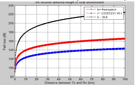
The receiver antenna heights are same as used earlier. Here we considered 20 m for transmitter antenna height. The ECC-33 model is not applicable in rural area and the COST 231 W-I model has no specific parameters for rural area, we consider LOS equation provided by this model. The numerical results for different models in rural area for different receiver antenna heights are shown in Figure

Figure :Path loss in rural area environment at 3 m receiver antenna height.

V. ANALYSISOFSIMULATIONRESULTS

Analysis of simulation results in urban area : The

accumulated results for urban environment are shown in Figure 6.1. Note that Ericsson model showed the lowest prediction (142 dB to 138 dB) in urban environment. It also showed the lowest fluctuations compare to other models when we changed the receiver antenna heights. In that case, the ECC-33 model showed the heights path loss (167 dB) and also showed huge fluctuations due to change of receiver antenna height. In this model, path loss is decreased when increased the receiver antenna height. Increase the receiver antenna heights will provide the

more probability to find the better quality signal from the transmitter. COST 231 W-I model showed the biggest path loss at 10 m receiver antenna height.

Analysis of simulation results in suburban area: The

accumulated results for suburban environment are shown in Figure 6.2. In following chart, it showed that the SUI model predict the lowest path loss (121 dB to 115 dB) in this terrain with little bit flections at changes of receiver antenna heights. Ericsson model showed the heights path loss (157 dB and 156 dB) prediction especially at 6 m and 10 m receiver antenna height. The COST-Hata model showed the moderate result with remarkable fluctuations of path loss with-respect-to antenna heights changes. The ECC-33 model showed the same path loss as like as urban environment because of same parameters are used in the simulation.

Analysis of simulation results in rural area:

The accumulated results for rural environment are shown in Figure 6.3. In this environment COST 231 Hata model showed the lowest path loss (129 dB) prediction especially in 10 m receiver antenna height and also showed significant fluctuations due to change the receiver antenna heights. COST 231 W-I model showed the flat results in all changes of receiver antenna heights. There are no specific parameters for rural area. In our simulation, we considered LOS equation for this environment (the reason is we can expect line of sight signal if the area is flat enough with less vegetations). Ericsson model showed the heights path loss (173 dB to 168 dB) which is remarkable, may be the reason is the value of parameters a0 and a1 are extracted by the LS methods

VI. CONCLUSION

Page | 28

that case, we may consider LOS calculation.

Alternatively, if there is less probability to get LOS signal, in that situation, we can see COST-Hata model showed the less path loss compare to SUI model and Ericsson model especially in 10 m receiver antenna height. But considering all receiver antenna heights SUI model showed less path loss whereas COST-Hata showed higher path loss.

If we consider the worst case scenario for deploying a coverage area, we can serve the maximum coverage by using more transmission power, but it will increase the probability of interference with the adjacent area with the same frequency blocks. On the other hand, if we consider less path loss model for deploying a cellular region, it may be inadequate to serve the whole coverage area. Some users may be out of signal in the operating cell especially during mobile condition. So, we have to trade-off between transmission power and adjacent frequency blocks interference while choosing a path loss model for initial deployment.

In future, our simulated results can be tested and verified in practical field. We may also derive a suitable path loss model for all terrain. Future study can be made for finding more suitable parameters for Ericsson and COST 231 W-I models in rural area.

REFERENCES

[1] V.S. Abhayawardhana, I.J. Wassel, D. Crosby, M.P. Sellers, M.G. Brown, “Comparison of empirical propagation path loss models for fixed wireless

access systems,” 61th IEEE Technology

Conference, Stockholm, pp. 73-77, 2005.

[2] Josip Milanovic, Rimac-Drlje S, Bejuk K,

“Comparison of propagation model accuracy for WiMAX on 3.5GHz,” 14th IEEE International conference on electronic circuits and systems, Morocco, pp. 111-114. 2007.

[3] Joseph Wout, Martens Luc, “Performance

evaluation of broadband fixed wireless system based on IEEE 802.16,” IEEE wireless communications and networking Conference, Las Vegas, NV, v2, pp.978-983, April 2006.

[4] V. Erceg, K.V. S. Hari, M.S. Smith, D.S. Baum, K.P. Sheikh, C. Tappenden, J.M. Costa, C. Bushue, A. Sarajedini, R. Schwartz, D. Branlund, T. Kaitz, D. Trinkwon, "Channel Models for Fixed Wireless Applications," IEEE 802.16 Broadband Wireless Access Working Group, 2001.

[5]

http://www.wimax360.com/photo/global-wimax-deployments-by [Accessed: June 28 2009]

[6] M. Hata, “Empirical formula for propagation loss in land mobile radio services,” IEEE Transactions on Vehicular Technology, vol. VT-29, pp. 317-325, September 1981.

[7] Rony Kowalski, “The Benefits of Dynamic

Adaptive Modulation for High Capacity Wireless Backhaul Solutions”, Ceragon Networks, [Online]. Available:http://www.ceragon.com/files/The%20Be nefits%20of%20Dynamic%20Adaptive%20Modulat ion.pdf [Accessed: April 18, 2009].