Vol. 10, No. 8, 2019
Empirical Study of Segment Particle Swarm
Optimization and Particle Swarm Optimization
Algorithms
Mohammed Adam Kunna Azrag1, Tuty Asmawaty Abdul Kadir2 Faculty of Computer Science & Software Engineering
Universiti Malaysia Pahang, Kuantan, Malaysia
Abstract—In this paper, the performance of segment particle swarm optimization (Se-PSO) algorithm was compared with that of original particle swarm optimization (PSO) algorithm. Four different benchmark functions of Sphere, Rosenbrock, Rastrigin, and Griewank with asymmetric initial range settings (upper and lower boundaries values) were selected as the test functions. The experimental results showed that, the Se-PSO algorithm achieved better results in terms of faster convergences in all the testing cases compared to the original PSO algorithm. However, the experimental results further showed the Se-PSO as a promising optimization algorithm method in some other different fields.
Keywords—Se-PSO; PSO; sphere; Rosenbrock; Rastrigin; Griewank
I. INTRODUCTION
Within the last two decades, optimization algorithms with mathematical programing have proved to be effective in solving large complex optimization problems. Recently, swarm intelligence techniques have gained popularity because of their capacity to locate partially optimal solutions for combinatorial optimization problems [1, 2]. These techniques have been applied in various areas, such as economics, engineering, bioinformatics, and industry. These problems are better solved using swarm intelligence techniques because they are usually very hard to solve accurately due to the lack of any precise algorithm to solve them [1, 2]. The swarm intelligence algorithms mainly depend on updating the population of individuals by applying some operators according to the fitness information obtained from the environment. With these updates, the individuals in a population are expected to move towards an optimum solution.
The Particle Swarm optimization (PSO) is one of the popular swarm algorithms which were formulated in 1995 by Dr. Kennedy and Eberhart. The PSO algorithm simulates the flocking behavior of birds and the schooling of fishes in order to achieve complex solutions [3-5]. The PSO algorithm is easy to execute and requires few parameters to be adjusted; it is computationally proficient and has a faster speed and premature convergence towards optima compared to Genetic Algorithm (GA) and Simulating Annealing (SA) algorithm [4]. It also has a flexible and well-balanced mechanism of improving its exploration capabilities [6]. The scenario of PSO is started by initializing a population of random solutions. Each potential solution is assigned with a randomized velocity, and the potential solutions are called particles. Each particle has its
own position, velocity, and fitness used to decide its best or bad positions in the solution space. The particle search depends on the personal best position (pbest) and the global best position (gbest) of each particle [7]. Moreover, the ability of PSO to find an optimum solution in reasonable time creates the need for its continuous improvement [8]. However, a segmentation of the PSO is implemented in this study to improve its convergence and accuracy using 4 optimization functions problem.
The rest of this paper is organized thus: the second section discusses the methodology of the PSO and the implemented Se-PSO algorithms. The third section explains the experimental setup and discussion of the results. The fourth section provides the conclusions drawn from the study.
II. METHODOLOGY
This paper presents the implementation method of Se-PSO with the comparison of PSO algorithms. The description of Se-PSO and Se-PSO is given in Pseudo code in Algo (1 and 2). Se-PSO algorithm is developed according to conventional Se-PSO algorithm. Thus, it has to go through the same procedures initialization of the bird’s step, number of birds, iteration, the problem dimension, and the position/velocity updating evaluation processes. However, the segmentation of the problem is added to PSO algorithm in order to reduce the time with a few iterations. The segmentation technique is always providing a fast convergence that able to achieve the best initial local position.
A. PSO Algorithm
The PSO algorithm is simulating the behavior of birds flocking and fish schooling in order to solve optimization problem in D-dimensional search space. This algorithm was proposed in 1995 [9]. The initialization of PSO is start by a group of random particles (solutions) and then searches for the optimum solution by updating generations. Each particle is flown through the solution problem space, having its position based on the information from its own personal best position and the best particle of the swarm. The performance of each particle and how close from the global optimum is calculated using a fitness function of the optimization problem. Each particle flies through the D-dimensional solution space and maintains the current position of particle , the personal best position of the particle , and the current velocity of particle . The particle keeps track of its coordinates in the
solution space which are associated with best solution (fitness) it has achieved so far which stored at each iteration. This value is called pbest (personal best position). Another value of the (best) called gbest (global best position) tracked by the global version of the particle swarm optimizer is the overall best value, and its location obtained so far by any particle in the population. During the particle swarm optimization searching calculation for solution, at each time step, changing the velocity (accelerating) each particle toward its pbest and gbest. Were this calculation mathematically described by this equation:
( ) ( )
Where is the velocity of particle it iteration , is the position of particle at iteration , = ( , , …,
) is the personal best position of each particle till the
particle number and =( , , …, ) is the global best position of the entire particle till the particle number ; is an inertia weight parameter, are acceleration coefficients, are random number between 0 and 1, and is the dimension in the solution space. The PSO algorithm procedure can be summarized as shown below in Algo 1. Algo 1 1. Start 2. Initialize the , , , ; 3. Initialize the , , , ; 4. Calculate the 5. If 6. For each ; a. Iter =1, ;
b. Updating the velocity towards fitness: c. ( )
( );
d. Update the position towards fitness: e. ;
7. If ;
a. Print of each particles;
8. If return step 2 till the iteration found highly solution or finished.
9. End
B. Se-PSO Algorithm
The Segment Particle Swarm algorithm idea is to divide the PSO particles to searching groups that can be considered as segments [10]. The segmentation means to separate the problem into parts or segments which reach the solution easily. In addition, the idea of Segmentation PSO algorithm is to divide the initial values into segments to help PSO particles during the search for the optimal values finding a local best position that may the global best position is around it. The segmentation can be divided into more than two groups based on the dimension.
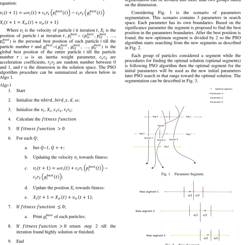
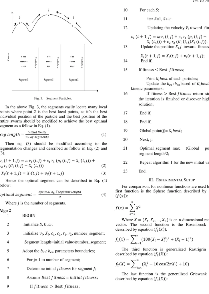
Considering Fig. 1 is the scenario of parameters segmentation. This scenario contains 3 parameters in search space. Each parameter has its own boundaries. Based on the significance parameter the segment is proposed to find the best position in the parameters boundaries. After the best position is found, the new optimum segment is divided by 2 so the PSO algorithm starts searching from the new segments as described in Fig. 2.
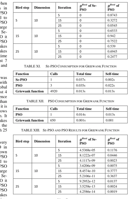
Each group of particles considered a segment while the procedures for finding the optimal solution (optimal segments) is following PSO algorithm then the optimal segment for the initial parameters will be used as the new initial parameters later PSO search in that range toward the optimal solution. The segmentation can be described in Fig. 3.
Search 1 Search 2 Search 3 Search 4 Seg 1 Seg 2 Seg 1 Seg 1 Seg 2 Parameter 1 Parameter 2 Parameter 3 Optimal segment
Fig. 1. Parameter Segment.
e/2 e/2 e/2 e/2 e/2 e/2 New segment 1 New segment 2 New segment 3
Vol. 10, No. 8, 2019
Segment 1 Segment 2 Segment 3
* *** ******* **** * ** ***** *** * ** ***** **** 1 2 3 P a rt ic le s P a rt ic le s P a rt ic le s Fi t n e s s * * *
Fig. 3. Segment Particles.
In the above Fig. 3, the segments easily locate many local points where point 2 is the best local points, as it’s the best individual position of the particle and the best position of the entire swarm should be modified to achieve the best optimal segment as a fellow in Eq. (1).
(1)
Then eq. (3) should be modified according to the segmentation changes and described as follow in Eq. (2) and (3).
(2) (3) Hence the optimal segment can be described in Eq. (4) below:
(4) Where is the number of segments.
Algo 2
1 BEGIN
2 Initialize ;
3 initialize , , , , , , number_segment; 4 Segment length=initial value/number_segment; 5 Adopt the parameters boundaries;
6 For j= 1 to number of segment; 7 Determine initial for segment ; 8 Assume = ; 9 If ;
10 For each ;
11 iter =1, ++;
12 Updating the velocity toward fitness:
;
13 Update the position toward fitness:
;
14 End if,
15 If fitness ;
Print of each particles;
Update the based of of each
kinetic parameters;
16 If fitness return step 2 till the iteration is finished or discover high-quality solution;
17 End if,
18 End if,
19 Global point(j)= ;
20 Next, j;
21 Optimal_segment=max (Global point) ±
segment length/2;
22 Repeat algorithm 1 for the new initial values;
23 End.
III. EXPERIMENTAL SETUP
For comparison, for nonlinear functions are used here. The first function is the Sphere function described by equation ( ):
∑
Where is an n-dimensional real-valued vector. The second function is the Rosenbrock function described by equation ( ):
∑
The third function is generalized Rastrigrin function described by equation ( ):
∑
The last function is the generalized Griewank function described by equation ( ):
∑
∏ ( √ )
TABLE I. LOWER AND UPPER BOUNDARIES
Function Lower and upper values
[-5, 5] [-5, 10] [-5.12, 5.12] [-600, 600]
Following the suggestion in [11] and for the purpose of comparison, the lower and upper values are selected to be as the original values. Table I lists the initialization of the upper and lower values of the four functions.
As in the above Table I, for each function, the maximum number of iteration is set to 50, 100, 150 in the both algorithms. The number of birds is set to 20, 40, 60, and 80. In order to compare the both algorithms inertia weight is adapted to 0.9. The learning factors . The dimension is 10 for
both. Each algorithm was tested 10 times to get the Mean global best position.
IV. RESULTS AND DISCUSSION
In Sphere function, the global best position of Se-PSO showed a very improved result in short time when compared to PSO. Moreover, as shown in Tables II and III the convergence speed of the Se-PSO towards the optimum values was faster when compared to PSO. It’s however, noticeable that the convergence of Se-PSO was quick in the all function but slowed down searching large space for the global best position before to be decided by Se-PSO algorithm as it approaches the optimal. The Se-PSO it took 0.213s to reach the best global position but the PSO reached the global best position in 0.033s. Where, Se-PSO takes 0.004s to decide the global best position while PSO takes 0.013s are depicted in Tables II and III in the self –time column. Moreover, Se-PSO searching large space almost 7 times of PSO as it described in the Calls column (4920 and 650) respectively.
Looking at Table IV where Sphere function was tested using Se-PSO and PSO on a 10-dimensional space with 5, 15, and 25 bird-step and 5, 15, and 25 iterations, the global best position of Se-PSO has very good result that is almost 4 times as good as the result of PSO. Moreover, the convergence speed of Se-PSO toward the optimum values are faster than those of PSO as showed in Tables II and III. Moreover, it is easy to observe that Se-PSO convergences quickly but slows its convergence speed down when reaching the optimum. It takes 0.004s to get the best global position while PSO takes 0.013s as can be seen clearly in Tables II and III. Finally, the total performance speed of the both algorithm is 0.213s with 25 iterations for Se-PSO and 0.033s only for PSO.
In Rastrigin function, the global best position of Se-PSO showed a very improved result in short time when compared to PSO in Table VII. Moreover, as shown in Tables V and VI the convergence speed of the Se-PSO towards the optimum values was faster when compared to PSO. It’s however, noticeable
that the convergence of Se-PSO was quick in the all function but slowed down searching large space for the global best position before to be decided by Se-PSO algorithm as it approaches the optimal. The Se-PSO it took 0.363s to reach the best global position but the PSO reached the global best position in 0.048s. Where, Se-PSO takes 0.001s to decide the global best position while PSO takes 0.013s are depicted in Tables V and VI in the self –time column. Moreover, Se-PSO searching large space almost 7 times of PSO as it described in the Calls column (4920 and 650), respectively.
TABLE II. SE-PSOCONSUMPTION FOR SPHERE FUNCTION
Function Calls Total time Self-time
Se-PSO 1 0.213s 0.004s
PSO 3 0.209s 0.030s
Sphere 4920 0.179s 0.179s
TABLE III. PSOCONSUMPTION FOR SPHERE FUNCTION
Function Calls Total time Self-time
PSO 1 0.033s 0.013s
Sphere 650 0.020s 0.020s
TABLE IV. SE-PSO AND PSORESULTS FOR SPHERE FUNCTION
Bird step Dimension Iteration
of Se-PSO of PSO 5 10 5 1.01335e-5 0.0701 15 2.12225e-06 0.0517 25 4.25101e-7 0.0074 15 10 5 3.25661e-07 0.0158 15 4.25861e-08 0.0132 25 1.05843e-08 0.0013 25 10 5 1.00035e-08 0.0001 15 2.03589e-09 0.0011 25 1.23565e-0.9 0.00002 TABLE V. SE-PSOCONSUMPTION FOR RASTRIGIN FUNCTION
Function Calls Total time Self-time
Se-PSO 1 0.363s 0.001s
PSO 3 0.362s 0.028s
Rastrigin function 4920 0.334s 0.334s
TABLE VI. PSOCONSUMPTION FOR RASTRIGIN FUNCTION
Function Calls Total time Self-time
PSO 1 0.048s 0.013s
Rastrigin Function 650 0.035s 0.035s
TABLE VII. SE-PSO AND PSORESULTS FOR RASTRIGIN FUNCTION
Bird step Dimension Iteration
of Se-PSO of PSO 5 10 5 1.1237e-05 1.0835 15 8.3919e-06 0.2655 25 3.5864e-06 0.9891 15 10 5 1.6515e-06 0.0028 15 2.2586e-07 0.0359 25 4.2056e-07 0.0026 25 10 5 3.0125e-08 0.0085 15 2.0123e-08 0.0064 25 1.0213e-09 0.003
Vol. 10, No. 8, 2019
In the Rosenbrock function, the global best position of Se-PSO showed a very improved result in short time when compared to PSO in Table X. Moreover, as shown in Tables VIII and IX, the convergence speed of the Se-PSO towards the optimum values was faster when compared to PSO. It’s however, noticeable that the convergence of Se-PSO was quick in the all function but slowed down searching large space for the global best position before to be decided by Se-PSO algorithm as it approaches the optimal. The Se-Se-PSO it took 0.158s to reach the best global position but the PSO reached the global best position in 0.03s. Where, Se-PSO takes 0.004s to decide the global best position while PSO takes 0.013s are depicted in Tables VIII and IX in the self –time column. Moreover, Se-PSO searching large space almost 7 times of PSO as it described in the Calls column (4920 and 650) respectively.
Looking at Table X above, where Rosenbrock function was tested using Se-PSO and PSO on a 10-dimensional space with 5, 15, and 25 bird-step and 5, 15, and 25 iterations, the global best position of Se-PSO has very good result that is almost 4 times as good as the result of PSO. Moreover, the convergence speed of Se-PSO toward the optimum values are faster than those of PSO as showed in Tables VIII and IX. Moreover, it is easy to observe that Se-PSO convergences quickly but slows its convergence speed down when reaching the optimum. It takes 0.004s to get the best global position while PSO takes 0.013s as can be seen clearly Tables VIII and IX. Finally, the total performance speed of the both algorithm is 0.158s with 25 iterations for Se-PSO and 0.030s only for PSO.
The global best position of Se-PSO showed a very improved result in short time when compared to PSO in Griewank function depicted in Table XIII. Moreover, as shown in Tables XI and XII the convergence speed of the Se-PSO towards the optimum values was faster when compared to PSO. It’s however, noticeable that the convergence of Se-PSO was quick in the all function but slowed down searching large space for the global best position before to be decided by Se-PSO algorithm as it approaches the optimal. The Se-Se-PSO it took 0.037s to reach the best global position but the PSO reached the global best position in 0.014s. Where, Se-PSO takes 0.002s to decide the global best position while PSO takes 0.013s are depicted in Tables XI and XII in the self –time column. Moreover, Se-PSO searching large space almost 7 times of PSO as it described in the Calls column (4920 and 650), respectively.
TABLE VIII. SE-PSOCONSUMPTION FOR ROSENBROCK FUNCTION
Function Calls Total time Self-time
Se-PSO 1 0.158s 0.004s
PSO 3 0.154s 0.026s
Rosenbrock function 4920 0.128s 0.128s
TABLE IX. PSOCONSUMPTION FOR ROSENBROCK FUNCTION
Function Calls Total time Self-time
PSO 1 0.030s 0.013s
Rosenbrock function 650 0.016s 0.016
TABLE X. SE-PSO AND PSORESULTS FOR ROSENBROCK FUNCTION
Bird step Dimension Iteration
of Se-PSO of PSO 5 10 5 0 0.8743 15 0 0.3272 25 0 0.0545 15 10 5 0 0.6533 15 0 0.942 25 0 0.7522 25 10 5 0 0.539 15 0 0.6945 25 0 0.2477 TABLE XI. SE-PSOCONSUMPTION FOR GRIEWANK FUNCTION
Function Calls Total time Self-time
Se-PSO 1 0.037s 0.002s
PSO 3 0.035s 0.022s
Griewank function 4920 0.013s 0.013s
TABLE XII. PSOCONSUMPTION FOR GRIEWANK FUNCTION
Function Calls Total time Self-time
PSO 1 0.014s 0.013s
Griewank function 650 0.001s 0.001
TABLE XIII. SE-PSO AND PSORESULTS FOR GRIEWANK FUNCTION
Bird step Dimension Iteration
of Se-PSO of PSO 5 10 5 4.5368e-05 0.1176 15 8.1222e-07 0.0446 25 4.1117e-09 0.0023 15 10 5 3.6206e-09 0.0075 15 8.4574e-10 0.3777 25 5.2106e-11 0.3637 25 10 5 9.2952e-12 0.0137 15 3.5258e-13 0.0024 25 4.2586e-14 0.0019 V. CONCLUSION
The Se-PSO algorithm was introduced in this study through the incorporation of a segmentation solution during the searching process by the particles into the original version of the PSO. After this, the best segment position of Se-PSO algorithm was projected as the new search dimension to find the optimum values. To investigate the proposed method, four functions were employed. The results of the experiments showed that the Se-PSO exhibited fast convergence when compared with the ABO. Although it was observed that the Se-PSO algorithm worked efficiently, the need for further experiments on more complex multimodal, separable and non-separable functions cannot be ruled out in order to further validate the search capacity of the Se-PSO. Moreover, there is a need to apply the proposed Se-PSO to other optimization search landscapes such as urban transportation problems, job scheduling, dynamic modeling, and vehicle routing.
ACKNOWLEDGMENT
The authors gratefully acknowledge the financial support from the Universiti Malaysia Pahang and FSKKP under PGRS190312 and FRGS under Grant RDU 160101. The authors would like to thank Dr. Tuty Asmawaty Abdul Kadir, who supervised this work.
REFERENCES
[1] Soliman, Soliman Abdel-Hady, and Abdel-Aal Hassan Mantawy. Modern optimization techniques with applications in electric power systems. Springer Science & Business Media, 2011.
[2] Venter, Gerhard. "Review of optimization techniques." Encyclopedia of aerospace engineering (2010).
[3] Kennedy, James. "Particle swarm optimization." Encyclopedia of machine learning. Springer, Boston, MA, 2011. 760-766.
[4] Eberhart, Russell C., and Yuhui Shi. "Comparison between genetic algorithms and particle swarm optimization." International conference on evolutionary programming. Springer, Berlin, Heidelberg, 1998. [5] Khare, Anula, and Saroj Rangnekar. "A review of particle swarm
optimization and its applications in solar photovoltaic system." Applied Soft Computing 13.5 (2013): 2997-3006.
[6] Banks, Alec, Jonathan Vincent, and Chukwudi Anyakoha. "A review of particle swarm optimization. Part I: background and development." Natural Computing 6.4 (2007): 467-484.
[7] Banks, Alec, Jonathan Vincent, and Chukwudi Anyakoha. "A review of particle swarm optimization. Part II: hybridisation, combinatorial, multicriteria and constrained optimization, and indicative applications." Natural Computing 7.1 (2008): 109-124.
[8] Shi, Yuhui. "Particle swarm optimization: developments, applications and resources." evolutionary computation, 2001. Proceedings of the 2001 Congress on. Vol. 1. IEEE, 2001.
[9] Poli, Riccardo, James Kennedy, and Tim Blackwell. "Particle swarm optimization." Swarm intelligence 1.1 (2007): 33-57.
[10] Jaber, Aqeel S., Abu Zaharin Ahmad, and Ahmed N. Abdalla. "A new parameters identification of single area power system based LFC using Segmentation Particle Swarm Optimization (SePSO) algorithm." Power and Energy Engineering Conference (APPEEC), 2013 IEEE PES Asia-Pacific. IEEE, 2013.
[11] Shi, Yuhui, and Russell C. Eberhart. "Empirical study of particle swarm optimization." Evolutionary computation, 1999. CEC 99. Proceedings of the 1999 congress on. Vol. 3. IEEE, 1999.