Dissertation
submitted to the
Combined Faculties for the Natural Sciences and for Mathematics
of the Ruperto-Carola University of Heidelberg, Germany
for the degree of
Doctor of Natural Sciences
put forward by
Dipl.-Phys. Matthias Wieler
born in Mannheim, Germany
Multiple Instance Learning
with Random Forests
and Applications in Industrial Optical Inspection
Referees: Prof. Dr. Fred A. Hamprecht
Prof. Dr. Luca Amendola
Hiermit erkl¨are ich, da ich die vorliegende Dissertation selbst verfasst und mich dabei keiner anderen als der von mir ausdr¨ucklich bezeichneten Quellen and Hilfen bedient habe. Des Weiteren erkl¨are ich, dass ich an keiner anderen Stelle ein Pr¨ufungsverfahren beantragt oder die Dissertation in dieser oder einer anderen Form bereits anderweitig als Pr¨ufungsarbeit verwendet oder einer anderen Fakult¨at als Dissertation vorgelegt habe.
Heidelberg,
Zusammenfassung
F¨ur die automatische Defekterkennung in der industriellen optischen Inspektion werden Al-gorithmen ben¨otigt, die aus Daten lernen. Eine besondere Herausforderung sind Daten mit unvollst¨andigen Labels. Eine der Methoden, die das Feld des maschinellen Lernens her-vorgebrachte hat um mit unvollst¨andigen Labels umzugehen, ist das sog. Multiple Instance Learning. Ein Merkmal dieses Ansatzes ist, dass dabei die Datenpunkte (Instanzen) zu sog. Bags zusammenfasst werden.
Wir schlagen eine neue Methode zur Berechnung der Bag-Wahrscheinlichkeiten aus den Instanz-Wahrscheinlichkeiten vor, die den Vorteil hat, dass die Ergebnisse nicht von der Gr¨oße der Bags abh¨angig sind. Weiterhin schlagen wir eine Erweiterung des Multiple In-stance Modells vor, das es dem Benutzer erlaubt, die Anzahl der als positiv klassifizierten Instanzen zu steuern.
Wir implementieren diese Methoden mit einem Algorithmus, der auf dem wohlbekan-nten Random Forest-Klassifikator aufbaut. Der Algorithmus zeigt auf einem bekanwohlbekan-nten Benchmark-Datensatz eine konkurrenzf¨ahige Klassifikationsleistung. Wir wenden diesen Al-gorithmus auf Bilddaten an, die die Besonderheiten der industriellen optischen Inspektion widerspiegeln, und zeigen, dass der Algorithmus in diesem Szenario den normalen Random Forest ¨ubertrifft.
Abstract
Automatic defect detection in industrial optical inspection requires algorithms that can learn from data. A special challenge is data with incomplete labels. One of the methods that the field of machine learning has brought forth to deal with incomplete labels is multiple instance learning. One trait of this setting is that it groups datapoints (instances) into bags. We propose a novel method to predict bag probabilities from given instance probabilities that has the advantage that its results do not depend on bag size. Also, we propose an extension of the multiple instance model that allows the user to steer the number of instances that are classified as positive.
We implement these methods with an algorithm based on the well-known random forest classifier. Results on a standard benchmark dataset show competitive performance. Fur-thermore, we apply this algorithm to image data that reflects the challenges of industrial optical inspection, and we show that in this setting it improves over the standard random forest.
Acknowledgments
I am indebted to my supervisor Prof. Fred A. Hamprecht. Without him I would probably not have discovered the exciting field of machine learning. He did not spare any effort to give me scientific advice. I am grateful for his unlimited support both in good times and in bad times.
I would also like to thank all my colleagues in the multidimensional image processing group, who gave me valuable scientific input, in particular Ullrich K¨othe, Nikos Gianniotis, Bj¨orn Andres, Michael Hanselmann, Melih Kandemir, Frederik Kaster, Christoph Sommer, Bernhard Kausler, Marc Kirchner, and Xinghua Lou.
This work has been supported by Robert Bosch GmbH. I would like to cordially thank the persons in charge for making this possible. Special thanks go to Walter Happold who gave me all support I could wish for.
I would like to thank my advisers at Bosch, Christian Perwass and Ralf Zink, for many valuable discussions. I have profited from their advice.
Working on this thesis would have been less joyful without my colleagues at Bosch. In particular, I wish to thank Jens R¨oder for the numerous scientific discussions and personal conversations we have had. Cordial thanks go to my fellow doctorate students, namely Andreas Walstra, Patrick Sauer, Joachim B¨orger, Andreas Gr¨utzmann, Thomas Geiler, Marc J¨ager, Linus G¨orlitz, and Stefan Trittler.
Also I would like to thank Prof. Luca Amendola, Prof. R¨udiger Klingeler, and Prof. Bernd J¨ahne for serving on my committee.
Contents
Acknowledgments v
Contents vi
1 Introduction 1
1.1 Industrial optical inspection . . . 1
1.2 Image processing . . . 2
1.3 Machine learning . . . 3
1.4 Weak labels and multiple instance learning . . . 4
1.5 DAGM datasets . . . 4
2 Bayesian Learning Theory 7 2.1 The general setting . . . 7
2.2 Inference . . . 9
2.2.1 Maximum posterior and maximum likelihood . . . 10
2.2.2 Bayesian averaging . . . 11
2.2.3 Bagging . . . 11
2.3 Generative and discriminative models . . . 13
2.4 Semi-supervised learning . . . 16
2.4.1 Self-training . . . 17
2.5 Learning from weak labels . . . 19
2.5.1 Noisy labels . . . 19
2.5.2 Bag labels . . . 20
2.5.3 Inference in bag models . . . 21
3 Multiple Instance Learning 23 3.1 The multiple instance model . . . 23
3.1.1 Model definition . . . 23
3.1.2 Model training . . . 25
3.1.3 Relation to semi-supervised learning . . . 26
3.2 Interpretations and variants of the multiple instance model . . . 27
3.2.1 Standard MI (sMI): Estimate latent instance classes . . . 27
3.2.2 Discard non-positive instances (dMI) . . . 27
3.2.3 Sesqui-class learning (SCL) . . . 30
3.3 Applications . . . 35
3.3.1 Drug activity prediction . . . 35
3.3.2 Image classification . . . 36
3.3.3 Others . . . 36
3.4 Algorithms . . . 37
3.4.1 Axes-parallel rectangles (APR) . . . 37
3.4.2 Diverse density (DD) . . . 38
3.4.3 Diverse density with expectation maximization (EM-DD) . . . 39
3.4.4 Multiple instance SVMs . . . 40
3.4.5 Multiple instance learning based on decision trees . . . 41
3.4.6 Others . . . 42
4 Improving Multiple Instance Classification 43 4.1 Bag size independent multiple instance classification . . . 43
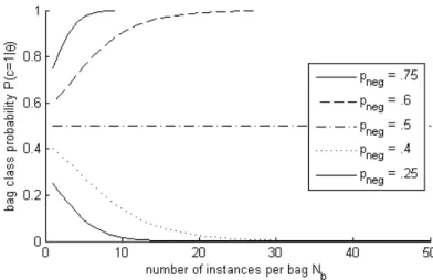
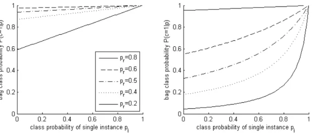
4.1.1 Bag size dependent bias . . . 44
4.1.2 Generative, discriminative, and general bag models . . . 45
4.1.3 The generative multiple instance model . . . 47
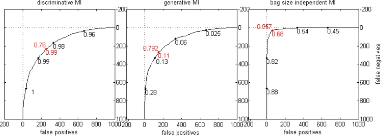
4.1.4 Bag size independent MI model . . . 50
4.1.5 Assessment on synthetic data . . . 52
4.2 Multiple instance classification with ensemble classifiers . . . 54
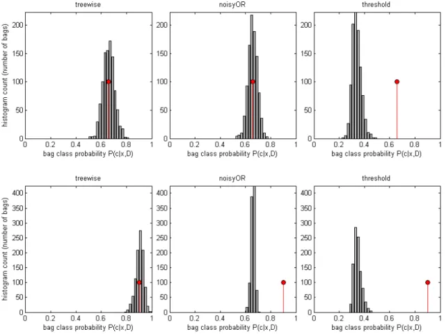
4.2.1 Ensemble average at bag level . . . 54
4.2.2 Ensemble average at instance level . . . 55
4.2.3 Overview of bag classification methods . . . 57
4.2.4 Experimental results . . . 58
5 Alternative Bag Models for Multiple Instance Applications 63 5.1 Bernoulli model . . . 63
5.1.1 Model definition . . . 63
5.1.2 Model properties . . . 64
5.1.3 Combination with MI model . . . 66
5.1.4 Notes on the Bernoulli model . . . 70
5.2 Power model . . . 73
5.2.1 Model definition . . . 73
5.2.2 Implementation . . . 75
6 Self-Training Multiple Instance Random Forest (SMIRF) 77 6.1 Random forests . . . 77
6.2 Self-training random forest for standard multiple instance learning . . . 80
6.2.1 Self-training the multiple instance model . . . 80
6.2.2 Sampling approach and out-of-bag estimate . . . 81
6.2.3 Algorithm details and behavior . . . 83
6.3 Results on MUSK datasets . . . 87
6.3.2 Bag-size-independent classification . . . 89
6.4 Results on DAGM data . . . 94
6.4.1 Bag classification via threshold method . . . 94
6.4.2 SMIRF with power model . . . 96
7 Conclusion 100
Chapter 1
Introduction
The starting point of this work has been the application of industrial optical inspection. Optical inspection is a widespread method to ensure the quality of components or devices directly after production. As in many areas, there is a need for automation to reduce cost and increase reliability. However, one drawback of automated optical inspection is the loss of flexibility compared to human visual inspection.
Recent advances in the field of machine learning make algorithms available that can learn from examples. These methods promise improved flexibility because it is easier to retrain a machine learning algorithm than to adapt an image processing algorithm to new requirements or boundary conditions.
The subject of this thesis is multiple instance learning, which is a machine learning setting that corresponds to the special requirements of industrial optical inspection. But before going into the details of multiple instance learning, we give an introduction of industrial optical inspection and image processing and describe the role of machine learning in this setting. Also, we present a datasets that we have used to assess our multiple instance learning methods for the target application of industrial optical inspection.
1.1 Industrial optical inspection
Industrial optical inspection is a method of quality control. The production process of technical devices usually involves many steps and can be quite complex. Even when great care is taken, it is often not possible to completely rule out that an error occurs. To make sure that the final product is free of defects, it is usually necessary to perform several inspections and/or tests.
Optical inspection is a suitable method in many cases because it is fast and very versatile. Often, it can be used to detect several different kinds of defects with a single inspection. Optical inspection can either be performed by humans, or it can be an automated system. Human visual inspection Even in highly automated production lines human visual in-spection is still common. The reason is that the flexibility and versatility of human visual inspection is very hard to achieve with an automated system (Kleeven & Hyv¨arinen 1999). Humans have an extremely good image understanding and can detect a wide variety of possible defects with little or even no training or instructions.
Chapter 1 Introduction
The main disadvantage of human visual inspection (besides cost) is the subjectivity and varying quality of human assessment (Schoonard, Gould & Miller 1973). Different inspectors often have different opinions as to whether a given component is to be classified as intact or as defective. Even a single inspector’s assessment can be subject to fluctuation, caused by tiredness or other factors.
Automated optical inspection Automated optical inspection usually includes a handling device to position the components, special lighting, a camera with suitable optics and filters, and an image processing system. Handling and image acquisition can typically be performed within a few seconds or less, which allows for inspection of a component within the cycle time of serial production. Suitable lighting, optics, and filters are often essential to make the defects of interest clearly visible. A general rule is that the more effort is spent on image acquisition the less effort has to be spent later on image processing. For a more detailed introduction see (Demant, Streicher-Abel & Springhoff 2011) or (Beyerer, Le´on & Frese 2012).
1.2 Image processing
Image processing deals with the problem of finding meaningful descriptions of an image from the raw data (matrix of gray values). This task can be divided into three steps: preprocess-ing, feature extraction, and image analysis (J¨ahne 2012). Preprocessing includes operations on single pixels like color adjustment or interpolation. The goal of feature extraction is to calculate local features from a small neighborhood of pixels. These features describe basic elements of the image like edges, ridges, corners, etc. Image analysis, finally, tries to provide a good high-level description of the image based on local features.
In industrial optical inspection, the final goal is to classify an image as either “intact” or “defective”. Sometimes it is also required to specify which type of defect has occurred.
The third step of image analysis and classification can either by performed with classical image processing or with machine learning methods.
Classical image analysis Classical image analysis is state of the art in industrial optical inspection. It includes operations like image segmentation, morphological operations, quan-titative characterization of the segments, inverse filtering, and others. While most problems can be solved with this approach, the solutions are very application-specific. It is necessary to develop and optimize the algorithm specifically for each application and type of defect, which often involves careful tuning of many parameters, setting decision thresholds, etc.
In industrial optical inspection, the requirements and boundary conditions for image classification change regularly because of variations in the production process, changing customer demands, or because new types of defects arise. This requires regular adjustment of the image analysis algorithm which causes considerable effort. To reduce the cost of adaptation, a different approach based on machine learning is necessary.
Chapter 1 Introduction
series production
change of requirements and/or boundary conditions image acquisition feature extraction image classification
training data
human inspector
training of algorithm
intact defective
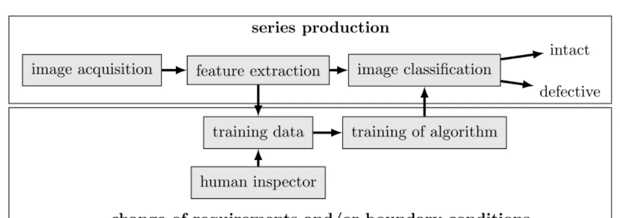
Figure 1.1: Overview of applying machine learning in industrial optical inspection.
1.3 Machine learning
Machine learning concerns the development of algorithms that can learn from examples. It has the potential to reduce the effort of customization and adaption of image processing systems significantly.
The setting of machine learning in industrial optical inspection is illustrated in Figure 1.1. It includes both the continually running series production (upper box), and the occasional adjustment to new requirements and boundary conditions (lower box). In series production, an important requirement on the inspection system is speed. Feature extraction and image classification must be executed within the fixed cycle time. The main concern of system adaptation (lower box) is to ensure the accuracy of image classification (i. e. the reliability of inspection) and to minimize the amount of human work.
The core subject of machine learning (and of this thesis) is algorithm training and image classification (rightmost text boxes). For the application in industrial optical inspection and to test the performance of the algorithms, we also have to consider feature extraction and training data.
Training data Training a machine learning algorithm requires a training dataset that con-sists of (i) example images of intact and defective components and (ii) a label for each image describing whether it is “intact” or “defective”. The example images can usually be acquired easily with the available image acquisition device, but the labels must be provided by a human inspector.
Note that labeled example images are needed both for machine learning and for classical image analysis. However, machine learning is more dependent on the amount and quality of the training data than classical image analysis. A human image processing expert can work with unstructured and incomplete data, and few example images are often sufficient. Machine learning, on the contrary, requires a complete dataset in a fixed format, and more
Chapter 1 Introduction
example images are needed to achieve good accuracy.
The increased effort of acquiring training data mitigates the benefit of automated training. On the other hand, it increases objectivity and quantifiability. In machine learning, the training data and accuracy estimates are documented as a matter of course, and the result can be reproduced and checked at any time. This is not necessarily the case in classical image analysis, where there is less emphasis on training data and statistical estimates of prediction accuracy.
1.4 Weak labels and multiple instance learning
To keep labeling effort within acceptable limits, it is not possible to label each defect exactly on the pixel-level. Instead, we have to use labels on either the image-level (image is labeled as a whole) or on the region-level (the image region containing the defect is specified). In both cases the regions labeled as “defective” contain (besides the defect) a considerable percentage of the “intact” image. In this sense the provided labels are “weak”.
The central topic of this thesis is to develop machine learning algorithms that can deal with this kind of weak labels. Although it is possible to use standard supervised machine learning methods with weak labels, the mislabeled datapoints (labeled “defective” although they are in fact “intact”) impair classification accuracy. We have found that the so-called “multiple instance” setting is a suitable model for this task. While this model has originally been proposed for a different application (see Chapter 3), it can also be used for weakly labeled images. However, one can improve over the multiple instance model by using additional information about the size of the defect (i. e. the number of truly “defective” pixels), which will be the topic of Chapter 5.
1.5 DAGM datasets
To assess our proposed machine learning methods for the target application of industrial optical inspection, we have created an artificially generated benchmark dataset. It has been designed to imitate real world problems of industrial optical inspection. The data has been published1 at the DAGM2 symposium.
The DAGM data consists of 10 different datasets, each consisting of 1000 images showing the background texture without defects, and 150 images showing the background texture with one defect. The images in a single dataset are very similar, but each dataset is generated by a different texture model and defect model. The images are 8-bit grayscale with size 512-by-512. Example images are shown in Figure 1.2.
The defects are labeled by ellipses covering the defects. These labels are not exact on a pixel-level, but are weak in the sense described above. Thus the DAGM datasets are well suited to test the multiple instance learning algorithms proposed in this thesis.
1
http://hci.iwr.uni-heidelberg.de/Staff/dagm2007/prizes.php3#industry
Chapter 1 Introduction
Image features used for DAGM datasets Before image classification we need to extract local image features. Based on the work of (Sauer 2008), we chose a two-step approach to feature calculation. The first step consists of a wavelet filter bank, the second step consists of statistics calculated over small image patches.
For the first step we chose the so-called a “steerable pyramid” proposed by (Simoncelli & Freeman 1995, Karasaridis & Simoncelli 1996). This is a wavelet filter bank that comprises a set of oriented bandpass filters, yielding a radial-axial decomposition of frequency domain. We chose a resolution of 4 different scales and 6 different orientations, which gives a total of 24 different feature images.
For the second step we used patches of size 32-by-32 pixels with an overlap of 16 pixels (giving a total of 32-by-32 patches per image). Over each patch we calculated the 5 following statistics: minimum, maximum, mean, variance, and kurtosis. Note that the steerable pyramid outputs images of different resolution depending on the scale used, so the statistics are calculated over a different number of pixels of the pyramid result.
In addition to the above 120 features we used the position of the patch in the image (x -and y-coordinates) as two additional features. These features are useful for classification if the defects are located mainly in one region of the image (Class 7) or if the appearance of the defects depend on the location (Class 4).
Chapter 2
Bayesian Learning Theory
This chapter gives an overview of statistical theory for machine learning from a Bayesian viewpoint. The goal is to provide the theoretical foundation needed in later chapters.
We focus on the topics of semi-supervised learning and bag models (of which the multiple instance model is a special case), generative vs. discriminative learning (which is a prerequi-site for the bag-size-independent MI model of Section 4.1), self-training, and bagging (which are needed for our proposed learning algorithm in Section 6). To obtain a coherent text, we found it necessary to also include some general topics.
The emphasis of this chapter is slightly more theoretical than standard expositions of machine learning. Of the well-known text books, our treatment is closest to (Bishop 2006).
2.1 The general setting
Machine learning is about the relation between an input x and an output y. For given inputs x one would like to predict the corresponding outputs y. The problem is that the relation itself is unknown. The only available information are examples of corresponding input-output pairs (xn, yn), thetraining data.
The inputxis usually continuous and high-dimensional, the outputyis most often binary (positive or negative), but sometimes also categorical (multiclass learning) or continuous (regression).
Formally, the relation betweenxand y can most generally be described by a probability distribution
Ptrue(x, y). (2.1)
Since this true distribution is unknown, one tries to model it with a set of candidate distri-butions, that are described by parametersθ
P(x, y|θ). (2.2)
A specific distribution (represented by its parameter vector θ) is called a concept or an
hypothesis, and the parameter space Θ defines a set of possible concepts or an hypothesis space. One usually assumes that there is one true parameter vector θtrue that correctly
Chapter 2 Bayesian Learning Theory
describes the underlying distribution
Ptrue(x, y) = P(x, y|θtrue). (2.3) xn yn θ xm ym N M
Figure 2.1: Markov net-work of supervised learn-ing. Left side: N training data points. Right side:
M test points. Shaded nodes represent observed variables, unshaded nodes must be inferred.
Since the true parameter vector is unknown, we have to consider a probability distribution over the parameters
P(θ). This parameter prior is often taken as uniform, but one can also define a non-uniform parameter prior that makes certain concepts more likely than others. So most generally, a probabilistic learning model is described by
P(x, y,θ) = P(x, y|θ)·P(θ). (2.4) This model can be represented by the Markov network shown in Figure 2.1. All datapoints are linked by the com-mon concept θ. The training data points are grouped on the left side, the test points on the right side. Indexnruns from 1 toN, indexm runs fromN+ 1 toN+M. The task is to infer the test outputsym from the test inputsxm and
the training dataD={xn, yn}via the latent parametersθ.
Besides this data-centered viewpoint, it is useful to consider the complete distribution of xand y, which is a superposition of the candidate distributions, weighted by the parameter distribution
P(x, y) =
Z
P(x, y|θ)P(θ) dθ. (2.5) This distribution can be seen as the intermediate result Note that we should require the prior (x, y)-distribution to be uniform
P(x, y) = U(x, y), (2.6)
otherwise the learning model (2.4) would be prejudiced. This requirement is met by standard learning techniques, but it is usually not stated explicitly.
After having observed the dataD, the prior (2.5) is replaced by the posterior
P(x, y| D) =
Z
P(x, y|θ)P(θ| D) dθ. (2.7)
Note that the posterior distribution (2.7) is not necessarily contained in the set of candidate distributions (2.2), so one could say that Bayesian inference “increases the flexibility” of prediction (Minka 2000).
Chapter 2 Bayesian Learning Theory
Train-test split and transduction Note that the symbolDin (2.7) stands forall data, i. e. both training data and test data
D = Dtrain∪ Dtest = {xn, yn} ∪ {xm}. (2.8)
In fact, the posterior parameter distribution depends in general not only on the training data but also on the test data.
P(θ| D) = 1 Z P| {z }(θ) prior Y n P(xn, yn|θ) | {z } training likelihood Y m P(xm|θ) | {z } test likelihood . (2.9) Z = P(D) = Z Y n P(xn, yn|θ) Y m P(xm|θ) dθ (2.10)
The test likelihood is usually neglected. In most cases this is does not cause a significant difference, because the information contained in the training data usually outweighs the information contained in the test data (i. e. the training likelihood has a sharper peak than the test likelihood).
xn yn θ θ xm ym N M
Figure 2.2: Markov networks of training stage (left side) and testing stage (right side). Note that during testing, θ does not actually have a fixed value (which would be the usu-ally meaning of a shaded node), but a fixed distribution. Nevertheless we find that the shaded node expresses the idea clearly enough.
The benefit of neglecting the test likelihood is that it simplifies inference by effectively splitting it in two subsequent steps: training and testing. During training one infers the posterior parame-ter distributionP(θ| Dtrain) by taking into account the training data, but neglecting the test data. During testing one holds the parameter distribu-tion constant and evaluates (2.11). This setting is shown in Figure 2.2.
The fact that the test data contain potentially useful information does not seem to be generally appreciated. In the context of semi-supervised learn-ing it is more obvious, because unlabeled trainlearn-ing points are actually the same as test points (x is observed, y is not). In this context, the idea of using the test data in addition to training data to improve prediction is known astransduction. We will discuss this in more detail in Section 2.4.
2.2 Inference
In this section we discuss the main inference step of evaluating (2.7). As is common, we incorporate the train-test split and consider only the training data. Then, (2.7) and (2.9)
Chapter 2 Bayesian Learning Theory are replaced by P(x, y| Dtrain) = Z P(x, y|θ)P(θ| Dtrain) dθ (2.11) P(θ| Dtrain) ∝ P(θ)L(θ) (2.12) L(θ) = Y n P(xn, yn|θ) (2.13)
The integration overθ is usually infeasible because the parameter space is high-dimensional (it must be to allow for enough flexibility of the candidate distributions).
There are several approaches to find reasonable approximations for (2.11). They all have in common that they approximate (2.11) by a weighted sum.
P(x, y| Dtrain) ≈ X
t
wtP(x, y|θt) (2.14)
The differences between these methods is in how they choose the support points{θt}, and
how they estimate the weights wt. Note that in generalwt6=P(θt| Dtrain).
Methods that learn multiple conceptsθtare often calledensemble methodsorcommittees.
They include Bayesian averaging, bagging, boosting, and others. But also point estimation methods like maximum posterior and maximum likelihood can be thought of as special cases of (2.14), with only one support point.
2.2.1 Maximum posterior and maximum likelihood
Both the maximum posterior and the maximum likelihood approach are point estimation methods, which means that they learn only one concept and have only one support point ˆθ with weight 1. In this case the approximation (2.14) simplifies to
P(x, y| Dtrain) ≈ P(x, y|ˆθ). (2.15) It is obvious that the best choice of ˆθ is the maximum of the parameter posterior
ˆ
θMAP = arg max
θ
P(θ| D). (2.16)
To put it into words, the procedure is that one first tries to find the concept ˆθ within the model that best explains the training data. Then this concept is used to predict the test class.
Another common choice of ˆθ is the maximum likelihood estimate ˆ
θML = arg max
θ
L(θ) (2.17)
Although maximum likelihood is not originally a Bayesian method, it is quite natural to view it as an approximation of Bayesian inference as described above. Note that if the
Chapter 2 Bayesian Learning Theory
parameter prior is uniform P(θ) = U(θ), the maximum posterior estimate (2.16) equals the maximum likelihood estimate (2.17). Often one does not have cogent prior information about the model parameters, so one chooses a more or less flat prior. In this case the maximum of the parameter posterior is dominated by the likelihood.
Note that both from a conceptual and a practical point of view there is big difference between the Bayesian approach (2.11) and the maximum posterior or maximum likelihood approach. The Bayesian approach puts the emphasis on integration, while the maximum posterior/likelihood puts the emphasis on optimization. This entails very different tools and techniques.
2.2.2 Bayesian averaging
The goal of Bayesian averaging is to approximate the full Bayesian integral (2.11). This can be done with the averaging approach (2.14) by setting
θt ∼ P(θ| Dtrain) (2.18)
wt = P(θt| Dtrain) (2.19)
The difficulty of this approach is the large computational cost. Especially, sampling from the posterior parameter distribution P(θ| Dtrain) is hard, because θ is high-dimensional, and P(θ| Dtrain) is usually complex and multimodal.
2.2.3 Bagging
“Bagging” is an abbreviation of “bootstrap aggregating”. It has been proposed by (Breiman 1996). The idea is to repeatedly draw bootstrap samples from the training data (sampling with replacement), and then train a classifier on each set of bootstrapped training data. The final classifier is the average (or majority vote) of all single classifiers.
Formally, a bagged classifier is described by Eq. (2.14) with concepts θt = arg max
θ
P(θ| Dt) (2.20)
whereDtis the t-th set of bootstrapped samples, and uniform weights
wt=
1
T. (2.21)
The idea behind bagging is that taking the average over different datasets reduces the mean squared error of the prediction. It can easily be shown (Breiman 1996) that
ED(y−yˆD)2 ≥ (y−ED(ˆyD))2, (2.22)
where ED denotes expectation over all possible datasets, y is the true class, and ˆyD is the
estimate from datasetD. Thus the average ED(ˆyD) improves over the point estimate ˆyD.
Chapter 2 Bayesian Learning Theory
The problem is that bootstrapped samplesDtare not drawn from the true data
distribu-tionP(x, y), but are resampled from the observed data. Technically speaking, they do not follow the same distribution as the training data, but are distributed according to a mix of delta distributions at the observed datapoints
Dt ∼ D/ (2.23) Dt ∼ 1 T X n δ(xn)δ(yn). (2.24)
For some special models one can modify the bootstrapping procedure so that the inferred quantitiesθtandytare in fact distributed according to their posteriorsP(θ| D), orP(y| D),
even though the original samples are not (2.23). This is called the “Bayesian bootstrap” (Rubin 1981). For a complex machine learning model, however, this is not possible.
As a consequence of (2.23) we expect that the mean squared error of the bagged estimate is larger than the mean squared error of the hypothetical average of estimators
(y−EDt(ˆyDt))
2 ≥ (y−E
D(ˆyD))2. (2.25)
It is very difficult to exactly assess the size of the difference between the two sides of this inequality. Bagging works if the bagged estimate’s error (left hand side of 2.25) is at least smaller than the point estimate’s error (left hand side of 2.22).
Stability of classifier A measure to asses the size of inequality in (2.22) is the “stability” or “variability” of the classifier. This is a rather vague concept of how much the parameter estimate θt changes with changing data Dt. A perfectly stable classifier would have the
same optimum for all data samples,
θs = θt ∀s, t, (2.26)
and equality would hold in (2.22).
While some instability is needed to improve over the base classifier (i. e. inequality of 2.25), it seems plausible that too much instability will probably hurt performance, because the ensemble members trained on the bootstrapped samples deviate too much from the optimum point estimate
θt 6= θˆMAP, (2.27)
and we expect very large inequality in 2.25.
Bootstrap sample size For a given classifier, bagging provides one parameter to control the stability or variability ofθt: the bootstrap sample size Nboot. For very largeNboot, the
Chapter 2 Bayesian Learning Theory
converges to its base (non-bagged) classifier:
Nboot→ ∞ =⇒ Dt→ D =⇒ θt→θˆMAP (2.28)
This situation corresponds to a perfectly stable classifier. Likewise, a small bootstrap sample size corresponds to an unstable classifier.
Bagging has been shown to give good performance in many empirical settings. The most well-known example of the success of bagging is the so-called “random forest” (Breiman 2001), which is a bagged version of fully grown decision trees. For the random forest a bootstrap sample size equal to the number of available training points is the standard choice that usually gives good results (Hastie, Tibshirani & Friedman 2009). Because of the good reputation of the random forest, it will be the basis for our proposed algorithms for multiple instance learning (see Chapter 6).
2.3 Generative and discriminative models
Basic idea Up to now we have considered the general case of modeling the joint distribution
Ptrue(x, y) with a single set of parameters θ. It is suggestive to split this joint distribution
into a marginal and a conditional, and model the marginal and the conditional separately. There are two obvious ways to perform this split, one is called thegenerative approach, the other the discriminative approach
generative: Ptrue(x, y) = Ptrue(x|y)Ptrue(y) (2.29)
discriminative: Ptrue(x, y) = Ptrue(y|x)Ptrue(x). (2.30)
As we will see below, the density term Ptrue(x) need not be modeled in the
discrimina-tive approach, becausex is always observed. In this case the discriminative approach does not provide an expression for the joint distributionPtrue(x, y), but only for the conditional
Ptrue(y|x). This is the origin of the names “generative” and “discriminative”: A generative
model can generate new inputs and outputs from the joint Ptrue(x, y), while the
discrimi-native model can only discriminate between outputs for a given input from the conditional
Ptrue(y|x).
Model constraints Note that the two equations (2.29) and (2.30) are kind of meaningless. They are valid for any distribution ofxandy and do not restrict the model in any way. To show this explicitly, we write down the general model (2.4) both in the generative form and in the discriminative form:
P(x, y,θ) = P(x|y,θ)P(y|θ)P(θ) (2.31) = P(y|x,θ)P(x|θ)P(θ) (2.32) The difference between generative and discriminative models arises only when the marginal and the conditional are “modeled separately”, which means that there are two independent
Chapter 2 Bayesian Learning Theory
sets of parameters for the marginal and the conditional:
Pgen(x, y,θcd,θcp) = P(x|y,θcd)P(y|θcp)P(θcd)P(θcp) (2.33) Pdisc(x, y,θcc,θtd) = P(y|x,θcc)P(x|θtd)P(θcc)P(θtd), (2.34)
where the subscripts stand for
cd: class density cc: class conditional
cp: class prior td: total density.
This structure can be represented by the graphical models in Figures 2.3 and 2.4. For simplicity, we have drawn only one node each forxandy, that can represent either training points or test points (cf. Figure 2.1).
For a full understanding it is necessary to identify the concrete differences between (2.31, 2.32) and (2.33, 2.34) which cannot be overcome by reparameterization or rearranging the formulas. By inspection we find that (2.33, 2.34) satisfy the following statistical indepen-dence relations which are not satisfied by the general model (2.31, 2.32):
generative discriminative
x |= θcp |y y |= θtd |x (2.35)
y |= θcd x |= θcc (2.36)
where |= denotes statistical independence. For the following, we consider these indepen-dence relations as the defining properties of generative and discriminative models.
Note that the factorization of the parameter prior in (2.33, 2.34) generative discriminative
P(θ) =P(θcp)P(θcd) P(θ) =P(θtd)P(θcc) (2.37)
is essential, although it does not explicitly appear in (2.35, 2.36). If this factorization does not hold, both independence relations (2.35, 2.36) are not valid anymore, and the resulting model is equivalent to the general form (2.31, 2.32). This is illustrated in Figures 2.5 and 2.6. We will refer to (2.37) in the following asparameter independence.
Effects of model constraints Let us briefly consider the effects of parameter (in)dependence for generative and discriminative models.
For generative models parameter independence means that the class densities do not depend on the class ratios. This seems to be a reasonable assumption. Though one might image a situation where the class densities do depend on the class ratios, this seems to be rather artificial. For example one might assume that a class which occurs rarely should be confined to a small region in feature space which would lead to a more peaked estimate of the rare class’s density. We do not know of a classification model that has this property, but we believe it is important to understand that such models are possible and are neither
Chapter 2 Bayesian Learning Theory xn yn θcd θcp N
Figure 2.3: Bayesian network of genera-tive models. For training points, y is ob-served, for test points it is unobserved.
xn
yn
θtd
θcc N
Figure 2.4: Bayesian network of discrim-inative models. For training points, y is observed, for test points it is unobserved.
covered by the generative nor the discriminative framework. In Section 4.1 we will propose a bag model that is neither generative nor discriminative.
For discriminative models parameter independence has a much larger effect. The reason is that x is always observed which renders the two model parts completely independent. The outputs y simply do not depend on the total densityθtd, see (2.35). From a practical
viewpoint one might be happy about this, because one can just leave the total density out of the model (and out of consideration). In fact, it is often argued that discriminative models perform well in practice because they do not model the density but “focus on the more important class conditionalP(y|x)”. We believe that this argument is not really to the point. While the density model might of course be inappropriate and therefore lead to bad results, there is no reason why this must be so. So if generative models perform worse in experiments, we should rather try to find a better density model than to “blame it on the generative property”. We should keep in mind that the total density carries useful information (otherwise semi-supervised learning would not work), and it would be unwise to discard this without need.
Literature To our knowledge, a discussion of generative and discriminative models similar to the above cannot be found in the literature. Usually, only the modeling approaches (2.29) and (2.30) are mentioned, but the concrete model constraints (2.33, 2.34) or (2.35–2.36) are
xn
yn
θcd
θcp N
Figure 2.5: Bayesian network of genera-tive models with prior parameter depen-dence. xn yn θtd θcc N
Figure 2.6: Bayesian network of discrim-inative models with prior parameter de-pendence.
Chapter 2 Bayesian Learning Theory
not stated, and the central point of prior parameter independence between the submodels is not pointed out. As a consequence, there seems to be the believe that generative models were the most general approach, and that the defining trait of discriminative models was that they do not model the density.
However, the importance of prior parameter independence has been pointed out before by some authors in special contexts: (Seeger 2002) points out that discriminative models can be used for semi-supervised learning if there is a prior dependence between the parametersθtd
and θcc. (Minka 2005) points out that the method of “discriminative training” is actually
not a training method, but a change of model. One can impose the discriminative constraints on a generative model by doubling its parameters and make the two duplicates independent. The idea of (Minka 2005) has been worked out and a hybrid model where applied to object recognition by (Lasserre, Bishop & Minka 2006) and (Bishop & Lasserre 2007).
2.4 Semi-supervised learning
In many applications (e. g. in industrial optical inspection) there are plenty of datapoints xnthat could readily be used as training data, but acquiring labelsynfor these data points
is expensive or even prohibitive. The abundance of unlabeled data and scarcity of labeled data is often called the labeling bottleneck. In this situation the question arises whether unlabeled datapoints carry useful information, and if they do, how we can make use of unlabeled datapoints in practice.
Figure 2.7: Illustration of semi-supervised learning. The intuitive answer to the first question is: Yes,
unla-beled datapoints seem to be helpful. The reason is illus-trated in Figure 2.71. Without unlabeled points, the best decision boundary seems to be a vertical line between the two labeled datapoints (top image). The unlabeled data-points suggest, however, that the true decision boundary is completely different (bottom image).
In practice, it has also been shown by many authors that unlabeled data carry useful information (e. g. (Mitchell 1999), (Goldman & Zhou 2000), (Singh, Nowak & Zhu 2008), (Zhu 2010)).
The information of unlabeled points lies in their density distribution. This is somewhat contradictory to the discrim-inative approach to classification that does not consider the density at all. Indeed, truly discriminative models cannot
learn from unlabeled datapoints, because the likelihood of any unlabeled point is equal, regardless of its location and regardless of the parameters of discriminative model.
P(x|θ) = X
y
P(x, y|θ) = U(x) ∀θ (2.38)
Chapter 2 Bayesian Learning Theory
Since many well-known and successful classifiers are discriminative, this fact has lead to much discussion about the circumstances under which unlabeled points are useful (Chapelle, Sch¨olkopf & Zien 2006).
Models for semi-supervised learning must exhibit a statistical dependence between the total density and class conditional (cf. Figure 2.6). (Chapelle et al. 2006) states four fun-damental model assumptions that imply such a statistical dependence. They are more or less equivalent, but provide different perspectives of the issue, and motivate different kinds of models:
• Low-density separation: The decision boundary should preferably lie in low-density regions and should not cross high density regions.
• High-density smoothness assumption: Regions of high density should belong to the same class.
• Cluster assumption: If data points are in the same cluster, they are likely to be of the same class.
• Manifold assumption: The data points are assumed to lie roughly on a low-dimensional manifold in the high-dimensional feature space.
We would like to point out that the usefulness of these assumptions is not restricted to semi-supervised learning or to unlabeled data points. They are correct and should be considered for supervised learning as well (cf. Section 2.3).
2.4.1 Self-training
There is a variety of methods that have been developed for semi-supervised learning, among them are self-training, co-training, transductive inference, graph-based methods, and others. Here we focus on self-training, since this is the method we will employ later for multiple-instance learning.
The general idea of self-training is to estimate the unknown labels by the prediction of the classifier trained on the given labels. It is advantageous to do this in several steps, i. e. assigning only those labels, where the classifier has high confidence, and retrain the classifier with these labels to increase the confidence for the remaining datapoints.
More formally, self-learning alternates between updating the parameters θ, given the current estimate of instance classes yi, and updating the instance classes y, given the current estimate of parametersθi. In general, the current estimates of instance classes and
parameters are not given by single valuesyi,θi, but by distributionsPi(y), orPi(θ). Hence,
the method of self-training is defined most generally by
Pi(θ|X) =ˆ 1 Z Z PM(y|X,θ)Pi−1(y|X) dy (2.39) Pi(y|X) =ˆ Z PM(y|X,θ)Pi(θ|X) dθ, (2.40)
Chapter 2 Bayesian Learning Theory
where we have distinguished between current distribution estimatesPi at stepi, and model likelihoodPM. Z is a normalization constant.
Self-training allows for semi-supervised learning based on a discriminative model PM,
although discriminative models are in fact insensitive to unlabeled datapoints, as shown above. This is possible because self-training is not just an algorithmic procedure, but actually entails a change of model. This is apparent from Equation (2.39). If we dropped the indicesiandM and interpreted it as a general probabilistic statement, it would actually be wrong! By defining the posteriorPi(θ|X) in this“wrong” way, we effectively change the
model to favor low-density separation.
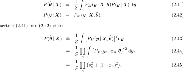
To explain this effect, let us assume we have found a set of parameters ˆθ, that is a fixpoint of the sequence (2.39,2.40) P(ˆθ|X) = 1 Z Z PM(y|X,θ)ˆ P(y|X) dy (2.41) P(y|X) = PM(y|X,ˆθ), (2.42)
Inserting (2.41) into (2.42) yields
P(ˆθ|X) =ˆ 1 Z Z PM(y|X,ˆθ) 2 dy (2.43) = 1 Z Y n Z PM(yn|xn,θ) 2 dyn (2.44) = 1 Z Y n p2n+ (1−pn)2, (2.45)
where we have used the short handpn=ˆ pM(yn= 1|xn,θ). Eq. (2.45) describes the effective
parameter distribution of self-training, whose local optima correspond to the fixpoints of the sequence (2.39,2.40).
Figure 2.8: Plot of effec-tive class purity-dependent weight of self-training. The contribution of a single datapoint to the effective
pa-rameter distribution (2.45) is plotted in Figure 2.8. As an illustrative example, let us consider two parameter vectors ˆ
θdb and ˆθu, that give the samepn for all datapoints except
one. Let us assume further that for ˆθdb, the remaining
data-point haspn= 1/2 (it is located at the decision boundary),
while for ˆθu, the remaining datapoint has pn= 0 or pn= 1
(it is unambiguously assigned to one class). In this case, the effective parameter probability (2.45) would be twice as large for the unique class assignment ˆθu than for the
unde-cided class assignment ˆθdb. The same argument holds for
all datapoints, so each datapoint that is close to the deci-sion boundary reduces the relative parameter posterior by
Chapter 2 Bayesian Learning Theory
2.5 Learning from weak labels
Supervised and semi-supervised learning consider the extreme cases of either complete class information about a datapoint (labeled) or zero class information about a datapoint (unla-beled). In practice we sometimes have a situation in between these two extremes, i. e. we have someweak information about the class of a datapoint.
The weakness of information can have different reasons. For example, the given label might be subject to statistical error, so that it only provides a prior classprobability of the corresponding datapoint. Another possible reason is that we only have aggregate informa-tion about a group (orbag) of many datapoints. In this case, though the bag label is exact, it only gives a vague information about the class of a single datapoint.
In the following we give a short overview of weak label models, focusing on bag models, since the multiple instance model is a special case of a bag model.
2.5.1 Noisy labels xn yn zn θ N
Figure 2.9: Markov net-work of learning from labels with errors.
There is no single widely accepted term to refer to the situation where the available labels are subject to errors. It has been called “noisy labels” (Natarajan, Dhillon, Raviku-mar & Tewari 2013), “errors in labels” (Buehler, Zisser-man & Everingham 2009), “uncertain labels” (Bouveyron & Girard 2009), “imperfect labels” (Tabassiana, Ghaderia & Ebrahimpourb 2012), and “ambiguous labels” (H¨ullermeier & Beringer 2005). An experimental survey of the effect of noisy labels can be found in (Nettleton, Orriols-Puig & Fornells 2010).
The common trait of these models is that the classes yn
are not observed directly, but only a third quantity zn, which is related to the class yn, is observed. The corre-sponding graphical model is shown in Figure 2.9.
Binary classification and Bernoulli model In the case of binary classification, the relation betweenyn and zn is most generally described by four parameters with one normalization constraint P(yn, zn) yn= 0 yn= 1 zn= 0 β1 β2 zn= 1 β3 β4 (2.46) β1+β2+β3+β4= 1. (2.47)
Chapter 2 Bayesian Learning Theory
P(yn|zn) yn= 0 yn= 1 zn= 0 1−βF N βF N zn= 1 βF P 1−βF P
(2.48)
where βF N is the rate of false negative labels, andβF P is the rate of false positive labels.
Often it is appropriate to setβ=βF N =βF P. Since the conditionalP(yn|zn) is a Bernoulli
distribution, we call the model (2.48) the “Bernoulli model”. In chapter 5, we propose such a Bernoulli model as an addition to the multiple instance model.
The approach to model only the conditional distribution instead of the complete joint distribution is reminiscent of the discriminative model split that we discussed in Section 2.3. But note that in this case the parametersβare assumed fixed, so parameter independence is not an additional constraint, and (2.48) is equivalent to (2.46).
xn yn znj θ N Jn
Figure 2.10: Markov net-work of learning from multiple labels.
Multiple labels When exact labels are not available, it is a natural idea to improve over a single noisy label by tak-ing multiple noisy labels (see Figure 2.10). Even when it is possible to obtain exact labels, it might be cheaper to acquire multiple noisy labels. For this reason the setting of multiple noisy labels has received considerable treatment in the literature. The model of multiple noisy labels was in-troduced by (Jin & Ghahramani 2002). Up-to-date reviews about this topic can be found in (Zhang & Zhou 2013) and (Sorower 2010).
Chapter 2 Bayesian Learning Theory xbn ybn cb θ β Nb B
Figure 2.11: Markov net-work of learning from bag labels with bag parameters β. The loop at node ybn
indicates that all {ybn}n
are pairwise connected (see text for explanation). Another form of weak labels arises if we are not given
the class information for each single datapoint, but only aggregate information about many datapoints. Each set of datapoints gives rise to a multiset – orbag – of classes, and for each bag we are given onebag label c. In this context a single datapoint is usually referred to as aninstance in order to distinguish it from its respective bag. The corresponding graphical model is shown in Figure 2.11.
The most well-known bag model seems to be the so-called multiple instance model, where the bag label is negative if
all instance labels are negative, and positive ifat least one
instance label is positive. This model is a main topic of this work, and we will discuss it in detail in the following section. Another (more informative) bag label would be the counts of instance classes within each bag. Such labels have been used for learning by (K¨uck & de Freitas 2005).
Note that the essential difference between bag models and noisy labels is that bag models allow for correlations
be-tween the instances of the same bag. Formally, the bag model factorQB does not factorize
into instances, but only into bags:
QB(Y,c,β) = Y b Qb((yb, cb,β) (2.49) 6= Y b Y n Qb((ybn, cb,β), (2.50)
where the bold symbols stand for sets of variables: Y ={ybn}bn, yb = {ybn}n, c = {cb}b.
To represent the factorization (2.49) by a the Markov network, ally-nodes on eachN-plate must be pairwise connected. We have indicated this in Figure 2.11 by a loop.
The fact that bag models do not factorize into instances makes learning difficult. We will encounter this problem in Chapter 6, when devising an algorithm for multiple instance learning.
2.5.3 Inference in bag models
When dealing with bag models, we must take into account the interaction between the classifier and the bag model. The latent instance classesydepend both on the classification model P(x, y,θ) and on the bag modelP(y, c,β). This has the consequence that the two submodels cannot be regarded as separate anymore, but they become factors QCl, QB of
the joint modelP(X,y, c,θ,β).
In this section, we derive the expressions that are needed to do inference in general bag models. To our knowledge, these expressions have not been published before. For clarity, we state the expressions for only one bag and leave out the products over bag indicesb.
Chapter 2 Bayesian Learning Theory
Let us denote the factor describing the classification model byqCland the factor describing
the bag model byQB. The joint probability of the complete model is P(X,y, c,θ,β) = 1 ZQCl(X,y,θ)QB(y, c,β) (2.51) QCl(X,y,θ) = Y n qCl(xn, yn,θ) (2.52) Z = Z QClQB dX dydcdθdβ, (2.53)
whereX ={xn}denotes the set of all feature vectors of one bag, and the partition function
Z ensures normalization.
Note that although the factors qCl and QB represent the probabilities P(xn, yn,θ) and
P(y, c,β), resp., they are not equal to the corresponding marginal probabilities of the joint model qCl 6= P(xn, yn,θ) = Z P(X,y, c,θ,β) dxm=6 ndym6=ndcdβ (2.54) QB 6= P(y, c,β) = Z P(X,y, c,θ,β) dX dθ. (2.55) This can be quite counter-intuitive, as we will discuss in Section 5.1.4 for the case of the Bernoulli bag model.
It is convenient to use a distinct symbol My for the marginal over the latent variables y
and focus on its dependence on the parameters (θ,β) and on the bag class c.
My(θ,β, c) = P(c,X,θ, β) =
Z
QB QCldy (2.56)
The parameter posteriorP(θ,β|x, c) (needed for training) and the bag class probability
P(c|X,θ, β) (needed for testing) now take on the following simple forms
P(θ, β|X, c) = R My My dθ dβ ∝ My(θ,β) (2.57) P(c|X,θ, β) = R My My dc = My(c) My(c= 0) +My(c= 1) (2.58) Note that for maximization of or sampling from the parameter posterior (2.57) it is not necessary to know the denominator (normalization constant), but for bag classification (2.58) the denominator is essential.
For discriminative bag models, the above expressions can be simplified (see Section 4.1). Since the multiple instance model is a discriminative bag model, it does not necessarily require the general expressions above. However, for the improvements and generalizations we propose in Chapters 4 and 5, the general expressions stated above are indeed necessary, and we will refer to Equations (2.56–2.58) when discussing and analyzing these models.
Chapter 3
Multiple Instance Learning
Multiple instance learning is the central topic of this work. It allows to learn from bag labels, where a negative bag label implies that all of its instances are negative, and a positive bag label implies that at least one of its instances are positive. This bag model corresponds to the setting of industrial optical inspection, where an image is labeled as negative only if it is entirely free of defects, and labeled positive if it contains at least one defect.
Multiple instance learning has originally been proposed by (Dietterich, Lathrop & Lozano-P´erez 1997) for an application of drug activity prediction. Since then it has found several other applications in image classification, text categorization, data mining, and others. It has received continued attention from the machine learning community and several algo-rithms for multiple instance learning have been proposed.
In this chapter we will give an overview of the multiple instance model, its applications, and available algorithms.
3.1 The multiple instance model
3.1.1 Model definition
The multiple instance model is actually a deterministic bag model. However, it is only useful in combination with a probabilistic classifier. Therefore, we state below both the deterministic and the probabilistic expressions.
Multiple instance bag model (deterministic) The multiple instance model relates the bag classc to the instance classesy={yn}. The informal definition is
bag negative ⇔ all instances negative
bag positive ⇔ at least one instance positive (3.1)
Formally, this is expressed most concisely as
c = max
n yn = ORn(yn) ⇐⇒ (3.2)
1−c = min
Chapter 3 Multiple Instance Learning
where c and yn are binary variables with c = 0 (or yn = 0) denoting a negative class membership and c= 1 (oryn= 1) denoting a positive class membership.
An example of a bag containing two instances is
c y2= 0 y2= 1
y1= 0 0 1
y1= 1 1 1
(3.4)
For bags containing more instance, one can imagine an N-dimensional cube where one orthant is 0 and all others are 1.
Note that the multiple instance bag model is in fact a deterministic model. If the instance classes y are known, the bag class c is determined exactly. The probabilistic nature of multiple instance learning originates solely from the probabilistic classifier.
xbn ybn cb θ N B Figure 3.1: Graphical model of multiple instance learning.
Multiple instance classification model (probabilistic) The multiple instance bag model (3.2) is always used together with a probabilistic classifier. The combined model (clas-sifier plus MI) is characterized by the y-marginal My. To
evaluate it, we first we state (3.2) as a degenerate probabil-ity distribution QMI(y, c) = δ c,max n yn , (3.5)
and we introduce the short-hand
pn = qCl(xn, yn,θ) (3.6)
In the following, we refer to pn as the “soft outputs” of the instance classifier. Now, Eq.
(2.56) evaluates as MMI(c= 0) = Y n (1−pn) = ANDn(1−pn) (3.7) MMI(c= 1) = 1− Y n (1−pn) = ORn(pn). (3.8)
SinceMMI(c= 0) +MMI(c= 1) = 1, the denominator of (2.58) is trivial and we have
P(c= 1) = 1−Y
n
(1−pn) = ORn(pn). (3.9)
We have used the notation “AND” and “OR” for probabilistic conjunction and disjunc-tion, resp. Probabilistic OR is often called “noisy-OR” in the literature. The expression (3.9) was first stated by (Maron & Lozano-P´erez 1998) and is well-known in the literature. However, the conceptual distinction between the (deterministic) label model itself and its
Chapter 3 Multiple Instance Learning
(probabilistic) combination with the classifier is usually not made.
Note that the term “multiple instance learning” is a bit misleading because actually all
bag models involve multiple instances, not just the specific model defined above. A more descriptive term would be “bag-OR model”. We point this out because the improper name has led to some confusion; for instance, (Amores 2013) uses the term “multiple instance” as referring to the class of all bag models. But since the majority of papers uses the term “multiple instance learning” according to the above definition, we adopt this term although it is somewhat misleading.
3.1.2 Model training
To get an idea of the effect of the multiple instance (MI) model on classifier training, we examine the negative log-likelihood of the model as a function of the soft outputs of the instance classifier. Comparing Equations (2.57), (3.7), and (3.7), we find
NLL−MI(p) = −log(MMI(c= 0)) = − X n log(1−pn) (3.10) NLL+MI(p) = −log (MMI(c= 1)) = −log 1− Y n (1−pn) ! , (3.11)
where (3.10) is valid for bags labeled “negative” and (3.10) is valid for bags labeled “posi-tive”. Note that the model likelihood for positive bags does not factorize, which makes MI learning hard.
To understand the behavior of the model, it is useful to separate a single instancepj in the
formulas (3.10,3.11), so that we see the effect of changing this instance’s class probability on the bag model likelihood. For negative bags this is trivial because it factorizes into instances, but for positive bags we have to take some care.
It is convenient to summarize all instances other than j in a single term p\j ={pn}n6=j.
Then we can express the complete bag’s negative log-likelihood as a function of the “re-duced” bag’s negative log-likelihood NLL(p\j) and pj:
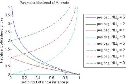
NLL−MI(pj,p\j) = −log(1−pj) + NLL−MI(p\j) (3.12) NLL+MI(pj,p\j) = −log h 1−1−pj 1−exp h NLL+MI(p\j) ii (3.13) These functions of two variables can be plotted as a set of curves, as is done in Figure 3.2. The slope of the curves characterizes the impact of a single instance on the total bag likelihood. If the slope is large, the multiple instance model will “push” the instance classifier hard to change the class assignment of that instance.
As expected, an instance’s impact is the larger the more its class probability contradicts the given bag label. For negative bags, completely positive instances (pj = 1) are forbidden
(dashed curves). For positive bags, an instance’s impact on the bag-NLL depends on the remaining instances of its bag. If one (or several) of them is positive, they have already
Chapter 3 Multiple Instance Learning
Figure 3.2: Contribution of a single instance to the negative log-likelihood of the multiple instance model. The negative log-likelihood of the “reduced” bag is denoted by NLLr =
NLL(p\j).
“justified” the positive bag label (NLL(p\j) = 0), and the class assignment for instancej
becomes irrelevant (constant cyan curve). If none of the remaining instances are positive, the positive bag label is not yet “justified” (NLL(p\j) 1), and the remaining instance is strongly pushed to a positive class assignment (solid blue curve).
3.1.3 Relation to semi-supervised learning
Multiple instance (MI) learning has some similarity with semi-supervised learning (SSL). To make this apparent, consider an asymmetric semi-supervised setting where all labeled datapoints are negative (i. e. there are no positive labels at all). Then the labeled data-points correspond to the instances from negative MI-bags, while the unlabeled datadata-points correspond to instances from positive MI-bags.
The correspondence is not exact, because the instances from positive MI bags are not really unlabeled. Instead, at least one of the instances from each positive MI-bag must be positive. This can be viewed as a constraint on the instance classes, and we will refer to this in the following as theMI-constraint.
Note that the hypothetical asymmetric semi-supervised setting above is actually ill-defined, because the best fit to the observed data (without any positive labels) is the trivial one of classifying all datapoints as negative. The only thing that prevents this degenerate solution in the multiple instance setting are the MI-constraints.
Chapter 3 Multiple Instance Learning
learning many methods that have been proposed for one of these settings has also been ap-plied to the other. Notable semi-supervised methods that are related to multiple instance learning are (K¨uck, Carbonetto & de Freitas 2004), (Goldman & Rahmani 2006), (Zhou & Xu 2007), (Leistner, Saffari, Santner & Bischof 2009), and (Zeisl, Leistner, Saffari & & Bischof 2010).
Low-density separation During training the multiple instance model, we can distinguish between two different situations. For positive bags with large negative likelihood, we say that the constraint is active, for positive bags with small negative likelihood, the MI-constraint is inactive.
The situation where the MI-constraint is inactive corresponds to semi-supervised learning. In this case, we have to adopt one of the four model assumptions of semi-supervised learning (see Section 2.4). As mentioned above, these assumptions are more or less equivalent. We find the assumption of low-density separation most intuitive.
Our algorithm described in Section 6 is based on self-training and therefore exhibits the kind of low-density separation described in Section 2.4.1.
3.2 Interpretations and variants of the multiple instance model
When the multiple instance model was first proposed (Dietterich et al. 1997), it was not stated as formally as above, but as a verbal description of the application’s requirements. Besides the above described model, there are some slightly different variants that are also plausible and correspond to the verbal description (3.1).
In this section we describe these different variants and analyze in which applications they are appropriate.
3.2.1 Standard MI (sMI): Estimate latent instance classes
To distinguish the MI model as defined in Section 3.1 from the following MI variants, we call it the “standard MI” or “sMI” model.
The main point that distinguishes the sMI model from the following MI models is the role of the instance classesy. In sMI, they are treated as latent variables that are unknown, but are explicitly estimated during training and passed as input to the instance classifier.
3.2.2 Discard non-positive instances (dMI)
Let us denote the datapoints from positive bags that are in fact negative as the “non-positive” instances. While in the standard MI model the non-positives are regarded as negative, it is also possible to discard them, so they have no effect on the instance classifier. We call this approach “dMI”.
This approach seems reasonable if there are already many negative instances from negative bags. One might consider this as the “safe” option, because we do not know for sure which
Chapter 3 Multiple Instance Learning
instances are the non-positives are never known for sure to be negative, because the MI learner might have erred.
However, discarding the non-positives has another effect: The MI learner now prefers to discard as many instances as possible and to estimate as few instances as possible as truly positive. This leaves only the most extreme instance of each positive bag, and the MI learner will place the decision boundary in the middle between the most extreme instances of the negative bags and the most extreme instances of the positive bags. In the following we will call the “most extreme” (i. e. most positive) instance of a bag as the bag’switness. The idea to discard non-positives was first proposed by (Andrews, Tsochantaridis & Hofmann 2002) for the adaption of support vector machines to multiple instance-learning. They named their implementation of dMI “MI-SVM” and their implementation of sMI “mi-SVM”. Improved versions of these algorithms have been proposed by (Gehler & Chapelle 2007), called “AW-SVM” and “AL-SVM”, resp., where the W stands for “witness” and L stands for “all labels”. We believe that a clear and ambiguous terminology is needed to distinguish between the two models, irrespective of algorithmic details, so we propose the terminology “sMI” and “dMI” as stated in the headlines.
Formal statement of dMI-model Proceeding to a formal statement of the dMI-model, we label the negative class by y=−1 and introduce a third instance “class” y= 0 that labels discarded instances. The bag model of dMI is represented by (cf. Eq. (3.2))
QdMI(c=−1,y) = ( 1 if maxnyn=−1 0 otherwise (3.14) QdMI(c= 1,y) = (
1 if (maxnyn= 1) AND (minnyn>−1).
0 otherwise (3.15)
An example of a bag containing two instances is the following (This might be compared to the example in Section 4.1.2):
QdMI(c=−1,y) y2=−1 y2= 0 y2= 1 y1=−1 1 0 0 y1= 0 0 0 0 y1= 1 0 0 0 (3.16) QdMI(c= 1,y) y2=−1 y2= 0 y2= 1 y1=−1 0 0 0 y1= 0 0 0 1 y1= 1 0 1 1 (3.17)
Chapter 3 Multiple Instance Learning xn0 yn0 cb θ xn00 0 Nb0 Nb00 B
Figure 3.3: Markov net-work of dMI-model (multi-ple instance with discarding of non-positives).
Next we need to define how “discarded” instances (yn= 0) are treated by the instance classifier. From a practical point of view, one can just leave the discarded points out of the corresponding factor (cf. Eq. (2.52))
QCl(X,y,θ) = Y
n:yn6=0
qCl(xn, yn,θ) (3.18)
The problem with this approach is that the factor (2.52) is in fact determined by the laws of Bayesian inference, and we are not allowed to change it at will. Actually, our newly defined factor (3.20) corresponds to a different graphical model, shown in Figure 3.3. Note that the discarded points xn00have no connection to any other nodes. So during
train-ing, one actually does not only infer the values of parameters and latent variables, but the model structure itself is
flex-ible. There are methods that can learn the model structure (Daly, Shen & Aitken 2011), but this is actually a bit over the top for the model above.
Instead, it is much easier to introduce another factorqCl0 (x, y,θ) than to change the model structure. qCl0 (xn, yn,θ) = ( 1 qCl(xn,yn,θ) ifyn= 0 0 otherwise (3.19) QCl(X,y,θ) = Y n qCl(xn, yn,θ)qCl0 (xn, yn,θ) (3.20)
Note thatQCl as defined above is not normalized, so care must be taken when interpreting
it as a classification probability.
Testing the dMI model A change of model affects both training and testing. Since dMI discards instances during training, the same is allowed during testing. This corresponds to the “threshold” method (cf. Section 4.2.2).
One-class learning of witnesses (wMI) In the original multiple instance application of drug activity prediction, it is known that the positive region in feature space is very small. In this case it is plausible to try and find the smallest positive region that explains all positive bags. Indeed, this is the underlying idea of the first proposed MI algorithms “APR” and “diverse density” (see Section 3.4).
This approach is actually a form of one-class learning of the positive bags’ witnesses (most positive points of each bag). In this approach the negative bags are used merely to identify the witnesses. Once the witnesses are known, the decision boundary is fitted around them as tight as possible without taking into account the negative points anymore.
Chapter 3 Multiple Instance Learning
Figure 3.4: Illustration of sesqui-class learning. Solid lines: Observed densities of positive and negative bags. Dashed: True positive density.
3.2.3 Sesqui-class learning (SCL)
Sesqui-class learning is based on the generative approach, i. e. the classification model is divided into class densities P(x|y,θ) and a class prior P(y|π) (see Section 2.3)
P(x, y,θ, π) = P(x|y,θ)P(y|π)P(θ)P(π) (3.21) In the MI setting we cannot observe these densities directly because the instance classesyn
are latent. We only know the bag classc, and according to the MI model the corresponding densities can be written as
P(x|c= 0) = P(x|y= 0) (3.22)
P(x|c= 1) = αP(x|y= 1) + (1−α)P(x|y= 0) 0< α <1. (3.23) Negative bags contain only negative instances, but positive bags contain both positive and negative instances, so their combined density is a mixture of the true positive and true negative densities. The observed bag densities and the true instance class densities are illustrated in Figure 3.4.
The mixture parameterα is given by the bag sizes and the class prior. Let (N+, N−) be
the numbers of instances from positive and negative bags, resp. Then
P(y= 1|π) = π = αN + N++N− (3.24) α = π 1 +N − N+ (3.25)
Since the bag sizes are known, estimation of the mixture parameterα and the class priorπ