Measuring and predicting the effects of time-variable
exposure of pesticides on populations of green algae:
Combination of flow-through studies and ecological modelling as an
innovative tool for refined risk assessments
Von der Fakultät für Mathematik, Informatik und Naturwissenschaften der RWTH
Aachen University zur Erlangung des akademischen Grades eines Doktors der
Naturwissenschaften genehmigte Dissertation
vorgelegt von
Diplom-Bioinformatiker (FH)
Denis Weber
aus Frankfurt am Main
Berichter: apl. Professor Dr. rer. nat. Hans Toni Ratte
Universitätsprofessor Dr. rer. nat. Andreas Schäffer
Tag der mündlichen Prüfung: 14. September 2012
"As far as the laws of mathematics refer to reality, they
are not certain; as far as they are certain, they do not
refer to reality."
Albert Einstein
Acknowledgements
I am heartily thankful to my supervisor, Prof. Dr. Hans Toni Ratte, whose encouragement, guidance, support and patience from the initial to the final level enabled me to realize this thesis. It was an honor for me to work under his excellent supervision.
I owe my most sincere gratitude to Dr. Michael Dorgerloh for his trust, confidence and enthu-siasm to support the realization of the flow-through experiments. He shared his excellent knowledge and experiences with me and his intensive mentoring and on-the-spot support of the experiments made this work possible.
I owe my deepest gratitude to Dr. Dieter Schäfer for his important support throughout this work and for his detailed review, constructive criticism and excellent advice during the prepa-ration of this thesis.
I wish to express my warm and sincere thanks to Dr. Gerald Reinken for his friendship, per-sonal favors and for accommodation during the time-intensive laboratory experiments. Our extensive discussions around my work, his understanding, encouraging and personal guid-ance have been of great value for me.
I would like to show my gratitude to my Dr. Thomas Preuss for his detailed and constructive comments and valuable advices, for his guidance in scientific questions, and for his im-portant support throughout this work.
I am very grateful to Dr. Fred Heimbach for his untiring help and intensive talks during my difficult moments.
My sincere thanks are due to Dr. Eric Bruns and Dr. Gerhard Görlitz for their support of the project, their patience and helpful advices.
I wish to thank Dr. Klaus Hammel for his help and supervision in solving mathematical and modelling problems. His kind support and guidance have been of great value for this work. I also wish to thank Dr. Robin Sur and Dr. Barbara Koch for our valuable discussions and their advices throughout this project.
I wish to extend my warmest thanks to all those who have helped me in the work group of Aquatic Ecology and Ecotoxicology at the RWTH Aachen University, especially Birgitta Gof-fart, Katrin Liedtjens, André Gergs, Hanna Maes, Helga von Lochow, Stefanie Uecker and Brigitte Thiede.
My special thanks go to Kristine Holz and Prof. Dr. Ingolf Schuphan.
I am grateful to the laboratory team at Bayer CropScience AG, Department of Ecotoxicology, especially to Oliver Kielack for his support during the flow-through experiments and to Heiko Spauszus, Olaf Wüstner and Thomas Riebschläger for their technical support and advices. I finally wish to thank Ernst Bühler-Koch for drawing the 3D-model of the flow-through sys-tem.
T
ABLE OFC
ONTENTS1. INTRODUCTION ... 1
2. BACKGROUND ... 3
2.1 Preface ... 3
2.2 The European Standard Risk Assessment for Pesticides ... 3
2.3 The FOCUS Exposure Assessment ... 5
2.3.1 A Tiered Approach in Four Steps ... 5
2.3.2 The FOCUS Scenarios ... 7
2.3.3 The FOCUS Water Body Systems ... 8
2.3.4 The FOCUS Step 3 Modelling Concept ... 10
2.3.5 Time-Variable Exposure Patterns ... 12
2.4 Higher-Tier Risk Assessments ... 14
2.4.1 Overview ... 14
2.4.2 Mesocosms - Aquatic Model Ecosystems ... 15
2.4.3 Models in Ecology and Risk Assessment ... 17
3. PROBLEM DESCRIPTION ...20
4. OBJECTIVES AND CONCEPTUAL APPROACH ...22
4.1 Objectives ... 22
4.2 Conceptual Approach ... 24
5. MATERIAL AND METHODS ...26
5.1 Test Organisms... 26
5.1.1 Selection of Algae Species ... 26
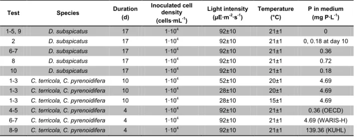
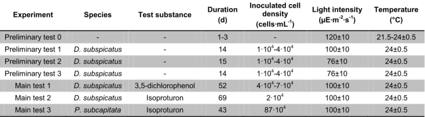
5.1.2 D. subspicatus ... 28 5.1.3 P. subcapitata ... 29 5.1.4 C. terricola ... 30 5.1.5 C. pyrenoidifera ... 32 5.1.6 Culture Conditions ... 34 5.1.7 Stock Cultivation ... 35 5.1.8 Rating Curves ... 36 5.2 Test Substances ... 37 5.2.1 Isoproturon ... 37 5.2.2 3,5-dichlorophenol ... 39
5.3 Static Algae Tests ... 40
5.3.1 Growth Conditions ... 40
5.3.2 Capacity ... 43
5.3.3 Phosphate-Uptake ... 46
5.3.4 Competition ... 50
5.3.5 Growth Inhibition ... 54
5.4 Flow-through Algae Tests ... 56
5.4.1 Background ... 56
5.4.2 Preparation and Setup ... 57
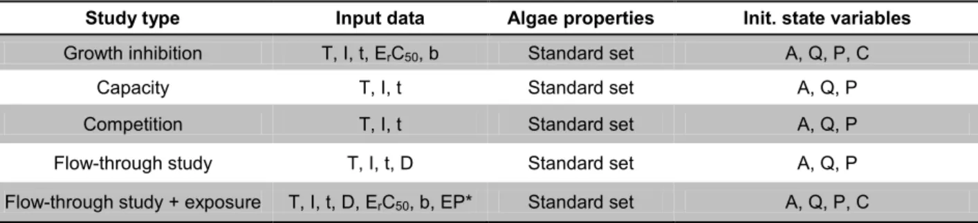
6. MODEL DEVELOPMENT ...60
6.1 A Simple Algae Model ... 60
6.1.1 Description and Conceptual Model... 61
6.1.2 State Variables and Parameters ... 62
6.1.3 Initialization ... 63
6.2 Submodels ... 64
6.2.1 Basic Growth Models ... 64
6.2.2 Algae Population Growth ... 66
6.2.3 Light Dependence ... 67
6.2.4 Temperature Dependence ... 68
6.2.5 Nutrient Dependence ... 69
6.2.6 Internal P Concentration in Algae Cells ... 70
6.2.7 External P Reservoir ... 71
6.2.8 Effect of a Chemical Stressor ... 72
6.2.9 Single-First-Order Kinetics ... 73
6.2.10 The SAM-X Model ... 74
6.3 Implementation ... 75
6.3.1 Stiffness ... 75
6.3.2 Numerical Solver ... 75
6.4 Parameterization ... 76
6.4.1 Overview of Reported Parameter Values ... 77
6.5 Sensitivity Analysis ... 78
6.5.1 Description ... 78
6.5.2 Variation of µmax and qmin ... 79
6.5.3 Variation of qmax, vmax and ks ... 80
6.5.4 Variation of D and R0 ... 82
6.5.5 Summary and Conclusion ... 83
6.6 Standardized Parameter Sets ... 85
6.7 Model Setup for Simulations ... 86
7. THE ALGAE FLOW-THROUGH SYSTEM ...88
7.1 The Chemostat Principle ... 88
7.1.1 Technical Description of the Flow-through System ... 89
7.2 Factors of Influence for Growth in Chemostats ... 92
7.2.1 Variations of the Initial Cell Density ... 92
7.2.2 Variations of the Dilution Rate ... 93
7.2.3 Variations of the Maximum Growth Rate ... 93
7.2.4 Variations of the Inflowing Nutrient Concentration ... 93
7.2.5 Simultaneous Variations of Factors of Influence for Growth ... 94
7.3 Interpretation of Flow-through Experiments ... 96
7.3.1 The Five Phases of an Exposure Event ... 96
7.3.2 The Usage of a ‘Static’ ErC50 under Flow-through Conditions ... 97
7.3.3 The Dependency of the Duration of Exposure Events on the Effects on Algae ... 99
8. RESULTS ... 102
8.1 The Variance in Algae Growth Inhibition Studies ... 102
8.2 Static Algae Tests ... 107
8.2.1 Growth Conditions ... 107
8.2.2 Capacity ... 111
8.2.3 Phosphate-Uptake ... 119
8.2.4 Competition ... 127
8.2.5 Growth Inhibition ... 132
8.3 Flow-through Algae Tests ... 138
8.3.1 Preliminary-Tests ... 138
8.3.2 Test with 3,5-dichlorophenol ... 141
8.3.3 Tests with Isoproturon ... 144
8.4 Validation of Parameter Sets ... 155
8.5 Extrapolation Scenario ... 158
8.5.1 Purpose ... 158
8.5.2 Toxicity Data ... 158
8.5.3 Exposure Pattern ... 159
8.5.4 Setup for the Modelling Approach ... 159
8.5.5 Model Predictions ... 160
8.5.6 Modified Model Predictions ... 161
8.5.7 Discussion ... 162
9. DISCUSSION AND FINAL CONCLUSIONS ... 163
10. BIBLIOGRAPHY ... 169
11. APPENDIX ... 184
11.1 Abbreviations and Symbols ... 184
11.2 Raw Data ... 185
11.2.1 Growth Conditions Tests ... 185
11.2.2 Capacity Tests ... 186
11.2.3 Competition Tests ... 190
11.2.4 Growth Inhibition Tests ... 193
11.3 Literature Sources for Parameter Values ... 194
11.4 Algae Growth Media ... 197
11.4.1 OECD 201 culture medium ... 197
11.4.2 WARIS-H culture medium ... 198
11.4.3 KUHL culture medium... 200
11.5 Photosynthesis Inhibiting Herbicides ... 201
11.6 Approach to Combine Flow-through Tests and Modelling ... 202
11.7 Materials and Software ... 204
SUMMARY ... 205
L
IST OFF
IGURESFigure 2-1: Tiered approach in FOCUS exposure assessment ... 6
Figure 2-2: Location of the ten FOCUS surface water scenarios across Europe ... 7
Figure 2-3: FOCUS ditch scenario ... 8
Figure 2-4: FOCUS pond scenario ... 8
Figure 2-5: FOCUS stream scenario ... 9
Figure 2-6: FOCUS Step 3 modelling concept ... 10
Figure 2-7: FOCUS exposure pattern, drainage scenario, water body: ditch ... 13
Figure 2-8: FOCUS exposure pattern, drainage scenario, water body: pond ... 13
Figure 2-9: FOCUS exposure pattern, runoff scenario, water body: stream ... 13
Figure 3-1: Problem description scheme ... 20
Figure 3-2: FOCUS calculation for a pesticide in a runoff scenario ... 21
Figure 4-1: Conceptual approach ... 23
Figure 5-1: Pictures of D. subspicatus ... 28
Figure 5-2: Pictures of P. subcapitata ... 29
Figure 5-3: Pictures of Chlamydomonasspec. ... 30
Figure 5-4: Cell and life cycle of Chlamydomonas spec. ... 31
Figure 5-5: Pictures of Cryptomonas spec. ... 32
Figure 5-6: Cell morphology of Cryptomonas spec. ... 33
Figure 5-7: Rating curve D. subspicatus ... 36
Figure 5-8: Rating curve P. subcapitata ... 36
Figure 5-9: Rating curve C. terricola ... 36
Figure 5-10: Rating curve C. pyrenoidifera ... 36
Figure 5-11: Annual dynamics of light and temperature ... 40
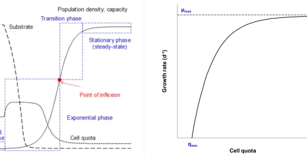
Figure 5-12: Algae population growth dynamics ... 44
Figure 5-13: Asymptotic behavior of the cell quota model ... 44
Figure 5-14: Rating curves with phosphate standard (tests with D. subspicatus) ... 47
Figure 5-15: Rating curves with phosphate standard (tests with C. pyrenoidifera) ... 47
Figure 5-16: Growth of P aurelia and P. caudatum in separate and mixed cultures. ... 50
Figure 5-17: Growth phases of algae populations under controlled culture conditions ... 58
Figure 6-1: Model concept of SAM-X ... 61
Figure 6-2: One solution of the logistic differential equation ... 65
Figure 6-3: Example f(I) response curve ... 67
Figure 6-4: Example f(T) response curve ... 68
Figure 6-5: Example f(Q) response curve ... 69
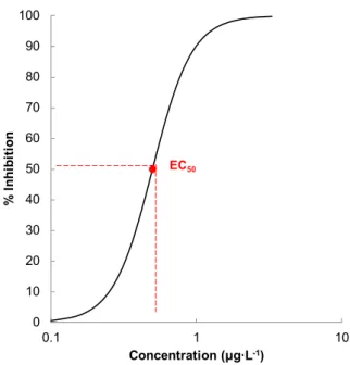
Figure 6-6: Example of a log-logistic concentration-effect curve ... 72
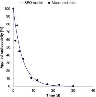
Figure 6-7: Example data and corresponding SFO decline curve ... 73
Figure 6-8: Surface plot of variation of µmax ... 79
Figure 6-9: Surface plot of variation of qmin ... 79
Figure 6-10: Surface plot of variation of qmax ... 80
Figure 6-11: Surface plot of variation of vmax ... 80
Figure 6-12: Surface plot of variation of ks ... 81
Figure 6-13: Surface plot of variation of D ... 82
Figure 6-14: Surface plot of variation of R0 ... 82
Figure 6-15: Maximum change of biomass by ±30% variation of different parameters ... 83
Figure 7-1: Flow-through system under experimental conditions ... 90
Figure 7-3: 3D model of the flow-through system ... 91
Figure 7-4: Population dynamics with different initial cell densities ... 95
Figure 7-5: Population dynamics with different dilution rates ... 95
Figure 7-6: Population dynamics with given µmax and varied dilution rate from day 25 ... 95
Figure 7-7: Population dynamics with different dilution rates and varied µmax from day 25 ... 95
Figure 7-8: Population dynamics with different nutrient inflows (R0) ... 95
Figure 7-9: Population dynamics with time-variable nutrient inflows (R0) ... 95
Figure 7-10: Illustration of the five phases occuring in a flow-through experiment ... 96
Figure 7-11: Effects of a constant ErC50 exposure on a population ... 98
Figure 7-12: Population exposed to ErC50 peaks of different duration ... 99
Figure 7-13: Concentration-effect curves with different slope values ... 100
Figure 7-14: Population in a flow-through system with different slope values ... 101
Figure 8-1: Variance in 72 h growth inhibition tests ... 103
Figure 8-2: Temperature and light intensities plotted vs. 72 h growth rate ... 103
Figure 8-3: Surface fit to data of growth rate vs. light and temperature ... 104
Figure 8-4: Contour fit to data of growth rate vs. light and temperature... 104
Figure 8-5: Control measurements of 202 growth inhibition studies ... 105
Figure 8-6: Simulations of 72 h growth with default parameter settings ... 106
Figure 8-7: Cell densities of D. subspicatus grown in starving cultures ... 107
Figure 8-8: Cell densities of D. subspicatus at three different nutrient conditions ... 107
Figure 8-9: Growth of C. terricola in different nutrient media ... 108
Figure 8-10: Overview of 72 h growth rates (d-1) ... 108
Figure 8-11: Growth of C. pyrenoidifera in different nutrient media ... 108
Figure 8-12: Cell densities of C. terricola grown at different environmental conditions ... 109
Figure 8-13: Cell densities of C. pyrenoidifera at different environmental conditions ... 109
Figure 8-14: Capacity tests, measured population dynamics, D. subspicatus ... 113
Figure 8-15: Capacity tests, sectional growth rates, D. subspicatus... 113
Figure 8-16: Capacity tests, measured population dynamics, P. subcapitata ... 113
Figure 8-17: Capacity tests, sectional growth rates, P. subcapitata ... 113
Figure 8-18: Capacity tests, measured population dynamics, C. terricola ... 114
Figure 8-19: Capacity tests, sectional growth rates, C. terricola ... 114
Figure 8-20: Capacity tests, measured population dynamics, C. pyrenoidifera ... 114
Figure 8-21: Capacity tests, sectional growth rates, C. pyrenoidifera ... 114
Figure 8-22: Capacity tests, modelled population dynamics, D. subspicatus ... 116
Figure 8-23: Capacity tests, calculated vs. observed, D. subspicatus ... 116
Figure 8-24: Capacity tests, modelled population dynamics, P. subcapitata ... 116
Figure 8-25: Capacity tests, calculated vs. observed, P. subcapitata ... 116
Figure 8-26: Capacity tests, modelled population dynamics, C. terricola ... 117
Figure 8-27: Capacity tests, calculated vs. observed, C. terricola ... 117
Figure 8-28: Capacity tests, modelled population dynamics, C. pyrenoidifera ... 117
Figure 8-29: Capacity tests, calculated vs. observed, C. pyrenoidifera ... 117
Figure 8-30: Overview of determined population capacities ... 118
Figure 8-31: P-uptake test 1, cell densities ... 121
Figure 8-32: P-uptake test 2, cell densities ... 121
Figure 8-33: P-uptake test 1, P in biomass ... 121
Figure 8-34: P-uptake test 2, P in biomass ... 121
Figure 8-35: P-uptake test 1, P in medium ... 121
Figure 8-36: P-uptake test 2, P in medium ... 121
Figure 8-38: P-uptake test 4, cell densities ... 122
Figure 8-39: P-uptake test 3, P in biomass ... 122
Figure 8-40: P-uptake test 4, P in biomass ... 122
Figure 8-41: P-uptake test 3, P in medium ... 122
Figure 8-42: P-uptake test 4, P in medium ... 122
Figure 8-43: Long-term P-uptake, cell densities, P in medium, D. subspicatus ... 124
Figure 8-44: Long-term P-uptake, P in biomass, D. subspicatus ... 124
Figure 8-45: Long-term P-uptake, cell densities, P in medium, P. subcapitata ... 124
Figure 8-46: Long-term P-uptake, P in biomass, P. subcapitata ... 124
Figure 8-47: Long-term P-uptake, cell densities, P in medium, C. terricola ... 125
Figure 8-48: Long-term P-uptake, P in biomass, C. terricola ... 125
Figure 8-49: Long-term P-uptake, cell densities, P in medium, C. pyrenoidifera ... 125
Figure 8-50: Long-term P-uptake, P in biomass, C. pyrenoidifera ... 125
Figure 8-51: D. subspicatusvs.P. subcapitata,1:1 ratio, cell densities ... 128
Figure 8-52: D. subspicatusvs.P. subcapitata,1:1 ratio, calculated vs. observed ... 128
Figure 8-53: D. subspicatusvs.P. subcapitata, 1:3 ratio, cell densities ... 128
Figure 8-54: D. subspicatusvs.P. subcapitata, 1:3 ratio, calculated vs. observed ... 128
Figure 8-55: D. subspicatusvs.P. subcapitata, 3:1 ratio, cell densities ... 128
Figure 8-56: D. subspicatusvs.P. subcapitata, 3:1 ratio, calculated vs. observed ... 128
Figure 8-57: C. terricola vs. C. pyrenoidifera, 1:1 ratio, cell densities ... 130
Figure 8-58: C. terricola vs. C. pyrenoidifera, 1:1 ratio, calculated vs. observed ... 130
Figure 8-59: C. terricola vs. C. pyrenoidifera, 1:3 ratio, cell densities ... 130
Figure 8-60: C. terricola vs. C. pyrenoidifera, 1:3 ratio, calculated vs. observed ... 130
Figure 8-61: C. terricola vs. C. pyrenoidifera, 3:1 ratio, cell densities ... 130
Figure 8-62: C. terricola vs. C. pyrenoidifera, 3:1 ratio, calculated vs. observed ... 130
Figure 8-63: ErC50 values with 95% confidence limits for isoproturon... 132
Figure 8-64: Concentration-effect curve, test 1, D. subspicatus ... 133
Figure 8-65: Concentration-effect curve, re-evaluated test (Hoechst), D. subspicatus ... 133
Figure 8-66: Concentration-effect curve, test 2, P. subcapitata ... 133
Figure 8-67: Concentration-effect curve, test 3, C. terricola (1) ... 133
Figure 8-68: Concentration-effect curve, test 4, C.terricola (2) ... 133
Figure 8-69: Concentration-effect curve, test 5, C. pyrenoidifera ... 133
Figure 8-70: Growth inhibition test 1, cell densities, D. subspicatus ... 135
Figure 8-71: Growth inhibition test 1, calculated vs. observed ... 135
Figure 8-72: Growth inhibition test (Hoechst), cell densities, D. subspicatus ... 135
Figure 8-73: Growth inhibition test (Hoechst), calculated vs. observed ... 135
Figure 8-74: Growth inhibition test 2, cell densities, P. subcapitata ... 135
Figure 8-75: Growth inhibition test 2, calculated vs. observed ... 135
Figure 8-76: Growth inhibition test 3, cell densities, C. terricola ... 136
Figure 8-77: Growth inhibition test 3, calculated vs. observed, C. terricola ... 136
Figure 8-78: Growth inhibition test 4, cell densities, C. terricola ... 136
Figure 8-79: Growth inhibition test 4, calculated vs. observed, C. terricola ... 136
Figure 8-80: Growth inhibition test 5, cell densities, C. pyrenoidifera ... 136
Figure 8-81: Growth inhibition test 5, calculated vs. observed, C. pyrenoidifera ... 136
Figure 8-82: Test of flow rate accuracy of solenoid pumps ... 139
Figure 8-83: Test of temperature stability in the reactor system ... 139
Figure 8-84: Preliminary flow-through tests, measured cell densities ... 139
Figure 8-85: Preliminary flow-through tests, modelled cell densities ... 139
Figure 8-87: Reproducibility of flow-through main test 1 ... 143
Figure 8-88: Modification of the FOCUS exposure pattern for isoproturon ... 144
Figure 8-89: Exposure pattern in flow-through main test 2 (D. subspicatus) ... 145
Figure 8-90: Exposure pattern in flow-through main test 3 (P. subcapitata) ... 145
Figure 8-91: Flow-through main test 2 with D. subspicatus exposed to isoproturon ... 150
Figure 8-92: Flow-through main test 3 with P. subcapitata exposed to isoproturon (A) ... 151
Figure 8-93: Flow-through main test 3 with P. subcapitata exposed to isoproturon (B) ... 152
Figure 8-94: Predicted vs. observed, capacity tests, D. subspicatus and P. subcapitata ... 157
Figure 8-95: Predicted vs. observed, capacity tests, C. terricola and C. pyrenoidifera ... 157
Figure 8-96: Predicted vs. observed, growth inhibition tests 1-2 ... 157
Figure 8-97: Predicted vs. observed, growth inhibition tests 3-5 ... 157
Figure 8-98: Predicted vs. observed, flow-through main tests, D. subspicatus ... 157
Figure 8-99: Predicted vs. observed, flow-through main tests, P. subcapitata ... 157
Figure 8-100: Concentration-effect curves, P. subcapitata, herbicide F ... 158
Figure 8-101: Modification of the calculated FOCUS exposure pattern for herbicide F... 159
Figure 8-102: Predicted population dynamics with FOCUS exposure to herbicide F ... 160
Figure 8-103: Predicted population dynamics with modified exposure to herbicide F ... 161
Figure 9-1 Combined approach of experimental studies and ecological modelling ... 167
L
IST OFT
ABLESTable 2-1: FOCUS surface water scenarios with associated water bodies and entry routes ... 7
Table 5-1: Phylum of Desmodesmus ... 28
Table 5-2: Phylum of Selenastrum ... 29
Table 5-3: Phylum of Chlamydomonas ... 30
Table 5-4: Phylum of Cryptomonas ... 32
Table 5-5: Physico-chemical properties of isoproturon ... 37
Table 5-6: Physico-chemical properties of 3,5-dichlorophenol ... 39
Table 5-7: Overview of performed growth condition experiments ... 42
Table 5-8: Overview of performed capacity experiments ... 45
Table 5-9: Overview of performed short-term P-uptake experiments ... 48
Table 5-10: Overview of performed competition experiments ... 53
Table 5-11: Overview of performed growth inhibition experiments ... 55
Table 5-12: Overview of performed flow-through experiments ... 57
Table 6-1: Physiological properties of the algae species and model parameter ... 62
Table 6-2: Environmental variables ... 62
Table 6-3: State variables of the model, additional equations and definitions ... 62
Table 6-4: Overview of input parameter for simulations of different study types ... 63
Table 6-5: Ranges of parameter values obtained from literature ... 77
Table 6-6: Standard parameter sets of the four different algae species ... 85
Table 6-7: Setup of state variables for simulations ... 86
Table 6-8: Setup for modelling based on experimental boundary conditions (1) ... 86
Table 6-9: Setup for modelling based on experimental boundary conditions (2) ... 87
Table 8-1: Variance in growth inhibition studies, D. subspicatus and P. subcapitata ... 103
Table 8-2: Determined maximum growth rates and population capacities ... 112
Table 8-3: Experimentally determined parameter values ... 120
Table 8-4: Isoproturon ErC50 values with confidence limits and slopes... 134
Table 8-5: Goodness of fit statistics ... 156
Table 8-6: ErC50 values with 95% confidence limits P. subcapitata, herbicide F ... 158
Table 8-7: Setup for model prediction of flow-through experiment with herbicide F ... 159
Table 11-1: D. subspicatus growth condition tests ... 185
Table 11-2: C. terricola and C. pyrenoidifera growth condition tests ... 185
Table 11-3: C. terricola and C. pyrenoidifera culture media tests ... 185
Table 11-4: D. subspicatus capacity tests 1-5 ... 186
Table 11-5: D. subspicatus capacity tests 6-7 ... 186
Table 11-6: P. subcapitata capacity tests 1-5 ... 187
Table 11-7: P. subcapitata capacity tests 6-7 ... 187
Table 11-8: C. terricola capacity tests 1-5 ... 188
Table 11-9: C. terricola capacity tests 6-7 ... 188
Table 11-10: C. pyrenoidifera capacity tests 1-5 ... 189
Table 11-11: C. pyrenoidifera capacity tests 6-7 ... 189
Table 11-12: Competition test 1-3 with initial cell ratio 1:1 ... 190
Table 11-13: Competition test 1-3 with initial cell ratio 1:3 ... 190
Table 11-14: Competition test 1-3 with initial cell ratio 3:1 ... 191
Table 11-15: Competition test 4-6 with initial cell ratio 1:1 ... 192
Table 11-16: Competition test 4-6 with initial cell ratio 1:3 ... 192
Table 11-17: Competition test 4-5 with initial cell ratio 3:1 ... 192
Table 11-18: Growth inhibition test 1 with isoproturon ... 193
Table 11-19: Growth inhibition test 2 with isoproturon ... 193
Table 11-21: Growth inhibition test 4 with isoproturon ... 193
Table 11-22: Growth inhibition test 5 with isoproturon ... 193
Table 11-23: Parameter values for cell volumes ... 194
Table 11-24: Parameter values for µmax ... 194
Table 11-25: Parameter values for Topt, Tmin and Tmax ... 195
Table 11-26: Parameter values for ks ... 195
Table 11-27: Parameter values for qmin and qmax... 196
Table 11-28: Parameter values for vmax and mmax ... 196
Table 11-29: Recipe for OECD 201 nutrient medium... 197
Table 11-30: Recipe for WARIS-H nutrient medium ... 198
Introduction 1
1. Introduction
At present, the application of pesticides in agriculture helps to secure the world wide food supply. The use of pesticides leads to an increased harvest per hectare as well as a reduced risk of crop losses or total crop failure. An unintended side effect of pesticide use is the harm of non-target organisms and their surrounding environment. The areas adjacent to agricul-tural fields including terrestrial, aerial, and aquatic habitats are of interest for protection. Aquatic ecosystems (e.g. ponds, ditches, streams and creeks) in agricultural areas and their inhabitants are potentially affected by pesticides and their metabolites. The toxicants can enter the aquatic environment via drift, runoff or drainage. In aquatic ecosystems the role of non-target species is important, e.g. algae as primary producers at the lowest trophic level control the nutrient cycle and water quality. An environmental risk assessment is therefore necessary to evaluate exposure and effects (SETAC 1997).
Governmental authorities have set protection criteria to prevent aquatic organisms to be en-dangered by pesticides (EC 1991; Newman and Unger 2003; Brock et al. 2006). The Euro-pean Union (EU) Council Directive 91/414 EEC is a regulatory framework that relates to the registration of pesticides in the EU (EC 1991 and 1995). Protection goals, data requirements for aquatic risk assessments and approaches for a risk characterization of the active sub-stances to be registered are considered in this directive. Due to the risk that pesticides pose to aquatic ecosystems and aquatic non-target organisms, extensive laboratory toxicity stud-ies and ERAs are required before a product can be registered in the EU. The aquatic toxicity tests include standardized experiments with aquatic plants (algae, Lemna), aquatic inverte-brates (Daphnia), and fish, and for all tested organisms toxicity endpoints are determined for later use in risk assessment (EC 1996, 1997 and 2002a; Brock et al. 2000a and 2000b). In these tests standardized and simplified exposure patterns are simulated, typically a single peak exposure in a static water body, or a constant exposure situation.
The input and the fate of pesticides in aquatic environments are calculated by mechanistic exposure models (FOCUS 2003). Exposure modelling is a regulatory standard determined by the Council Directive 91/414 and is compulsory in the risk assessment of pesticides. These models provide Predicted Environmental Concentrations in common surface water bodies (PECSW). The model calculations typically show profiles of time-variable exposure. The PECSW values are compared to the toxicity endpoints from the laboratory studies based on simple exposure assumptions.
Relating the results of these standard tests to time-variable and multiple pulsed exposure patterns is only possible by gross simplifications and the use of overly conservative
worst-case assumptions (Reinert et al. 2002). Some approaches how to evaluate pulsed exposure and how to consider it in risk assessments were proposed by e.g. Boesten et al. (2007) and the ELINK workshop (Brock et al. 2007). These concepts also include suggestions how to generalize exposure regimes for ditches, streams and ponds in order to ease the comparison with the exposure profiles of aquatic toxicity tests. This requires the identification of key characteristics of the exposure patterns (e.g. peak height, duration and interval between peaks). Population-level effects and time-to-recovery after time-variable exposure are as-pects of increasing importance. Knowledge about the responses of aquatic organisms (e.g.
green algae) to time-variable exposure needs to be gained for more realistic, but still con-servative risk assessments.
Out of the multitude of interactions of pesticides and non-target species, the example of herbicides and algae was chosen. This work presents the results of an approach to combine ecotoxicological experiments and population modelling to assess effects of pulsed exposure on algae.
Preface
Background 3
2. Background
2.1 Preface
The following background chapters provide an overview of the European Standard Risk As-sessment for plant protection products. Particularly with regard to the area of fate and expo-sure of pesticides in aquatic environments, the mandatory expoexpo-sure simulation models, their underlying principles and assumptions, as well as the problems of interpretation of the model results within the ecotoxicological risk assessment are described. The main focus of this in-troductory overview lies on the exposure and risk assessment on European level; national specific requirements are not considered here. The stepwise approach in the exposure as-sessment is explained and therefore, a description of the simulation models that calculate the fate of chemical toxicants in surface waters across Europe is given. In particular, the third step of the exposure assessment is introduced in detail due to its importance in the risk as-sessment. Examples of model outcomes are presented and explained, the complexity of the simulation results is illustrated and the problems related to the interpretation of the results are described.
2.2 The European Standard Risk Assessment for Pesticides
The regulatory risk assessment for aquatic non-target organisms is a comparison of predict-ed environmental concentrations in surface waters with toxicity data. The PECSW are esti-mated by using exposure models which calculate the fate of chemicals in surface water bod-ies (e.g. the FOCUS TOXSWA1 model). The model calculations are based on realistic worst-case exposure scenarios defined by the FOCUS group (FOCUS 2003). These FOCUS sce-narios represent agricultural conditions and different water bodies within the EU. They reflect that aquatic exposure is often characterized by multiple peaks of variable height and dura-tion, driven by spray drift inputs as well as runoff and drain flow events.
For each compound, important toxicity parameters are determined in ecotoxicological labora-tory studies, which need to be performed according to specific guidelines provided by the OECD2 (e.g. algae growth inhibition tests according to OECD guideline 201; OECD 2006). These standard toxicity studies generate data such as the No-Observed Effect Concentration (NOEC), the concentration causing 50% inhibition of the algae growth rate (ErC50) and the concentration causing 50% lethality (LC50) of fish or Daphnia. These endpoints are
1TOXic substances in Surface WAters
ry for the aquatic risk assessment. These data are further on used to assess the potential risks for representative aquatic non-target organisms which are exposed to a pesticide con-centration corresponding to the calculated PECSW.
Conservatively, as a worst-case approach for the short-term assessment, the lowest value of the acute toxicity data (LC/EC50) for aquatic organisms (plants, invertebrates and fish) is re-lated to the calcure-lated maximum PECSW and the Toxicity Exposure Ratio (TER) is calculated. The long-term assessment is performed by relating a time-weighted average3 (TWA) concen-tration to chronic effect data for the same aquatic organisms. The various TER values are then compared with regulatory required uncertainty factors (safety margins), typically 10 for chronic and 100 for acute data.
The safe use of a compound is given if the TER ≥ 10 for chronic and the TER ≥ 100 for acute toxicity is achieved. If the product passes these triggers, no further exposure assessment is necessary. In case that no safe use was attained during the standard risk assessment, more detailed data relating to environmental exposure or hazard may be required to clarify the environmental risk. Such data is generated within the higher-tier risk assessment. A detailed overview of the FOCUS exposure assessment and the higher-tier risk assessment is pre-sented in the following chapters.
The FOCUS Exposure Assessment
Background 5
2.3 The FOCUS Exposure Assessment
2.3.1 A Tiered Approach in Four StepsThe FOCUS forum was established as a joint initiative of the European Commission (EC) and the crop protection industry in order to develop guidance on the use of mathematical models in the review process under Council Directive 91/414/EEC of 15 July 1991 (EC 1991 and 1995). In order to calculate PECSW, the FOCUS group developed typical scenarios within the EU for surface water fate modelling, including inputs from spray drift, drainage and run-off. The FOCUS scenario calculations are required by regulatory agencies and the modelling procedure was defined as a stepwise approach consisting of four steps; each higher step with increasing complexity. For each step, a PEC in surface waters is calculated that is required in the standard risk assessment process for the relevant substance.
At Step 1 in the tiered approach the surface water exposure is based on an ‘all at once’ worst-case loading. The toxicity endpoints of the relevant aquatic organisms are then related to the exposure concentration. In case the use of the compound can be considered safe, no further surface water calculations are needed. However, if the results indicate no safe use, a proceeding to Step 2 is required.
The Step 2 calculations account for a more realistic substance loading based on sequential application patterns, while no specific additional characteristics of the scenario are defined. The toxicity endpoints are again compared to the calculated PECSW values. If a decision for a safe use can be made at this stage, no further risk assessment is necessary. In case, no safe use can be shown, proceed to Step 3 is necessary.
Step 3 performs a calculation of the PECSW using realistic worst-case scenarios, but taking into account agronomic and climatic conditions relevant to the crop and a selection of typical water bodies. Simulation models are used in conjunction with standardized exposure scenar-ios. The simulation models chosen by FOCUS are MACRO (Jarvis 1995; Jarvis et al. 1995; Beulke et al. 2000) for estimating the contribution of drainage, PRZM for the estimation of the contribution of runoff (FOCUS 2000; Suárez 2005) and TOXSWA for the estimation of the final PEC values in surface waters (Adriaanse and Beltman 2009; Beltman et al. 2006). In addition, the SWASH tool (Surface WAter Scenarios Help) was developed by FOCUS as a user-friendly interface to the simulation models (Te Roller et al. 2003; van den Berg et al.
2005 and 2008). The highest PECSW estimates from the FOCUS surface water scenarios are likely to represent at least a 90th percentile worst-case for surface water exposures (FO-CUS 2003). This is achieved by using overall worst-case environmental characteristics (soil and climate data) and a worst-case timing of application in relation to the next strong rainfall
event (at least 10 mm of precipitation within ten days following application). Substance inputs
via spray-drift are calculated in all scenarios, in addition to input via drainage or runoff. If it is not possible to provide a safe use at any of the Step 3 scenarios, a higher-tier exposure as-sessment at Step 4, the last step in the tiered approach, is triggered.
Step 4 allows a refinement of the fate input parameters and the consideration of mitigation measures (drifts buffers, drift-reducing nozzles and vegetated buffer zones) as well as the development of regional and landscape-level approaches for the existing scenarios (FO-CUS 2007a and 2007b; Ter Horst et al. 2009).
In summary, the developed FOCUS scenarios are deemed to yield a realistic worst-case assessment of PECSW for a chosen compound. An illustration of the tiered approach within the FOCUS exposure assessment is presented in Figure 2-1 (modified; FOCUS 2003).
Figure 2-1: Tiered approach in FOCUS exposure assessment
Step 1 Worst case loading
Use safe?
Step 2
Loading based on sequential application pattern
Use safe?
Step 3
Loading based on sequential application pattern
Use safe?
Step 4
Loadings as in step 3, considering the range of potential use,
mitigation measures No specific climate, cropping, topography or soil scenario Realistic worst case scenarios No specific climate, cropping, topography or soil scenario No further work No further work No further work No No No Yes Yes Yes
The FOCUS Exposure Assessment
Background 7
2.3.2 The FOCUS Scenarios At Step 3, ten realistic worst-case scenarios for surface water as-sessments have been defined, which collectively represent agri-culture in the EU (Figure 2-2; FO-CUS 2003). Six of the scenarios characterize inputs from drainage and spray drift (D1-D6) whilst four characterize inputs from runoff and spray-drift (R1-R4).
The range of crop / irrigation com-binations associated with scenari-os D1, D2, D3, D4, D5 and R1 are essentially relevant to Northern
European agriculture, whereas the crop / irrigation combinations associated with scenarios D6, R2, R3 and R4 are essentially relevant to Southern European agriculture (FOCUS 2003). Each scenario, associated to specific soil and climate data, considers up to three different water body systems (ditch, pond, and stream) with differences in discharge, outflow, resi-dence times, base flow and other properties. An overview on scenario properties, water bod-ies and entry routes are presented in Table 2-1.
Table 2-1: FOCUS surface water scenarios with associated water bodies and entry routes Scenario Inputs Soil type Water body Weather station Mean annual temperature
[°C]
Mean annual rainfall [mm] D1 Drainage & drift Clay Ditch, stream Lanna 6.1 556 D2 Drainage & drift Clay Ditch, stream Brimstone 9.7 642 D3 Drainage & drift Sand Ditch Vreedepeel 9.9 747 D4 Drainage & drift Light loam Pond, stream Skousbo 8.2 659 D5 Drainage & drift Medium loam Pond, stream La Jailliere 11.8 651 D6 Drainage & drift Heavy loam Ditch Thiva 16.7 683 R1 Runoff & drift Light silt Pond, stream Weiherbach 10.0 744 R2 Runoff & drift Light loam Stream Porto 14.8 1402 R3 Runoff & drift Heavy loam Stream Bologna 13.6 682 R4 Runoff & drift Medium loam Stream Roujan 14.0 756
Figure 2-2: Location of the ten FOCUS surface water scenarios across Europe
R = runoff scenario D = drainage scenario
2.3.3 The FOCUS Water Body Systems
The Step 3 scenarios were designed to take more account of the regional differences that exist across Europe. Three different types of water bodies were associated with the particular scenarios, ditches, streams and ponds. The scenarios are characterized by different proper-ties relating to the dimensions, the sediment and organic components and the hydrology for each water body. The different water bodies are described below, whereas a more detailed description of the FOCUS water body properties including residence times, discharge varia-tions and other properties is given in the FOCUS surface water report (FOCUS 2003).
Ditches (Figure 2-3; FO-CUS 2003) are present in four drainage scenarios (D1, D2, D3, and D6). They are characterized by a length of 100 m and a width of 1 m. Ditches are fed by water fluxes from an upstream catch-ment of 2 ha and lateral water fluxes from a 1 ha neighboring field. The drainage scenario D2
is an exception to this, where the base-flow component originates from a 20 ha upstream catchment in order to maintain a minimum flow in summer. The more rapid drain flow com-ponent originates from the 2 ha catchment. A minimum water depth of 0.3 m is maintained in the ditch by means of a weir at its outflow end.
Ponds (Figure 2-4;
FO-CUS 2003) are present in two drainage scenarios and one run-off scenario. Ponds allocate an area of 30 x 30 m and a contrib-uting area for drainage or runoff of 4500 m2. The base flow, con-tinuously feeding the pond, orig-inates from a 3 ha catchment. In order to achieve the desired res-idence times of approximately 50
days, the ponds are supplied by a small constant base flow of 0.025 - 0.1 L∙s-1. The outflow is
Figure 2-3: FOCUS ditch scenario
The FOCUS Exposure Assessment
Background 9
composed of the base flow plus the drainage or runoff fluxes from the 4500 m2 contributing area. Outflow occurs across a weir with a crest width of 0.5 m and a height of 1 m.
Streams (Figure 2-5; FO-CUS 2003) are present at four of the six drainage scenarios and at all four runoff scenari-os. Streams have a length of 100 m, a width of 1 m and their inflow is composed of a constant base flow plus varia-ble fluxes of drainage or runoff water from a 100 ha upstream
catchment. The 1 ha field adjacent to each stream also delivers lateral fluxes of drainage and runoff water into it. As with the ditch scenarios, a minimum water depth of 0.3 m is main-tained in the stream by means of a weir at its outflow end.
2.3.4 The FOCUS Step 3 Modelling Concept
A general FOCUS Step 3 modelling concept is shown in Figure 2-6 (modified; FOCUS 2003) and explained in detail as follows: The user provides data of the chemical properties of a chosen substance together with the selected crop and application data into the database of the software shell SWASH. The user-interface combines three required models and a spray-drift calculator to calculate the PECSW for the third assessment step. These three models, further described below, are PRZM (Pesticide Root Zone Model) for runoff inputs, MACRO for drainage inputs and TOXSWA (TOXic substances in Surface WAters) to calculate the subsequent fate of substances in surface waters. Substance losses via spray-drift are calcu-lated using a drift calculator based on special drift tables.
Figure 2-6: FOCUS Step 3 modelling concept
PRZM calculates runoff and erosion loadings into surface water bodies for four of the Step 3 FOCUS surface water scenarios (R1-R4). PRZM is a one-dimensional compartment model that can be used to simulate chemical movement in unsaturated soil systems within and im-mediately below the root zone. In addition, lateral losses via runoff and erosion at the soil surface are calculated. Hydrology and chemical transport are the two major model compo-nents. The MACRO model calculates drainage inputs into surface waters bodies for the six FOCUS drainage scenarios (D1-D6). The model is able to simulate pesticide losses through both macropore flow and bulk matrix flow and is applicable to the range of soil types included in the six drainage scenarios. The calculation of PECSW is performed with the third model,
SWASH PRZM TOXSWA MACRO Drift calculator
Crop Selection, chemical properties and application data
Predicted Environmental Concentration in surface waters
(PECsw)
If drainage scenario If runoff scenario
Drainage results Runoff and erosion results
The FOCUS Exposure Assessment
Background 11
FOCUS TOXSWA. Three different water body systems, a pond, a stream and a ditch, are implemented in the FOCUS scenarios. Each water body is located adjacent to an agricultural field and allocated with specific hydrological properties. TOXSWA calculates pesticide con-centrations in the water layer and in the sediment and considers the four processes transport, transformation, sorption and volatilization.
TOXSWA uses the PRZM results for runoff, the MACRO results for drainage scenarios and the drift calculator results as input data for the calculation of the PECSW. A detailed descrip-tion of the models and the underlying concepts can be found in the FOCUS surface water report (FOCUS 2003).
2.3.5 Time-Variable Exposure Patterns
The FOCUS Step 3 exposure patterns are often characterized by repeated and intermittent inflow of pesticides over the whole simulation period. The height and duration of the expo-sure peaks depends on the respective water bodies and the corresponding scenarios (see Figure 2-7 to Figure 2-9 as example). The water bodies with their properties have different flow velocities and residence times. The various scenarios include soil properties, different climate and weather conditions which are factors that influence the exposure profiles. Prop-erties of the substance (e.g. sorption to soil, half-life in water and soil), the time of application and the selected crop culture can also have a large influence on the entry pattern of the sub-stance. A short half-life of the compound in soil lowers the risk of a potential substance entry and also the peak declines more rapidly due to less substance availability. A long half-life can produce high peaks even after a long-term period. The time of an application relative to a rain event, which induces runoff or drain flow, can result in strongly different exposure pat-terns. Rain events and a resulting increase of the water flow velocity will have an influence on the fate of the substance in the respective water body. Ponds for example, have only a relatively low flow velocity and higher residence times compared to other water bodies. This results in substance dynamics with slowly diminishing curves. Runoff events in a stream show a nearly contrary picture: the substance entry takes place in sharp, steep peaks, re-leased by single rain and spray-drift events. The same entry scenario, but with different flow dynamics in the water bodies, can result in very diverse exposure profiles, likewise for differ-ent scenarios with the same water body.
The dynamics of the occurring exposure can be categorized into three basic types with char-acteristic patterns. These basic types can be separated as follows: (1) permanent base con-centration with repeated intermittent substance peaks; (2) sequences of sharp and steep substance peaks; and (3) a long-lasting substance dynamic with slowly diminishing curves. Example exposure patterns are given in Figure 2-7 to Figure 2-9. Drainage exposure pat-terns in a ditch or stream are mostly characterized by a base load over the whole simulation period with intermittent substance peaks dependent on the application time as well as on drift and rain events. Runoff patterns in a ditch and a stream show short multiple pulses that are mainly driven by spray-drift, rain events and low residence times in the water bodies. Pond scenarios loaded by drainage, runoff or drift are characterized by low substance outflow and high residence times over the whole period of simulation.
The FOCUS Exposure Assessment
Background 13
Figure 2-7: FOCUS exposure pattern, drainage scenario, water body: ditch
Figure 2-8: FOCUS exposure pattern, drainage scenario, water body: pond
The figures illustrate typical model outputs from FOCUS TOXSWA calculations for three different water bodies and concentration dynamics over a long-term period. Figure 2-7 presents a typical drainage scenario; for the whole simulation period, the substance enters the system entirely by drainage tiles. The pond scenario (Figure 2-8) is characterized by low substance outflow and high residence times. Figure 2-9 shows a runoff scenario with one application and high but short exposure peaks, released by rain events during the whole simulation period.
Figure 2-9: FOCUS exposure pattern, runoff scenar-io, water body: stream
0.0 0.5 1.0 1.5 2.0 2.5 3.0 0 60 120 180 240 300 360 420 480 C onc ent ra tion (µ g∙ L -1) Time (d)
Pesticide dynamics in surface water
0 0.02 0.04 0.06 0.08 0.1 0.12 0.14 0.16 0.18 0 60 120 180 240 300 360 C onc ent ra tion (µ g∙ L -1) Time (d)
Pesticide dynamics in surface water
0.0 0.1 0.2 0.3 0.4 0.5 0.6 0.7 0.8 0.9 1.0 0 60 120 180 240 300 360 C onc ent ra tion (µ g∙ L -1) Time (d)
2.4 Higher-Tier Risk Assessments
2.4.1 OverviewThis chapter provides a brief introduction of possible options to address problems related to the standard risk assessment. Standard risk assessment frameworks for pesticides are con-servative. The standard TER approach may lead to ‘over-conservative’ worst-case assump-tions as it involves a safety-factor to cover general uncertainty on the one hand, and worst-case exposure and toxicity assumptions on the other hand (EC 2002a). If the trigger values in the standard or ‘lower-tier’ risk assessment were not passed, additional steps can be taken into account to perform a refined and more realistic risk assessment. The registrant of the considered compound is responsible to show a safe use through the higher-tier risk assess-ment.
A first approach could be a reduction of the PEC values by a refined exposure modelling within FOCUS Step 4 (FOCUS 2003, 2007a and 2007b) or by the performance of more real-istic fate studies to derive refined, substance-related input parameters for modelling purpos-es (Campbell et al. 1999). In addition, an inclusion of more realistic study conditions is a pos-sible higher tier step. Concentration-effect data applied to ecological standard risk assess-ments usually originate from single-species toxicity tests measuring effects to individuals. However, populations, communities, and ecosystems are generally the entities to be protect-ed (Newman and Unger 2003). In the higher-tier risk assessment these facts can be ad-dressed by performing more detailed and more realistic experimental studies (Boxall et al.
2001; EC 2002a). Single species tests with additional non-standard species (in order to de-velop species sensitivity distributions) and flow-through experiments to provide a more realis-tic exposure regime, or micro- or mesocosm experiments for evaluations on community level, are commonly considered refinement options. Mesocosms (artificial pond systems) and field studies constitute the top level in the higher-tier risk assessment. However, the experimental setup is expensive and the evaluation of the results is a very complex issue (Heimbach et al.
1992). Mesocosms are sometimes the final chance to support the safety of a plant protection product, but the results cannot always deliver clear conclusions due to the complex interac-tions that occur in these model ecosystems. Mesocosms as higher-tier test systems are dis-cussed in more detail in the following chapter.
A probabilistic way to support the aquatic risk assessment is the application of species sensi-tivity distributions (SSD; Newman et al. 2000). The SSDs describe variations in compound-related toxicity inside a group of species. Additional single species tests are necessary to generate required toxicity data. These data are fitted to a statistical model to obtain a distri-bution of sensitivities between the species. A ‘safe’ or hazard concentration (HC) is derived
Higher-Tier Risk Assessments
Background 15
and a specific percentile of the distribution (e.g. the 5th percentile) reflects the level at which a harm of a small proportion of species can be expected. If the exposure concentration does not exceed the HC5, a protection of at least 95% (100-5%) of the species is anticipated. These approaches address an enhancement of the TER or a reduction of the TER trigger value. Several guidance documents describe these concepts in more detail (Campbell et al.
1999; EC 2002a).
Another higher-tier alternative is the performance of a landscape-level risk assessment (FO-CUS 2007a and 2007b). This option includes the use of a geo-referenced exposure assess-ment including data evaluations to identify hot-spots or point sources of active substances (Schad et al. 2007). Reinken and Moenter (2008) demonstrated the application of a land-scape-based refinement of pesticide exposure in surface waters.
The application of ecological models is an additional higher-tier option. Integration of ecologi-cal modelling into the risk assessment has been discussed and promoted for the last years (Hommen and Ratte 1994; Ratte et al. 1994a and 1994b; Grimm and Railsback 2005). The ELINK and LEMTOX workshops stated ecological models as helpful and promising tools; in addition, guidance was formulated for a ‘good modelling practice’ and the requirements to improve the regulatory acceptance of ecological models were framed (Brock et al. 2007; Forbes et al. 2009). The increasing importance of these models has been practically under-lined by the CREAM project, a Marie Curie Training Network funded by the EU (Grimm et al.
2009). A more detailed description of ecological models, their advantages and potential ap-plications is given in chapter 2.4.3.
2.4.2 Mesocosms - Aquatic Model Ecosystems
Mesocosm and field studies constitute the top level in the tiered risk assessment of pesti-cides. A mesocosm is an aquatic model ecosystem (artificial pond systems): it is a reproduc-tion of the environment as close to reality as possible. Mesocosm studies are opreproduc-tional in risk assessments if laboratory studies (lower- and higher-tier) indicate potential risks for the con-sidered organisms (Kennedy et al. 1993; Boxall et al. 2001; EC 2002a). Heimbach et al.
(1992) formulated the requirements of aquatic model ecosystems as follows: the system should contain all trophic levels with many compartments; the ecosystem structures and di-versity of the organisms should be as similar to natural conditions as possible. In addition, the mesocosms should contain the relevant functional groups which form and characterize the actual ecosystem.
Technically, outdoor mesocosms typically consist of artificial pond systems with a given vol-ume of natural surface water and natural sediment and naturally occurring aquatic organisms and plants. The most frequently used freshwater model ecosystems in pesticide risk as-sessment are those that mimic shallow static freshwater habitats (Brock et al. 2007). Meso-cosm studies can examine effects of pesticides on communities of organisms under simulat-ed field conditions (EC 2002a) and are suitable for the assessment of direct and indirect ef-fects on population- and community-level (Wellmann et al. 1998). Natural fluctuations in cli-mate conditions additionally increase the level of field realism. In particular, they enhance the probability of recovery of some species by re-colonization.
However, it is not possible to reflect everything in a mesocosm that happens in nature. It is important that the mesocosm studies lead to identifying target effect variables and critical concentrations, which are essential in most types of environmental consequence analyses. The exposure regime in a mesocosm is mostly based on a single application of a pesticide. Repeated applications are rarely used and form an exception to the design of most meso-cosm studies (Heimbach 1991). Thus, an exact reproduction of a FOCUS time-variable ex-posure pattern is not possible in a mesocosm facility. In order to address a more realistic exposure situation, it could be an option to select a more or less regular multiple exposure regime (e.g. weekly application) on the basis of the predicted exposure concentrations for the most relevant exposure scenario (Brock et al. 2007).
A known and problematic issue related to the evaluation of mesocosm studies is the often high variability within the system. This implies that possible effects of a pesticide in compari-son to the controls cannot be clearly assigned (Heimbach et al. 1992; Giddings et al. 2002). Large numbers of replicates are necessary to provide statistically significant differences, and this increases the expenses of this study type. Another criticizable issue is the lack of sound criteria for acceptability of effects in contrast to lower-tier studies (Hammers-Wirtz and Strauss 2006).
Higher-Tier Risk Assessments
Background 17
2.4.3 Models in Ecology and Risk Assessment
Mathematical modelling is an applied science. Analogues of real systems are mathematically simulated. The model itself as a theoretical construct and the simulation results are used in many areas for research and for practical applications. On the one hand models support the building of a theory; on the other hand models allow the analysis of measured data in a way that would not be possible without simulations. However, modelling of a real system is cer-tainly only a factual simplification of reality.
In most areas where models are used, they can help to explain complex issues. Certain dan-gerous processes in automobile development and crash testing can be predicted by simula-tions or partly substituted by models (Schmitt et al. 2002; Ibitoye et al. 2006). Model tions for behavior of real systems (weather predictions, climate change or earthquake predic-tions) can provide helpful information. Without models, an assessment of hazard or a risk analysis is hardly possible in many cases.
Literature provides different approaches for the development of ecological models from the past to the present day (Jørgensen and Bendoricchio 2001). Twenty years ago, a trend was observable to develop large-scale and complex models that tend to reflect as many real pro-cesses and interactions as possible. These models attempted to mimic reality as close as possible with a general applicability for a broad range of different uses. Nowadays, more simple models are requested which can answer specific questions and can be applied in a more target-oriented way for a special scope of use. The concept to develop a model as simple and transparent as possible, but also as detailed and complex as necessary, should be a basic principle for each model developer.
The areas where ecological models play an important role and where experimental studies can be supported or partly substituted by models are increasing permanently. Models for environmental or ecological assessments are used at present in various areas e.g. fisheries (FAO 2007), water quality assessments (Kirchesch and Schöl 1999), eutrophication of lakes or rivers (Bowen and Hieronymus 2003), or geo-referenced data evaluation and forestry (DSE 2007). Ecological models in these areas are requested compulsorily by authorities. Simulation models are used with increasing frequency in the research and development area of Plant Protection Products. Lysimeter studies (Reinken 2004) as example, played a key role in leaching risk assessment and are nowadays almost completely substituted by math-ematical modelling. Mass transport and fate processes and corresponding environmental concentrations of pesticides are calculated using different fate models, e.g. the FOCUS
models (FOCUS 2003). The use of these models in the risk assessment of plant protection products is mandatory and widely accepted by the authorities. The results of the model simu-lations are used to assess the potential risk of pesticides for non-target organisms and the hazard in the endangered environment.
Since years, models of ecosystems or subsystems which can answer questions in the risk assessment of pesticides, are receiving increasing interest (Pastorok et al. 2002). So far, the regulatory requested experiments in this area are not substituted by ecological models. The high complexity and interactions in biological systems imply a high uncertainty of the simu-lated processes. Therefore, at present, the regulatory agencies did not clarify in detail in which cases or under which circumstances ecological modelling in the risk assessment of pesticides would be accepted. In many models the state of validation is not sufficient for the model’s purpose of application (Forbes et al. 2009). Many available ecological models are very complex and transparency and traceability of the simulated processes is not given. The sum of required input parameters needed for initialization of some models is high (Hipsey et al. 2007; US EPA 2006 and 2008; Litchman et al. 2006); parameter values are not measura-ble in many cases or are very difficult to be determined. Sometimes, only estimations of pa-rameter values are available or model papa-rameters are mathematical constructs without eco-logical meaning. The complexity and opacity of many models makes a potential acceptance in the risk assessment from the regulatory side more difficult.
The demands for a “good modelling practice” during the development of a model are identi-cal for each type of model (Grimm et al. 2006). Models with the purpose to address issues in hazard assessment for the environment need to be validated sufficiently. The implemented processes should be clear and transparent and the model should not have a gratuitous com-plexity. The model should be well documented, should rely on a good data base and be in principle available for testing and peer review (Schäfer et al. 2009). Furthermore, the results need to be comprehensible, reproducible and the model should be properly validated.
There are various model types in the field of ecological modelling that deal with diverse ap-proaches to support the pesticide risk assessment. Different types of ecological models are
e.g. deterministic simulation models to describe populations, individual-based models which simulate each individual with its own properties and mostly complex life cycles (Preuss et al.
2009b; Vanoverbeke 2008; Van den Brink et al. 2007), statistical models (Van den Brink et al. 2002) or complex ecosystem models (US EPA 2008; Strauss 2009; Hipsey et al. 2007; Rinke and Rothhaupt 2008) for simulations of multiple trophic levels and interactions. The type of model to be developed and applied strongly depends on the purpose of the model and the type of questions to be answered (whether the model should be able to provide reli-able predictions or should its main purpose only be the simulation of measured data).The
Higher-Tier Risk Assessments
Background 19
different types of models can be developed and deployed with the aim to address specific issues. Subjects of potential model applications are survival or recovery of individuals or populations after exposure to a chemical substance, re-colonization, uptake and elimination or bioaccumulation of pesticides (Ashauer et al. 2006a, 2006b, 2007a-c; Preuss et al. 2009b; Van den Brink et al. 2007). For instance, population models are commonly developed to simulate growth dynamics of populations influenced by external factors such as light, tem-perature and the availability of resources or space. Models which also consider the effects of external stressors on the growth of populations (e.g. algae populations exposed to a herbi-cide) can be used to predict the effects at population-level or recovery times (Weber 2006). Therefore, a verification and validation of such a model is necessary before an intended use in the regulatory risk assessments is adequate.
The use of ecological models is a possible way to extrapolate effects from individuals to communities (Ratte et al. 1992 and 1994a; Forbes et al. 2008). They can be deployed for the extrapolation of mesocosm results or as supportive tools prior to mesocosm experiments (for planning purposes, or in order to possibly avoid this expensive type of study). However, not only extrapolations can be made, but also predictions of ecotoxicological experiments are possible. Several case studies were described where models can help to extrapolate from mesocosm results and to assess effects of pesticides at community level (Ratte et al. 1994b; Hommen 1998). Naito et al. (2002) showed the application of a complex ecosystem model; Van den Brink et al. (2007) applied an individual-based metapopulation model and Sowig and Schäfer (2007) used a simple population model in the risk assessment of pesticides. At present, the successful application of ecological models to support the registration of plant protection products is only known in a few cases (Brock et al. 2007; Forbes et al. 2009). Anyway, ecological modelling is a subject of increasing importance and should be consid-ered as promising option in higher-tier risk assessments for pesticides. This, in turn, makes a more detailed research into the opportunities and limits necessary.
3. Problem Description
The calculation of PECSW with the FOCUS models can result in complex exposure profiles of concentration dynamics with variable and multiple peaks over long-term periods, close to reality (Figure 3-1, see left picture). Ecotoxicological studies that are routinely performed dur-ing the risk assessment of pesticides use simple assumptions based on conservative expo-sure profiles (Figure 3-1, see right picture). Standard laboratory studies and even higher-tier mesocosm studies commonly use (or simulate) single or limited multiple drift inputs of a pes-ticide. The comparison of these simple assumptions with the calculated pulsed exposure patterns is difficult. The interpretation of sequenced peaks with different height and duration is not clearly regulated by a guideline. Thus, recovery times of non-target organisms and long-term population-level effects after time-variable exposure are issues of increasing im-portance that need to be addressed.
Figure 3-1: Problem description scheme
The left picture shows results of a typical FOCUS calculation of a drainage scenario and the right picture illustrates a simple exposure assumption with a single application in a mesocosm study.
0 10 20 30 40 500 1 2 3 4 5 6 Time (d) C onc ent ra tion (µ g∙ L -1) Concentration of pesticide in mesocosm
0.0 0.5 1.0 1.5 2.0 2.5 3.0 0 60 120 180 240 300 360 420 480 C onc ent ra tion (µ g∙ L -1) Time (d)
Concentration of pesticide in surface water
Complex Simple
Interpretation
?
Higher-Tier Risk Assessments
Problem Description 21
In order to illustrate the problem in interpretation of time-variable exposure patterns, a FOCUS Step 3 calculation for a pesticide in a runoff scenario is presented in Figure 3-2. If we assume an ErC50 of 0.5 µg∙L-1 and a required safety margin of 10 for algae, the resulting regulatory acceptable or safe concentration would be 0.05 µg∙L-1. In our example, the safe concentration is exceeded frequently for chronic toxicity. This indicates the scenario as ‘failed’ and the risk assessment step cannot be passed as safe. A safe use of the compound cannot be guaranteed based on the available standard toxicity data; this leads to a refined modelling as first additional step. In case a refined FOCUS Step 4 modelling cannot improve the results in a satisfying manner (e.g. in scenarios where maximum PECSW values are driven by drainage, mitigation measures using drift and/or runoff buffer would not be beneficial), additional options are possible. However, this would be a case-by-case decision and all further necessary steps (higher-tier laboratory experiments, species sensitivity distributions, mesocosm studies, population modelling or others) are situated in the higher-tier risk assessment.
Figure 3-2: FOCUS calculation for a pesticide in a runoff scenario
Significant are the short sequenced peaks with different heights dependent on occurring rain events. The ErC50 of the substance is 0.5 µg∙L-1 and for a necessary TER=10, the regulatory-wise safe concentration
would be 0.05 µg∙L-1. It is obvious that the safe concentration of 0.05 µg∙L-1 is frequently exceeded by the
runoff peaks. O N D J F M A M J J A S O 0 0.1 0.2 0.3 0.4 0.5 0.6 0 30 60 90 120 150 180 210 240 270 300 330 360 C onc ent ra tion (µ g∙ L -1) Time (d)
Concentration of pesticide in surface water
ErC50= 0.5 µg∙L-1
0.05 µg∙L-1 TER = 10