Behavioral Learning Equilibria
Cars Hommes
∗, Mei Zhu
CeNDEF, School of Economics, University of Amsterdam Roetersstraat 11, 1018 WB Amsterdam, Netherlands
August 2011
Abstract
We propose behavioral learning equilibria as a plausible explanation of coordination of individual expectations and aggregate phenomena such as excess volatility in stock prices and high persistence in inflation. Boundedly rational agents use a simple univariate linear forecasting rule and in equilibrium correctly forecast the unconditional sample mean and first-order sample autocorrelation. In the long run, agents thus learn the best univariate linear forecasting rule, without fully recognizing the structure of the economy. The simplicity of our behavioral learning equilibria makes coordination of individual expectations on such an aggregate outcome more likely. In a first application, an asset pricing model with AR(1) dividends, a unique stochastic consistent expectations equilibrium (SCEE) exists characterized by high persistence and excess volatility, and it is globally stable under learning. In a second application, the New Keynesian Phillips curve, multiple equilibria co-exist and learning exhibits path dependence and inflation may switch between low and high persistence regimes.
Keywords: Bounded rationality; Stochastic consistent expectations equilibrium; Adaptive learning; Excess volatility; Inflation persistence
JEL classification: E30; C62; D83; D84
∗Corresponding author. Tel.: +31 20 525 4246; fax: +31 20 525 4349.
1
Introduction
Expectation feedback plays a crucial role in economics and finance. Since the intro-duction by Muth (1961), and its application in macroeconomics by Lucas (1972), the Rational Expectation Hypothesis (REH) has become the predominant paradigm. A Ra-tional Expectation Equilibrium (REE) is in fact a fixed point of an expectation feedback system. Typically it is assumed that rational agents perfectly know the correctly specified market equilibrium equations as well as their parameter values.
Despite its popularity, the REH has been criticized for its highly demanding and unrealistic information requirements. Adaptive learning models have been proposed as an alternative to rational expectations (Marcet and Sargent, 1989; Bullard, 1994; see Sargent (1993, 1999) and Evans and Honkapohja (2001) for extensive surveys). In contrast to rational expectations, adaptive learning models assume that agents do not have perfect knowledge about market equilibrium equations, but agents are assumed to have some belief, the perceived law of motion, about the actual law of motion; the corresponding parameters are not known, but are estimated by adaptive learning based on available observations. The implied actual law of motion under adaptive learning is thus a time-varying self referential system, depending on the perceived law of motion. Under this framework, a rational expectations equilibrium is simply a situation in which the implied law of motion exactly coincides with the perceived law of motion, and adaptive learning may converge to such a rational expectations equilibrium. In other words, convergence of adaptive learning to a rational expectations equilibrium can occur when the perceived law of motion is correctly specified.
In general a perceived law of motion will be misspecified. White (1994) argues that an economic model or a probability model is only a more or less crude approximation to whatever might be the ”true” relationships among the observed data and consequently it is necessary to view economic and/or probability models as misspecified to some greater or lesser degree. Sargent (1991) first develops a notion of equilibrium as a fixed point of an operator that maps the perceived law of motion (a vector ARMA process) into a statistically optimal estimator of the actual law of motion. This may be viewed as an early example of a Restricted Perceptions Equilibrium (RPE), as defined by Evans and Honkapohja (2001), formalizing the idea that agents have misspecified beliefs, but within the context of their forecasting model they are unable to detect their misspecification. Branch (2006) gives an excellent survey and argues that the RPE is a natural alternative
to rational expectation equilibrium because it is to some extent consistent with Muth’s original hypothesis of REE while allowing for bounded rationality by restricting the class of the perceived law of motion.
The main contribution of our paper is to develop abehavioral learning equilibrium con-cept, where agents try to learn a simple but misspecified forecasting rule. Our equilibrium concept - Stochastic Consistent Expectations Equilibrium (SCEE) - may be viewed as the simplest RPE and therefore it seems more likely as a description of aggregate behavior, because a large population of indiviudal agents may coordinate their expectations more easily and learn such a simple behavioral equilibrium. The actual law of motion (ALM) of the economy is a two (or higher) dimensional linear stochastic system. Agents are forecasting one variable - say the price - of the economy using a simple univariate AR(1) forecasting rule. In a SCEE the mean and the first-order autocorrelation of realized prices in the economy coincide with the corresponding mean and first-order autocorrelation of agents’ AR(1) perceived law of motion (PLM). In addition, a simple adaptive learning scheme - Sample Autocorrelation Leaning (SAC-learning) - with an intuitive behavioral interpretation, enforces convergence to the (stable) SCEE.
We illustrate our behavioral learning equilibrium concept in two standard applications. In the first - an asset pricing model with an exogenous stochastic dividend process - the SCEE is unique and the SAC-learning scheme always converges to the SCEE. The SCEE is characterized by highly persistent prices (close to unit root) and excess volatility with asset prices volatility more than doubled compared to REE. In the second application - a New Keynesian Philips curve (NKPC) - with an exogenous AR(1) process for the output gap and an independent and identically distributed (i.i.d.) stochastic shock to inflation - multiple stable SCEE may co-exist. In particular, for empirically plausible parameter values a SCEE with highly persistent inflation exists, matching the stylized facts of US-inflation data.
Related literature
Our behavioral equilibrium is closely related to the Consistent Expectations Equilib-rium (CEE) introduced by Hommes and Sorger (1998), where agents believe that prices follow a linear AR(1) stochastic process, whereas the implied actual law of motion is a deterministic chaotic nonlinear process. Along a CEE, price realizations have the same sample mean and sample autocorrelation coefficients as the AR(1) perceived law of
mo-tion. A CEE is another early example of a RPE and may be seen as an ”approximate rational expectations equilibrium”, in which the misspecified perceived law of motion is the best linear approximation within the class of perceived laws of motion of the actual (unknown) nonlinear law of motion. Hommes and Rosser (2001) investigate CEE in an optimal fishery management model and used numerical simulations to study adaptive learning of CEE in the presence of dynamic noise. The adaptive learning scheme used here is SAC-learning, where the parameters of the AR(1) forecasting rule are updated based on the observed sample average and first-order sample autocorrelation. S¨ogner and Mitl¨ohner (2002) apply the CEE concept to a standard asset pricing model with inde-pendent and identically distributed (i.i.d.) dividends and showed that the unique CEE coincides with the REE. As we will see in the current paper, introducing autocorrelations in the stochastic dividend process will lead to learning equilibrium different from REE. Tuinstra (2003) analyzes first-order consistent expectations equilibria numerically in a deterministic overlapping generations (OLG) model. Hommes et al (2004) generalize the notion of CEE tononlinear stochasticdynamic economic models, introducing the concept of stochastic consistent expectations equilibrium (SCEE). In a SCEE, agents’ perceptions about endogenous variables are consistent with the actual realizations of these variables in the sense that the unconditional mean and autocorrelations of the unknown nonlinear stochastic process, which describes the actual behavior of the economy, coincide with the unconditional mean and autocorrelations of the AR(1) process agents believe in. They applied this concept to an OLG model and studied the existence of SCEE and its relation-ship to sample autocorrelation learning (SAC-learning) based on numerical simulations.
Showing theoretically existence of SCEE and its relationship to adaptive learning has proven to be technically difficult, while convergence of SAC-learning has been studied only by numerical simulations. The principle technical difficulty here is to calculate autocor-relation coefficients, prove existence of fixed points in a nonlinear system and analyze the relationship between SCEE and sample autocorrelation learning. Branch and McGough (2005) obtain existence results on first-order SCEE theoretically and analyze the stabil-ity of SCEE under real-time learning numerically in a stochastic non-linear self-referential model where expectations are based on an AR(1) process. Lansing (2009) considers a spe-cial class of SCEE in the New Keynesian Philips curve, where the value of the Kalman gain parameter in agents’ forecast rule is pinned down using the observed autocorrelation of inflation changes. Lansing (2010) studies a Lucas-type asset pricing model and found numerically a near-rational restricted perceptions equilibrium, for which the covariance of
an underparameterized (one parameter) PLM coincides with the covariance of an approx-imate ALM. Bullard et al. (2008, 2010) add judgment into agents’ forecasts and use the concept of SCEE to provide a related interesting concept of exuberance equilibria. They study the resulting dynamics in the New Keynesian model and a standard asset pricing model, respectively, where the driving variables are white noises (no autocorrelations).
The current paper studies the existence of SCEE and its stability under SAC-learning in two standard applications: an asset pricing model and the New Keynesian Philips curve. In both applications the driving variables (dividends or real marginal costs) are assumed to follow AR(1) processes. More specifically, while the perceived law of motion agents believe in is an AR(1) process with white noise, the true process of economy is not an AR(1) process but a linear stochastic process driven by an exogenous autocorrelated process. In addition to the conceptual contribution of introducing a behavioral learning equilibrium, our paper makes two methodological contributions. First, we prove existence of SCEE under general conditions in a misspecified framework, where prices (inflation) have the same mean as REE. Second, we present the first proof that the SAC-learning converges to stable SCEE and provide simple and intuitive stability conditions. SCEE thus represents a fixed point of learning dynamics under misspecification. Moreover, we provide interesting results in our two applications. In the asset pricing model, we show that the SCEE is unique and (globally) stable and characterized by market prices fluctuating around fundamental prices and exhibiting stronger serial autocorrelations and higher volatility than the REE for plausible parameters. In the New Keynesian Philips curve, we show that multiple SCEE may exist. In particular, for a large set of plausible parameters a SCEE exists with highly persistent inflation. Coordination on a behavioral learning equilibrium may thus explain high persistence in inflation (Milani, 2007).
Some other related literature, for example Timmermann (1993, 1996), Bullard and Duffy (2001), Guidolin and Timmermann (2007) and Bullard et al. (2010), shows the effects of learning on asset returns from different perspectives. Timmermann (1993, 1996) shows that learning helps to explain excess volatility and predictability of stock returns in the similar present value asset pricing model. In Timmermann (1993, 1996), the per-ceived law of motion is correctly specified but the related parameters are estimated by adaptive learning, and in the long run learning converges to REE. Bullard and Duffy (2001) introduce adaptive learning into a general-equilibrium life-cycle economy with capital accumulation and show that in contrast to perfect-foresight dynamics, the sys-tem under least-squares learning possesses equilibria that are characterized by persistent
excess volatility in returns to capital. Guidolin and Timmermann (2007) characterize equilibrium asset prices under adaptive, rational and Bayesian learning schemes in a model where dividends evolve on a binomial lattice and find that learning introduces se-rial correlation and volatility clustering in stock returns. Bullard et al. (2010) construct a simple asset pricing example with constant known dividends and i.i.d. asset supply and find that exuberance equilibria, when they exist, can be extremely volatile relative to fundamental equilibria. An important conceptual difference with these references is our behavioral interpretation of the SCEE as what is perhaps the simplest example of RPE. A behavioral SCEE together with an intuitive SAC-learning scheme may explain coordination of individual expectations on (almost) self-fulfilling equilibria.
The paper is organized as follows. Section 2 introduces the main concepts, i.e. first-order SCEE and sample autocorrelation learning in a general framework. Section 3 studies existence and stability under SAC-learning theoretically as well as numerically in a stan-dard asset pricing model. Section 4 presents a second application, the New Keynesian Philips curve, and shows existence of multiple SCEE and the relationship to SAC-learning theoretically and numerically. Finally, section 5 concludes.
2
Preliminary concepts
This section briefly introduces the main concepts. Suppose that the law of motion of an economic system is given by the stochastic difference equation
xt = f(xet+1, yt, ut), (2.1)
wherext is the state of the system (e.g. asset price or inflation) at date t and xet+1 is the
expected value of x at date t+ 1. This denotation highlights that expectations may not be rational. Heref is a continuous function,{ut}is an i.i.d. noise process with mean zero
and finite absolute moments1, where the variance is denoted by σ2
u, and yt is a driving
variable (e.g. dividends or the output gap), assumed to follow an exogenous stochastic AR(1) process
yt=a+ρyt−1+εt, 0≤ρ <1, (2.2)
where {εt} is another i.i.d. noise process with mean zero and finite absolute moments,
with variance σ2
ε, and uncorrelated with {ut}. The mean of the stationary process yt is
1The condition on finite absolute moments is required to obtain convergence results under
¯
y = a
1−ρ, the variance is σ2y = σ
2
ε
1−ρ2 and the kth-order autocorrelation coefficient of yt is
ρk, see for example, Hamilton (1994).
Agents are boundedly rational and do not know the exact form of the actual law of motion in (2.1). We assume that, in order to forecast xt+1, agents only use past
observations xt−1, xt−2,· · · , etc. Hence agents do not recognize that xt is driven by an
exogenous stochastic process yt. Instead agents believe that the economic variable xt
follows a simple linear stochastic process. More specifically, agents’ perceived law of motion (PLM) is an AR(1) process, as in Hommes et al. (2004) and Branch and McGough (2005), i.e.
xt=α+β(xt−1−α) +δt, (2.3)
whereαandβare real numbers withβ∈(−1,1) and{δt}is a white noise process;αis the
unconditional mean ofxt while β is the first-order autocorrelation coefficient. Given the
perceived law of motion (2.3), the 2-period ahead forecasting rule forxt+1 that minimizes
the mean-squared forecasting error is
xe
t+1 =α+β2(xt−1−α). (2.4)
Combining the expectations (2.4) and the law of motion of the economy (2.1), we obtain the implied actual law of motion (ALM)
xt=f(α+β2(xt−1−α), yt, ut), (2.5)
with yt an AR(1) process as in (2.2).
Stochastic Consistent Expectations Equilibrium (SCEE)
We are now ready to recall the definition of stochastic consistent expectations equi-librium (SCEE). Following Hommes et al. (2004)2, the concept of first-order SCEE is
defined as follows.
Definition 2.1 A triple (µ, α, β), where µ is a probability measure and α and β are real numbers with β ∈ (−1,1), is called a first-order stochastic consistent expectations equilibrium (SCEE) if the three conditions are satisfied:
S1 The probability measure µ is a nondegenerate invariant measure for the stochastic difference equation (2.5);
2In Hommes et al. (2004), the actual law of motion isx
t=f(xet+1, ut),without the driving variable
S2 The stationary stochastic process defined by (2.5) with the invariant measure µ has unconditional mean α, that is, Eµ(x) =
R
x dµ(x) =α;
S3 The stationary stochastic process defined by (2.5) with the invariant measure µ has unconditional first-order autocorrelation coefficient β.
That is to say, a first-order SCEE is characterized by the fact that both the uncondi-tional mean and the uncondiuncondi-tional first-order autocorrelation coefficient generated by the actual (unknown) stochastic process (2.5) coincide with the corresponding statistics for the perceived linear AR(1) process (2.3). This means that in a first-order SCEE agents correctly perceive the mean and the first-order autocorrelation (persistence) of economic variables although they do not correctly specify their model of the economy.
Our SCEE concept may be viewed as the simplest example of a RPE. It should be stressed that the SCEE has an intuitive behavioral interpretation. In a SCEE agents use a linear forecasting rule with two parameters, the mean α and the first-order autocorre-lation β. Both can be observed from past observations by inferring the average price (or inflation level) and the (first-order) persistence of the time series. For example, β = 0.5 means that, on average, prices mean revert toward their long-run mean by 50 percent. These observations could be made approximately and simply by observing the time series of aggregate variables. It is interesting to note that in learning-to-forecast laboratory experiments with human subjects, for many subjects forecasting behavior can indeed be described by simple rules, such as a simple AR(1) rule, see for example, Hommes et al. (2005), Adam (2007), Heemeijer et al. (2005), Hommes (2011).
Finally, we note that in a first-order SCEE, the orthogonality condition imposed by Restricted Perceptions Equilibrium (RPE)
Ext−1[xt−α−β(xt−1 −α)] =E(xt−1−α)[xt−α−β(xt−1−α)] = 0
is satisfied. The orthogonality condition shows that agents can not detect the correlation between their forecasting errors and the agent’s perceived model, see Branch (2006). The first-order SCEE is a RPE where agents have their model incorrect; but within the context of their forecasting model agents are unable to detect their misspecification.
Sample autocorrelation learning
In the above definition of first-order SCEE, agents’ beliefs are described by the linear forecasting rule (2.4) with fixed parameters α and β. However, the parameters α and
β are usually unknown. In the adaptive learning literature, it is common to assume that agents behave like econometricians using time series observations to estimate the parameters as additional observations become available. Following Hommes and Sorger (1998), we assume that agents use sample autocorrelation learning (SAC-learning) to learn the parametersα and β. That is, for any finite set of observations {x0, x1,· · · , xt},
the sample average is given by
αt= 1 t+ 1 t X i=0 xi, (2.6)
and the first-order sample autocorrelation coefficient is given by
βt= Pt−1 i=0P(xi−αt)(xi+1−αt) t i=0(xi−αt)2 . (2.7)
Hence αt and βt are updated over time as new information arrives.
Adaptive learning is sometimes referred to as statistical learning, because agents act as statisticians or econometricians and use a statistical procedure such as OLS to estimate and update parameters over time. SAC-learning may be viewed as another statistical learning procedure. We would like to stress however that SAC-learning has a simple behavioral interpretation that agents simply infer the sample average and persistence (i.e. first-order autocorrelation) from time series observations. We focus on the entire sample average forαtin (2.6) and sample first-order autocorrelation for βtin (2.7) over the entire
time-horizon, but one could also restrict the learning to the last T observations with
T relatively small (e.g., T = 100 or even smaller). It is an easy and natural way for agents, especially those without professional training, to estimate mean and first-order autocorrelation directly based on data instead of some complicated statistical techniques.
Define Rt= 1 t+ 1 t X i=0 (xi−αt)2,
then the SAC-learning is equivalent to the following recursive dynamical system (see Appendix A). αt=αt−1+ 1 t+ 1(xt−αt−1), βt=βt−1 + 1 t+ 1R −1 t h (xt−αt−1) ¡ xt−1+ x0 t+ 1 − t2+ 3t+ 1 (t+ 1)2 αt−1− 1 (t+ 1)2xt ¢ − t t+ 1βt−1(xt−αt−1) 2i, Rt=Rt−1+ 1 t+ 1 h t t+ 1(xt−αt−1) 2−R t−1 i . (2.8)
The actual law of motion under SAC-learning is therefore given by
xt=f(αt−1+βt2−1(xt−1−αt−1), yt, ut), (2.9)
with αt, βt as in (2.8) and yt as in (2.2).
In Hommes and Sorger (1998), the mapf in (2.9) is a nonlinear deterministic function depending only onαt−1+βt2−1(xt−1−αt−1), without the driving variableyt and the noise
ut. Hommes et al. (2004) extend the CEE framework to SCEE, with f a nonlinear
stochastic process (but without exogenous driving variable yt). In this paper the map f
is a linear function, depending on not only αt−1 +βt2−1(xt−1−αt−1) and ut but also on
an exogenous AR(1) process yt. Hence, the true law of motion of the economy is a two
dimensional linear stochastic process, while agents try to forecast using a univariate linear model. In the following we give two typical examples in economies and study existence of first-order SCEE and its relationship to SAC-learning in detail.
3
An asset pricing model with AR(1) dividends
A simple example of the general framework (2.1) is given by the standard present value asset pricing model with stochastic dividends; see for example Brock and Hommes (1998). Here we consider AR(1) dividends instead of independent and identically distributed (i.i.d.) dividends.
Assume that agents can invest in a risk free asset or in a risky asset. The risk-free asset is perfectly elastically supplied at a gross return R > 1. pt denotes the price (ex
dividend) of the risky asset and yt denotes the (random) dividend process. Let Eet,Vet
denote the subjective beliefs of a representative agent about the conditional expectation and conditional variance of excess return pt+1+yt+1−Ryt. By the assumption that the
agent is a myopic mean-variance maximizer of tomorrow’s wealth, the demandzt for the
risky asset by the representative agent is then given by
zt= e Et(pt+1+yt+1−Rpt) eaVet(pt+1+yt+1−Rpt) = Eet(pt+1+yt+1−Rpt) e aσ2 ,
where ea > 0 denotes the risk aversion coefficient and the belief about the conditional variance of the excess return is assumed to be constant over time3, i.e. Ve
t(pt+1 +yt+1−
Rpt)≡σ2.
3This assumption is consistent with the assumption that agents believe that prices follow an AR(1)
Equilibrium of demand and supply implies e
Et(pt+1+yt+1−Rpt)
eaσ2 =zs,
wherezs denotes the supply of outside shares in the market, assumed to be constant over
time. Without loss of generality4, we assume zero supply of outside shares, i.e. z
s = 0.
The market clearing price in the standard asset pricing model is then given by
pt = 1
R
£
pet+1+yte+1¤, (3.1) where pe
t+1 is the conditional expectation of next period’s price pt+1 and yet+1 is the
con-ditional expectation of next period’s dividendyt+1.
Dividend {yt} is assumed to follow an AR(1) process (2.2). Suppose that the risky
asset (share) is traded, after payment of real dividends yt, at a competitively determined
price pt, so that yt is known by agents, and
yte+1 =a+ρyt. (3.2)
The market clearing price in the standard asset pricing model with AR(1) dividends is then given by pt = 1 R £ pet+1+a+ρyt ¤ , (3.3)
where dividendytfollows the AR(1) process (2.2). Compared with our general framework
(2.1), here the map f is a simple linear function and the noise ut ≡0.
3.1
Rational expectations equilibrium with AR(1) dividends
Under the assumption that agents are rational, a straightforward computation (see Appendix B) shows that the rational expectations equilibrium p∗
t satisfies p∗ t = aR (R−1)(R−ρ)+ ρ R−ρyt. (3.4)
In particular, if {yt} is i.i.d., i.e. a = ¯y and ρ = 0, then p∗t = Ra−1 = ¯
y
R−1 for any
t= 0,1,2,· · ·.
Thus based on (3.4), the unconditional mean and the unconditional variance of the rational expectation price p∗
t are given by, respectively,
p∗ :=E(p∗ t) = a (R−1)(1−ρ) = ¯ y R−1, (3.5) V ar(p∗ t) = E(p∗t −p∗)2 = ρ2σ2 ε (R−ρ)2(1−ρ2). (3.6) 4In the case z
s>0, the difference with the analysis below only lies in the mean of the SCEE α∗ =
¯
y−eaσ2z
s
Furthermore, the first-order autocovariance and autocorrelation coefficient of the rational expectation pricep∗
t are given by, respectively,
E(p∗ t −p∗)(p∗t−1 −p∗) = ρ3σ2 ε (R−ρ)2(1−ρ2), Corr(p∗t, p∗t−1) = ρ. (3.7)
3.2
Existence of first-order SCEE
We now relax the rational expectation assumption and assume that agents are bound-edly rational and believe that the price pt follows a univariate AR(1) process
pt=α+β(pt−1−α) +δt. (3.8)
Given the perceived law of motion and knowledge of all prices observed up to periodt−1, the 2-period ahead forecasting rule for pt+1 that minimizes the mean-squared forecasting
error is
pe
t+1 =α+β2(pt−1 −α). (3.9)
By substituting (3.9) into (3.3), we obtain the implied actual law of motion for prices pt= 1 R £ α+β2(p t−1−α) +a+ρyt ¤ , yt=a+ρyt−1+εt. (3.10)
For the PLM (3.8) and the ALM (3.10), we first study the existence and uniqueness of first-order SCEE.
Since 0 ≤ βR2 < 1 and 0 ≤ ρ < 1, the price process (3.10) is stationary and ergodic. Denote the unconditional expectation of pt by ¯p. Then ¯psatisfies
Rp¯=α(1−β2) +β2p¯+a+ρy¯=α(1−β2) +β2p¯+ ¯y.
Hence
¯
p= α(1−β2) + ¯y
R−β2 . (3.11)
Imposing the first consistency requirement of a SCEE on the mean, i.e. ¯p=α, yields
α= y¯
R−1 =:α
∗. (3.12)
Hence using (3.5), we conclude that in a SCEE the unconditional mean of market prices coincides with the REE fundamental prices. That is to say, in a SCEE market prices fluctuate around the fundamental prices.
Next consider the second consistency requirement of a SCEE on the first-order auto-correlation coefficient β of the PLM. A straightforward computation (see Appendix C) shows that the first-order autocorrelation coefficient Corr(pt, pt−1) of the ALM satisfies
Corr(pt, pt−1) =
β2+Rρ
ρβ2+R =:F(β). (3.13)
Define G(β) := F(β)−β. In the case that ρ > 05, since G(0) = ρ > 0 and G(1) = 1+Rρ
ρ+R − 1 =
(1−ρ)(1−R)
ρ+R =
−r(1−ρ)
ρ+R < 0, there exists at least one β∗ ∈ (0,1), such that
G(β∗) = 0, i.e.
F(β∗) =β∗.
Furthermore, because F(0) = ρ and F0(β) = 2βR(1−ρ2)
(ρβ2+R)2 > 0 for β ∈ (0,1), we have
F(β)> ρ forβ ∈(0,1). Hence
β∗ > ρ.
It can be shown (see Appendix D) that β∗ is unique. We thus have the following
propo-sition on first-order stochastic consistent expectations equilibrium.
Proposition 1 In the case that 0 < ρ < 1, there exists a unique nonzero first-order stochastic consistent expectations equilibrium (α∗, β∗) for the asset pricing model with
AR(1) dividends (3.10), which satisfies α∗ = y¯
(R−1) =p∗ and β∗ > ρ.
This proposition states that in a SCEE self-fulfilling market prices have the same mean as the fundamental prices, but a higher first-order autocorrelation coefficient than the funda-mental prices. In other words, in a SCEE market prices fluctuate around the fundafunda-mental prices but with a higher persistence than under REE.
3.2.1 Numerical analysis
Now we illustrate the above results numerically. For example, consider R = 1.05, ρ= 0.9, a = 0.005, εt ∼ i.i.d. U(−0.01,0.01) (i.e. uniform distribution on [−0.01,0.01])6.
Figures 1a 7 and 1b illustrate the existence of a unique stable first-order SCEE, where
(α∗, β∗) = (1,0.997). The time series of fundamental prices and market prices with
5In the case thatρ= 0,F(β) =β2
R, which can be obtained from (3.13). HenceG(β) = β2
R−β= β(β−R)
R . Sinceβ ≤1 < R, the only equilibrium isβ = 0. Therefore, in the case thatρ= 0, there is no nonzero first-order stochastic consistent expectations equilibrium (SCEE).
6As shown theoretically above, the numerical results are independent of selection of the parameter
values within plausible ranges, sample paths, initial values and distribution of noise.
(α, β) = (α∗, β∗) are shown in Figure 1c, which illustrates that the market price fluctuates
around the fundamental price but has more persistence and exhibits excess volatility. In fact, based on Proposition 1, in a SCEE the mean of the market prices is equal to that of the fundamental prices and the first-order autocorrelation coefficientβ∗ of the market
prices is greater than that of the fundamental prices ρ, implying that the market prices have higher persistence. In order to further illustrate this, the autocorrelation functions of the market prices and the fundamental prices are shown in Figure 1d. It can be seen from Figure 1d that autocorrelation coefficients of the market prices are higher than those of the fundamental prices and hence the market prices have higher persistence.
We now investigate how the first-order SCEE and excess volatility of market prices depend on the autoregressive coefficient of dividends ρ, which is also the first-order au-tocorrelation of fundamental prices. Consistent with Proposition 1, Figure 2a illustrates that the first-order autocorrelation of market prices is higher than that of fundamental prices, especially much higher as ρ >0.4. For ρ≥0.5 we have β∗ >0.9, implying that in
equilibrium asset prices are close to a random walk and therefore quite unpredictable. In fact, based on empirical findings, e.g. Timmermann (1996), the autoregressive coefficient of dividends ρ is about 0.9, where the corresponding β∗ ≈0.997, very close to a random
walk. In the caseρ >0.4, correspondingly the variance of market prices is larger than that of fundamental prices, as illustrated in Figure 2b. In the Figure 2b, the ratio of variance of market prices and variance of fundamental prices is greater than 1 for 0.4< ρ <1. For
ρ = 0.9, σ2p
σ2
p∗ ≈ 2.5. Given the variance of fundamental prices (3.6) and the variance of
market prices (C.6), σ2 p σ2 p∗ = (β 2ρ+R)(R−ρ)2 (R2−β4)(R−ρβ2) ¯ ¯ ¯ ¯ β=β∗(ρ) .
Proposition 1 demonstrates ρ < β∗(ρ)<1 for 0 < ρ <1, and henceβ∗(ρ) converges to 1
as ρ tends to 1. Thus as ρ tends to 1, σp2
σ2
p∗ converges to 1, consistent with Figure 2b. So
for plausible parameter values of ρ, the variance of market prices is greater than that of fundamental prices, indicating that market prices have excess volatility in the SCEE.
3.3
Stability under SAC-learning
In this subsection we study the stability of SCEE under SAC-learning in the asset pricing model with AR(1) dividends. The asset pricing model with AR(1) dividends
0 0.5 1 1.5 2 0 0.2 0.4 0.6 0.8 1 1.2 1.4 1.6 1.8 2 α p
(a) SCEE forα∗
0 0.2 0.4 0.6 0.8 1 0 0.2 0.4 0.6 0.8 1 β F(β) (b) SCEE forβ∗ 1 1.02 1.04 1.06 1.08 1.1 x 10⁴ 0.7 0.8 0.9 1 1.1 1.2 1.3 1.4 1.5 1.6 t p t Fundamental price Market price
(c) Time series of prices in SCEE
0 10 20 30 40 50 0 0.1 0.2 0.3 0.4 0.5 0.6 0.7 0.8 0.9 1 k ρk Fundamental price Market price
(d) Autocorrelation function in SCEE
Figure 1: (a) SCEE α∗(= 1) is the intersection point of the mean ¯p = α(1−β2)+¯y
R−β2 (bold curve) with the perceived mean α(dotted line); (b) SCEEβ∗(= 0.997) is the intersection
point of the first-order autocorrelation coefficient F(β) = βρβ2+2+RρR (bold curve) with the perceived first-order autocorrelationβ(dotted line); (c) 1,000 observations of fundamental prices (dotted curve) and market prices (bold curve) in the SCEE; (d) autocorrelation functions of 10,000 fundamental prices (lower dots) and market prices (higher stars) in the SCEE. Parameter values areR = 1.05, ρ= 0.9, a= 0.005, εt ∼ i.i.d. U(−0.01,0.01).
0 0.2 0.4 0.6 0.8 1 0 0.1 0.2 0.3 0.4 0.5 0.6 0.7 0.8 0.9 1 ρ β*
(a) 1-order autocorrelation in SCEE
0.4 0.5 0.6 0.7 0.8 0.9 1 0 1 2 3 4 ρ σp2/σ p* 2
(b) Ratio of variances in SCEE
Figure 2: (a) SCEE β∗ with respect to ρ; (b) ratio of variance of market prices and
variance of fundamental prices with respect toρ, where R= 1.05. under SAC-learning is given by
pt= 1 R £ αt−1+βt2−1(pt−1 −αt−1) +a+ρyt ¤ , yt=a+ρyt−1+εt, (3.14)
withαt, βt as in (2.8). This is an expectations feedback system. Realized prices influence
the perceptions agents have about economic reality and these perceptions feed back into the actual dynamics of the economy and determine future prices that will be realized.
In order to study the dynamical behavior of the model (3.14), we first check the stability of the unique SCEE (α∗, β∗) in Proposition 1. The stability of the SCEE is in
fact determined by the coefficient R1−−ββ22 in front ofα in the unconditional mean in (3.11) and by F(β) in (3.13). On one hand, since 0≤ R1−−ββ22 <1, it can be seen from (3.11) that
α∗ is stable. On the other hand, the proof of uniqueness of β∗ in Appendix D shows that
0 < F0(β∗) < 1, and that therefore β∗ is stable. We thus have stability of the unique
SCEE under SAC-learning.
Proposition 2 The unique SCEE(α∗, β∗)in Proposition 1 is stable under SAC-learning,
that is, the SAC-learning process (αt, βt) converges to the unique SCEE (α∗, β∗) as time
t tends to ∞.
Proof. See Appendix E.
This proposition shows that the SCEE describes the long-run behavior of SAC-learning when agents use a simple AR(1) forecasting rule.
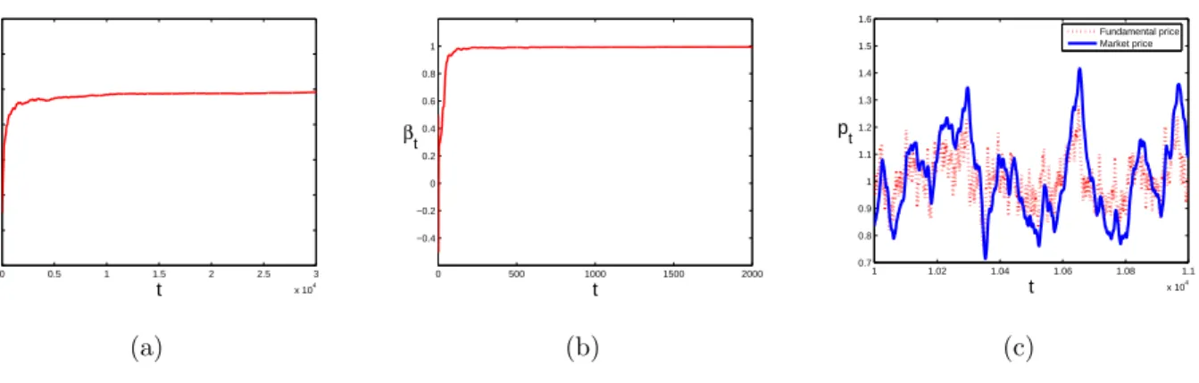
0 0.5 1 1.5 2 2.5 3 x 10⁴ 0 0.2 0.4 0.6 0.8 1 1.2 t αt (a) 0 500 1000 1500 2000 −0.4 −0.2 0 0.2 0.4 0.6 0.8 1 t βt (b) 1 1.02 1.04 1.06 1.08 1.1 x 10⁴ 0.7 0.8 0.9 1 1.1 1.2 1.3 1.4 1.5 1.6 t p t Fundamental price Market price (c)
Figure 3: (a) Time seriesαt→α∗(1.0) under SAC-learning; (b) time seriesβt →β∗(0.997)
under SAC-learning; (c) time series of market prices under SAC-learning and fundamental prices. Initial values p0 = 0.3, y0 = 0.08.
3.3.1 Numerical analysis
Figure 3 shows that SAC-learning (αt, βt) converges to the unique stable SCEE (α∗, β∗).
Figure 3a indicates that the mean of the market prices under SAC-learning αt tends to
the meanα∗ = 1 in the SCEE, while Figure 3b shows that the first-order autocorrelation
coefficient of the market prices under SAC-learning βt tends to the first-order
autocor-relation coefficient β∗ = 0.997 in the SCEE. Therefore, given the same sample path of
noise, the time series of the market prices under SAC-learning is almost the same as that in the SCEE, which can be seen by comparing Figure 3c to Figure 1c. That is, the market prices under SAC-learning fluctuate around the fundamental prices but have excess volatility and stronger autocorrelation. Therefore, the self-referential SCEE and learning offer a possible explanation of bubbles within a stationary time series framework, as suggested in Bullard et al. (2010).
4
The New Keynesian Philips curve with AR(1)
driv-ing variable
Now consider a second application of SCEE and learning in macroeconomics, the New Keynesian Philips curve with an AR(1) driving variable as suggested by Lansing (2009). Assume that the inflation and the output gap (real marginal cost) evolve according to
πt =λπet+1+γyt+ut, yt =a+ρyt−1+εt, (4.1)
where πt is the inflation at time t, πte+1 is expected inflation at date t+ 1 and yt is the
output gap or real marginal cost. λ ∈[0,1) is the representative agent’s subjective time discount factor, γ > 0 is related to the degree of price stickiness in the economy and
ρ ∈ [0,1) describes the linear dependence of the output gap on its past value. ut and
εt are i.i.d. stochastic disturbances with zero mean and finite absolute moments with
variances σ2
u and σε2, respectively. The key difference with the standard asset pricing
model is that this model includes two stochastic disturbances, not only the noise εt of
the AR(1) driving variable, but also an additional noiseut in the New Keynesian Philips
curve. We refer to ut as a markup shock that is often motivated by the presence of a
variable tax rate and toεtas a demand shock that is uncorrelated with the markup shock.
4.1
Rational expectations equilibrium
If agents are rational, then a straightforward computation (see Appendix F) gives the rational expectations equilibrium
π∗ t = γλa (1−λ)(1−λρ) + γ 1−λρyt+ut. (4.2)
Hence the mean and variance of rational expectations equilibrium π∗
t are, respectively, π∗ :=E(π∗ t) = γa (1−λ)(1−ρ), (4.3) V ar(π∗t) = E(π∗t −π∗)2 = γ2σ2ε (1−λρ)2(1−ρ2)+σ 2 u. (4.4)
Furthermore, the first-order autocovariance and autocorrelation of rational expectations equilibrium π∗ t are, respectively, E(π∗ t −π∗)(π∗t−1−π∗) = γ2ρσ2 ε (1−λρ)2(1−ρ2), Corr(π∗ t, πt∗−1) = ργ2 γ2+ (1−λρ)2(1−ρ2)σu2 σ2 ε .
Note that in the special case σ2
u = 0, the above expression reduces to Corr(πt∗, π∗t−1) =ρ
as in Eq. (3.7). Moreover, the larger the noise level σ2
u in the markup shock, the smaller
4.2
Existence of first-order SCEE
Suppose now that agents are boundedly rational and that their perceived law of motion for inflation is a univariate AR(1) process.
πt=α+β(πt−1−α) +vt (4.5)
The implied actual law of motion then becomes πt=λ[α+β2(πt−1−α)] +γyt+ut, yt=a+ρyt−1+εt. (4.6) Denote the unconditional expectation of πtby ¯π and the unconditional expectation of
yt by ¯y. Then ¯y=a/(1−ρ) and ¯π satisfies
¯ π=λα(1−β2) +λβ2π¯+γy.¯ Hence ¯ π = λα(1−β 2) +γy¯ 1−λβ2 . (4.7)
Imposing the first consistency requirement on the mean, i.e. ¯π = λα(1−1−βλβ2)+2 γy¯ =α, we get
α= γy¯ 1−λ =
γa
(1−λ)(1−ρ) =:α
∗.
Therefore using (4.3), in a SCEE the unconditional mean of inflation coincides with the REE fundamental inflation.
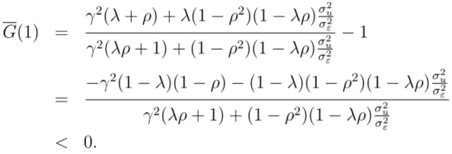
After straightforward computations (see Appendix G), we obtain
Corr(πt, πt−1) = γ2(λβ2+ρ) +λβ2(1−ρ2)(1−λβ2ρ)σu2 σ2 ε γ2(λβ2ρ+ 1) + (1−ρ2)(1−λβ2ρ)σ2u σ2 ε =:F(β). (4.8) Note that if we replace λ by 1
R, γ by
ρ
R and σu by 0, then the autocorrelation in (4.8) is
simplified to βρβ2+2+RρR, which coincides with the autocorrelation in the asset pricing model in (3.13).
The second consistency requirement of first-order autocorrelation coefficient β yields,
F(β) =β.
DefineG(β) :=F(β)−β. Since 0 < ρ <1 and 0≤λ <1,
G(0) = γ2ρ
γ2+ (1−ρ2)σu2
σ2
ε >0
and G(1) = γ 2(λ+ρ) +λ(1−ρ2)(1−λρ)σ2 u σ2 ε γ2(λρ+ 1) + (1−ρ2)(1−λρ)σ2u σ2 ε −1 = −γ 2(1−λ)(1−ρ)−(1−λ)(1−ρ2)(1−λρ)σ2 u σ2 ε γ2(λρ+ 1) + (1−ρ2)(1−λρ)σ2u σ2 ε < 0.
Therefore, there exists at least one β∗ ∈(0,1), such that G(β∗) = 0, i.e. F(β∗) = β∗. In
the special case without autocorrelation in the driving variable yt, i.e. ρ = 0, equation
(4.8) gives F(β) = λβ2. Hence the first-order SCEE for ρ = 0 is β∗ = 0 and coincides
with the REE.
Proposition 3 In the case that 0 < ρ < 1 and 0 ≤ λ < 1, there exists at least one nonzero first-order stochastic consistent expectations equilibrium (SCEE) (α∗, β∗) for the
New Keynesian Philips curve (4.6) with α∗ = γa
(1−λ)(1−ρ) =π∗.
It turns out that in the NKPC multiple SCEE may co-exist. To see this, rewrite the first-order autocorrelation,F(β) = λβ2+ ρ(1−λ2β4)
(λβ2ρ+1)+(1−ρ2)(1−λβ2ρ)1
γ2·
σ2u σε2
. It is easy to see that if γ or σ2ε
σ2
u increases, then F(β) increases, and therefore multiple SCEE may occur. The
simulations in the following subsection illustrate this point more clearly.
4.2.1 Numerical analysis
Now we illustrate the existence of SCEE and the effects of ρ, γ and σε2
σ2
u numerically.
Based on empirical findings, such as Lansing (2009), Gali et al. (2001) and Fuhrer (2006, 2009), we first examine a plausible case8in whichγ = 0.075, σ
u = 0.003162, σε = 0.01, ρ= 0.9, λ = 0.99, εt ∼ N(0, σε2), ut ∼ N(0, σu2), a = 0.0004. Hence σ 2 u σ2 ε = 0.1. Figure 4a
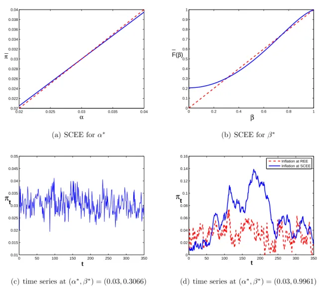
illustrates existence of a unique (stable) α∗, where α∗ = 0.03. Figure 4b shows that
there exist three β∗, where β∗ = 0.3066,0.7417,0.9961. That is, there exist three
first-order SCEE: two stable ones (α∗, β∗) = (0.03,0.3066),(0.03,0.9961) and an unstable
8As shown in Lansing (2009), based on regressions using either the output gap or labor’s share of
income over the period 1949.Q1 to 2004.Q4, ρ = 0.9, σε = 0.01. Estimates of the NKPC parameters
λ, γ, σuare sensitive to the choice of the driving variable, the sample period, and the econometric model etc. Later we also examine the effects of some other parameters on SCEE. Furthermore, based on the above theoretical results, a just affects the mean of inflation ¯π but not the autocorrelation coefficient
one (α∗, β∗) = (0.03,0.7417). Considering that the SAC-learning converges to a stable
SCEE (see the next subsection), the stable (learnable) SCEE are the most interesting. Figures 4c and 4d illustrate the two time series for the two (stable) SCEE (α∗, β∗) =
(0.03,0.3066),(0.03,0.9961), suggesting that inflation has different persistence at different SCEE. That is, the SCEE is an important factor in affecting inflation persistence. In fact, the time series of inflation in the SCEE with high β∗ in Figure 4d has similar
persistence characteristics and amplitude of fluctuation as in empirical inflation data in Tallman (2003). Furthermore, Figure 4d illustrates that inflation in the SCEE with high
β∗ has stronger persistence than the REE inflation, where the first-order autocorrelation
coefficient of REE inflation is 0.865 less thanβ∗ = 0.9961.
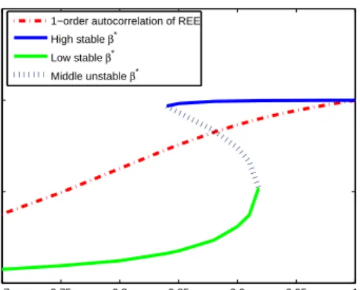
In order to further study the effects of ρ, Figure 5 illustrates SCEE β∗ together
with the first-order autocorrelation coefficient of REE inflation as functions of ρ. For 0.84 < ρ < 0.918, two stable SCEE β∗ exist separated by an unstable SCEE. The large
SCEE β∗ is larger than the first-order autocorrelation coefficient of REE inflation, while
the small SCEE β∗ is smaller than the first-order autocorrelation coefficient of REE
in-flation. In the next subsection we will show that for a large range of initial values of inflation the SAC-learning converges to the stable high SCEEβ∗ with strong persistence.
If ρ > 0.918, there exists only one stable SCEE β∗ with stronger persistence than REE.
Therefore for plausible values of ρ around 0.9, inflation in a SCEE often generates high-persistence as shown in Figure 4d. This result is consistent with the empirical finding in Adam (2007) that the Restricted Receptions Equilibrium (RPE) describes subjects’ inflation expectations surprisingly well and provides a better explanation for the observed persistence of inflation than REE.
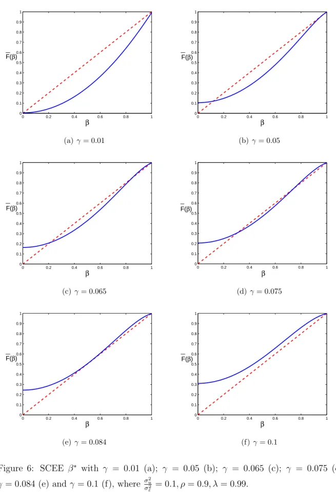
Figure 6 illustrates how the number of SCEE depends onγ. The simulations show that for plausibleγ there exist at least one and at most three SCEE β∗. For sufficiently small
γ(<0.05), there exists only one lowβ∗, as shown in Figure 6a. As γ increases, the graph
ofF(β) = λβ2+ ρ(1−λ2β4) (λβ2ρ+1)+(1−ρ2)(1−λβ2ρ) 1
γ2· σu2 σ2ε
goes up. Atγ = 0.05, a new SCEEβ∗ ≈0.975
is created at a tangent bifurcation, see Figure 6b. Immediately after that there exist three
β∗, two stable equilibria and one unstable. That is, at γ = 0.05, a tangent bifurcation
occurs. Figures 6c and 6d illustrate the three β∗ with the high stable β∗ close to 1. As
γ increases, the two stable β∗-values grow. At γ = 0.084, another tangent bifurcation
occurs, where the lowerβ∗-values coincide, as shown in Figure 6e. Forγ >0.084, there is
0.02 0.025 0.03 0.035 0.04 0.02 0.022 0.024 0.026 0.028 0.03 0.032 0.034 0.036 0.038 0.04 α π
(a) SCEE forα∗
0 0.2 0.4 0.6 0.8 1 0 0.1 0.2 0.3 0.4 0.5 0.6 0.7 0.8 0.9 1 β F(β) (b) SCEE forβ∗ 0 50 100 150 200 250 300 350 0.01 0.015 0.02 0.025 0.03 0.035 0.04 0.045 0.05 t πt (c) time series at (α∗, β∗) = (0.03,0.3066) 0 50 100 150 200 250 300 350 0 0.02 0.04 0.06 0.08 0.1 0.12 0.14 0.16 t πt Inflation at REE Inflation at SCEE (d) time series at (α∗, β∗) = (0.03,0.9961)
Figure 4: (a) SCEE α∗ is the unique intersection point of the mean of inflation ¯π =
λα(1−β2)+γy¯
1−λβ2 (bold curve) with the perceived mean α (dotted line); (b) SCEE β∗ is an intersection point of the first-order autocorrelation of inflation γ
2(λβ2+ρ)+λβ2(1−ρ2)(1−λβ2ρ)σ2u σ2ε
γ2(λβ2ρ+1)+(1−ρ2)(1−λβ2ρ)σ2u σ2ε
(bold curve) and the perceived first-order autocorrelation β (dotted line); (c) time series of inflation in stable low-persistence SCEE (α∗, β∗) = (0.03,0.3066); (d) times series of
inflation in stable high-persistence SCEE (α∗, β∗) = (0.03,0.9961) (bold curve) and time
series of REE inflation (dotted curve), where γ = 0.075, σu = 0.003162, σε = 0.01, ρ =
0.7 0.75 0.8 0.85 0.9 0.95 1 0 0.5 1 1.5 ρ β*
1−order autocorrelation of REE High stable β*
Low stable β* Middle unstable β*
Figure 5: First-order autocorrelation coefficient of REE inflation (dotted real curve), stable SCEEβ∗ with respect toρ(bold curves), unstable SCEE β∗ (dotted curve), where
γ = 0.075, σu = 0.003162, σε = 0.01, λ= 0.99.
Hence a larger γ tends to lead to higher persistence of inflation. Intuitively with a larger
γ, it can be seen from (4.1) that the driving variable (output gap or real marginal cost) has a larger impact on inflation. Hence when the driving variable is relatively important, a high-persistence SCEE occurs. If on the other hand, σ2
u increases, that is, the noise
to inflation increases, the ratio σ2ε
σ2
u decreases and the strong reverses and low-persistence
SCEE become more likely. That is, intuitively clear, as more noise to inflation dominates the driving variable, this leads to a low-persistence inflation equilibrium.
4.3
Stability under SAC-learning
The SAC-learning dynamics in the New Keynesian Philips curve with AR(1) driving variable is given by πt =λ[αt−1+βt2−1(πt−1−αt−1)] +γyt+ut, yt =a+ρyt−1+εt. (4.9) with αt, βt as in (2.8). This is another expectations feedback system with expectation
feedback from inflation forecasting. Realized inflations influence the beliefs agents have about economic reality and these beliefs feed back into the actual dynamics of economy and determine the future realized inflations together with an exogenous driving variable output gap or real marginal costs.
We further check the relationship between stability of SCEE (α∗, β∗) and SAC-learning.
Forα∗, since 0 ≤ λ(1−β2)
0 0.2 0.4 0.6 0.8 1 0 0.1 0.2 0.3 0.4 0.5 0.6 0.7 0.8 0.9 1 β F(β) (a) γ= 0.01 0 0.2 0.4 0.6 0.8 1 0 0.1 0.2 0.3 0.4 0.5 0.6 0.7 0.8 0.9 1 β F(β) (b) γ= 0.05 0 0.2 0.4 0.6 0.8 1 0 0.1 0.2 0.3 0.4 0.5 0.6 0.7 0.8 0.9 1 β F(β) (c) γ= 0.065 0 0.2 0.4 0.6 0.8 1 0 0.1 0.2 0.3 0.4 0.5 0.6 0.7 0.8 0.9 1 β F(β) (d)γ= 0.075 0 0.2 0.4 0.6 0.8 1 0 0.1 0.2 0.3 0.4 0.5 0.6 0.7 0.8 0.9 1 β F(β) (e) γ= 0.084 0 0.2 0.4 0.6 0.8 1 0 0.1 0.2 0.3 0.4 0.5 0.6 0.7 0.8 0.9 1 β F(β) (f) γ= 0.1
Figure 6: SCEE β∗ with γ = 0.01 (a); γ = 0.05 (b); γ = 0.065 (c); γ = 0.075 (d);
γ = 0.084 (e) and γ = 0.1 (f), where σ2u
σ2
of the complexity of the first-order autocorrelation F(β) in (4.8), it is difficult to check the stability of SCEE, or even the number of SCEE. We have the following relationship between the SCEE and the SAC-learning.
Proposition 4 If (0≤)F0(β∗) < 1, then the SCEE (α∗, β∗) is stable, that is, the
SAC-learning (αt, βt) converges to the SCEE (α∗, β∗) as time t tends to ∞.
The proof is given in Appendix H. If the stable SCEE is not unique, the convergence de-pends on initial states of the system, as illustrated in the following numerical simulations.
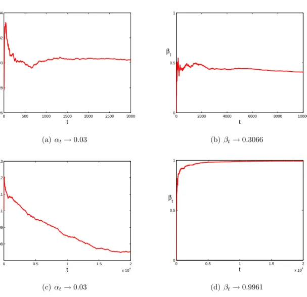
4.3.1 Numerical analysis
For (π0, y0) = (0.028,0.01), Figures 7a and 7b show that the SAC-learning dynamics
(αt, βt) converges to the stable low-persistence SCEE (α∗, β∗) = (0.03,0.3066). Figure
7a illustrates that the mean of inflation αt tends to the mean α∗ = 0.03. Figure 7b
illustrates that the first-order autocorrelation coefficient of inflation βt slowly tends to
the low-persistence stable first-order autocorrelation coefficient β∗ = 0.3066. For the
different initial value (π0, y0) = (0.1,0.15), our numerical simulation shows that the mean
of inflation αt under SAC-learning still tends to the mean α∗, but slowly9 (see Figure
7c), while Figure 7d indicates that the first-order autocorrelation coefficient of inflation
βt under SAC-learning tends to the higher stable first-order autocorrelation coefficient
β∗ = 0.996110. Correspondingly given the same sample path of noise, the time series of
inflation under SAC-learning can also replicate the time series of inflation in the SCEE after long-term learning as shown in the preceding asset pricing model.
Numerous simulations show that as initial values of inflation are (relatively) higher than the mean α∗ = 0.03, the sample autocorrelation learning β
t generally enters the
high-persistence region. In particular, a large shock to the inflation may easily cause a jump of the SAC-learning process into the high-persistence region.
5
Conclusion
In this paper we have introduced the concept of behavioral learning equilibrium, a very simple type of misspecification equilibrium together with an intuitive behavioral
9The slow convergence is caused by the slope λ−λβ2
1−λβ2 in the expression (4.7), which is very close to 1
forλ= 0.99, as shown in Figure 4a.
0 500 1000 1500 2000 2500 3000 0.026 0.028 0.03 0.032 0.034 t αt (a) αt→0.03 0 2000 4000 6000 8000 10000 0 0.5 1 t βt (b)βt→0.3066 0 0.5 1 1.5 2 x 10⁴ 0.08 0.09 0.1 0.11 0.12 0.13 t αt (c) αt→0.03 0 0.5 1 1.5 2 x 10⁴ 0 0.5 1 t βt (d)βt→0.9961
Figure 7: Time series of αt and βt under SAC-learning with different initial values
learning process. Boundedly rational agents use a univariate linear forecasting rule and in equilibrium correctly forecast the unconditional sample mean and first-order sample autocorrelation. Hence, to a first order approximation the simple linear forecasting rule is consistent with observed market realizations. Sample autocorrelation learning simply means that agents are slowly updating the two coefficients –sample mean and first-order autocorrelation– of their linear rule. In the long run, agents thus learn the best univariate linear forecasting rule, without fully recognizing the structure of the economy.
We have applied our behavioral learning equilibrium concept to a standard asset pric-ing model with AR(1) dividends and a New Keynesian Philips curve driven by an AR(1) process for the output gap or marginal costs. In both applications, the law of motion of the economy is linear, but it is driven by an exogenous stochastic AR(1) process. Agents however are not fully aware of the exact linear structure of the economy, but use a simple univariate forecasting rule, to predict asset prices or inflation. In the asset pricing model a unique SCEE exists and it is globally stable under SAC-learning. An important fea-ture of the SCEE is that it is characterized by high-persistence and excess volatility in asset prices, significantly higher than under rational expectations. In the New Keynesian model, multiple SCEE arise and a low and a high-persistence misspecification equilib-rium co-exist. The SAC-learning exhibits path dependence and it depends on the initial states whether the system converges to the low-persistence or the high-persistence infla-tion regime. In particular, when there are shocks– e.g. oil shocks– temporarily causing high inflation, SAC-learning may lock into the high-persistence inflation regime.
Are these behavioral learning equilibria empirically relevant or would smart agents recognize their (second order) mistakes and learn to be perfectly rational? This empirical question should be addressed in more detail in future work, but we provide some argu-ments for the empirical relevance of our equilibrium concept. Firstly, in our applications the SCEE already explain some important stylized facts: (i) high persistence (close to unit root) and excess volatility in asset prices, (ii) high persistence in inflation and (iii) regime switching in inflation dynamics, which could explain a long phase of high US in-flation in the 1970s and early 1980s as well as a long phase of low inin-flation in the 1990s and 2000s. Secondly, we stress the simplicity andbehavioralinterpretation of our learning equilibrium concept. The univariate AR(1) rule and the SAC-learning process are exam-ples of simple forecasting heuristics that can be used without any knowledge of statistical techniques, simply by observing a time series and roughly ”guestimating” its sample av-erage and its first-order persistence coefficient. Coordination on a behavioral forecasting
heuristic that performs reasonably well to a first-order approximation seems more likely than coordination on more complicated learning or sunspot equilibria, cf., for example, Woodford (1990). Even though some smart individual agents might be able to improve upon the best linear, univariate forecasting rule, a majority of agents might still stick to their simple univariate rule. It therefore seems relevant to describe aggregate phenomena by simple misspecification equilibria and behavioral learning processes. Our behavioral learning equilibrium concept also relates to the “natural expectations” in Fuster et al. (2010), emphasizing parsimonious forecasting rules giving much weight to recent changes to explain the long-run persistence of economic shocks. Our simple univariate AR(1) rule may be seen as the most parsimonious forecasting rule leading to long-run persistence. There is in fact already some experimental evidence for the relevance of misspecification equilibria in Adam (2007). More recently Assenza et al. (2011) and Pfajfar and Zakelj (2010) ran learning to forecasting experiments with human subjects in a New Keynesian framework with expectations feedback from individual inflation and output gap forecasts. Simple linear univariate models explain a substantial part of individual inflation and output gap forecasting behavior.
In future work we plan to consider more general economic settings and study behav-ioral learning equilibria. An obvious next step is to apply our SCEE and SAC-learning framework to higher dimensional linear economic systems, with agents forecasting by uni-variate linear rules. In particular, the fully specified New Keynesian model of inflation and output dynamics would be an interesting (two-dimensional) application. Finally, it is interesting and challenging to study SCEE and misspecification under heterogeneous expectations and allow for switching between different rules. Branch (2004) and Hommes (2011) provide some empirical and experimental evidence on heterogeneous expectations, while Berardi (2007) and Branch and Evans (2006, 2007) have made some related studies on heterogeneous expectations and learning in similar settings.
Acknowledgements
We would like to thank Kevin Lansing, Mikhail Anufriev, Michael Reiter, Florian Wagener, Cees Diks and other participants in the KAFEE lunch seminar at the University of Amsterdam, March 2011, the 3rd POLHIA workshop in Universita Politecnica delle Marche, Ancona, May 2010, the 11th Workshop on Optimal Control, Dynamic Games and Nonlinear Dynamics at the University of Amsterdam, June 2010 and the CEF 2011