Metric Learning for Automatic Sleep Stage Classification

Kent Academic Repository

Full text document (pdf)

Copyright & reuse

Content in the Kent Academic Repository is made available for research purposes. Unless otherwise stated all content is protected by copyright and in the absence of an open licence (eg Creative Commons), permissions for further reuse of content should be sought from the publisher, author or other copyright holder.

Versions of research

The version in the Kent Academic Repository may differ from the final published version.

Users are advised to check http://kar.kent.ac.uk for the status of the paper. Users should always cite the published version of record.

Enquiries

For any further enquiries regarding the licence status of this document, please contact: [email protected]

If you believe this document infringes copyright then please contact the KAR admin team with the take-down information provided at http://kar.kent.ac.uk/contact.html

Citation for published version

Phan, Huy and Do, Quan and Do, The-Luan and Vu, Duc-Lung (2013) Metric Learning for Automatic

Sleep Stage Classification. In: 35th Annual International Conference of the IEEE Engineering

in Medicine and Biology Society (EMBC 2013). IEEE pp. 5025-5028.

DOI

https://doi.org/10.1109/EMBC.2013.6610677

Link to record in KAR

https://kar.kent.ac.uk/72696/

Document Version

Metric Learning for Automatic Sleep Stage Classification

Huy Phan

, Quan Do

, The-Luan Do

, and Duc-Lung Vu

Abstract— We introduce in this paper a metric learning approach for automatic sleep stage classification based on single-channel EEG data. We show that learning a global metric from training data instead of using the default Euclidean metric, thek-nearest neighbor classification rule outperforms state-of-the-art methods on Sleep-EDF dataset with various classification settings. The overall accuracy for Awake/Sleep and 4-class classification setting are 98.32 % and 94.49 % respectively. Furthermore, the superior accuracy is achieved by performing classification on a low-dimensional feature space derived from time and frequency domains and without the need for artifact removal as a preprocessing step.

I. INTRODUCTION

The study of sleep is highly important in health care since sleep disorders affect the well-being and productivity of many individuals. The foundation of sleep classification was first laid in 1953 [7], since then has remained an important research topic. Sleep scoring based on polysomnography can be visually performed by a human expert to classify every 30-second epochs of EEG data into different sleep stages, following Rechtschaffen and Kales (R&K) rules [6] and based on the structure of the signal. However, it is a very time-consuming and labor-intensive task.

During the last decades, different approaches for automatic sleep stage classification using EEG signal have been pro-posed. Most of them are similar in the way that features characterizing each EEG data epoch will be first extracted, followed by a classification algorithm to assign class label to each data epoch. Feature extraction usually relies on time-domain analysis [14], spectral analysis [13], wavelet decom-position [8] [12], and even unsupervised feature learning [15]. Typical classification algorithms are neural networks [8], hidden makov models [9], k-means clustering [10], k -nearest neighbors (kNN) [11], support vector machines [12] to name a few. Comparative study on performance of these classifiers has also been conducted in [11]. Sleep stage classification based EEG data also involves in using single-channel EEG signal [8], multi-single-channel EEG signals [12] [13], and multimodal combination with other signals such as EOG, EMG and ECG signals [12].

In this paper, we re-visit the fundamental issue of machine learning: how to measure dissimilarity/similarity between samples. Without prior knowledge, Euclidean distance is implicitly employed in most proposed classifiers to measure the dissimilarities between examples represented as vector

1,2,3,4

H. Phan, Q. Do, T. L. Do, and D. L. Vu are with Department of Computer Engineering, University of Information Technology, Km 20, Ha Noi highway, Linh Trung ward, Thu Duc district, HCMC, Viet-nam huypq at uit.edu.vn, quando at uit.edu.vn, luandt at uit.edu.vn, lungvd at uit.edu.vn

inputs. Although the Euclidean distance is convenient and intuitive, it ignores the fact that the semantic meaning of “similarity” is inherently task- and data-dependent [1]. Ide-ally, the distance metric should be adapted to the particular problem. Inspired by this, we show in this paper learning a global distance metric from labeled examples and using it in kNN classification significantly improve performance for sleep staging although only a few features extracted from single-channel EEG data. We also study the effects of dimensionality reduction, which is implicit during learning distance metric, on the classification accuracy.

II. EEG SIGNAL, SLEEP STAGES, AND SLEEP EEG DATASET

A. EEG Signal

Based on electrical recordings taken on the scalp of a sub-ject, the Electroencephalogram (EEG) signal measurements are able to provide information about activities of the brain. It is the most important signal in sleep stage classification no matter manual scoring by human experts or automatic classification systems. Analyzing the information obtained from the EEG measurements can help carry out inference and studies about sleep.

B. Sleep Stages

According to R&K sleep scoring standard [6], sleep are divided into two major stages named rapid eye movement (REM) and non-rapid eye movement (NREM). Further, NREM is divided into four sub-stages: 1, 2, 3, and 4, making up to totally 6 sleep stages (including awake).

Stage 1, usually lasting between 1-5 minutes and con-tributing 4-5% of total sleep, is a transition stage between wakefulness and sleep. It consists of a low-voltage EEG tracing with well-defined alpha and theta activity, occasional vertex spikes, and slow rolling eye movements (SEMs) [8].

Stage 2 is considered as the “baseline” of sleep and comprises 45-55% of complete sleep duration. It is char-acterized by a relatively low-voltage, mixed-frequency EEG background burried in the occurrence of sleep spindles [16] and K-complexes [17]. Alternatively, high-voltage delta waves may appear up to 20% of Stage 2.

Stage 3constitutes 4-6% of total sleep duration and usually only appears in the first one-third of the sleep episode. During at least 20% and at most 50% of this stage, EEG signals exhibit strongly discriminative characteristics with

≤2Hz frequencies and ≥75V amplitudes (delta waves).

Stage 4 contributes 12-15% to the total sleep duration. Characteristics of Stages 3 and 4 are quite similar and they are known as slow wave sleep (SWS). The difference is that, during Stage 4, delta waves cover≥50% of the record.

REM, in which dreaming occurs, is characterized by rapid eye movements under closed eyelids, motor atonia, and low voltage EEG patterns. REM constitutes 20-25% of a normal sleep night. During REM sleep, the brain activity is reversed from Stage 4 to a pattern similar to Stage 1 [8].

C. Sleep EEG Dataset

The experiments presented in this paper are based on the Sleep-EDF database [3] obtained from the PhysioBank online resource. We only used four recordings: sc4002e0, sc4012e0, sc4102e0, and sc4112e0 which were recorded in 1989 over the course of one full day from healthy male and female pioneers between 21 and 35 years old. These recordings include horizontal electrooculogram (EOG), Fpz-Cz and Pz-O channels of EEG, submental-electromyogram (EMG) envelope, oronasal airflow, and rectal body temper-ature. Since we aimed at illustrating efficiency of learning a metric for sleep staging with single EEG channel, we only use Fpz-Oz EEG sampled at 100 Hz for analysis. The hypnogram data accompanying with the dataset was used as ground truth to evaluate performance of the classification algorithm in the experiments. It was created by manual scoring according to R&K using the two EEG channels.

III. SLEEP STAGE CLASSIFICATION MODEL

A. Feature Extraction

We derive the following features for each 30-second single-channel EEG data epoch.

Statistical measuresThese include variance, skewness, and kurtosis. The variance is to characterize the spread of the data while the skewness represents the asymmetry around the sample mean. The kurtosis measures how the distribution is prone to outliers.

Spindle scoreSimilar to the features used in [2], the overall spindle score presents the percentage of the signal classified as spindle activity. Spindle activity refers to segments of the EEG signal with two peaks and two troughs created by the difference between five consecutive points changes from positive to negative in straight. In order to search for these patterns at different frequencies, a lag parameter was used. This parameter indicates the width in sample points of each rise or fall. In this study, with data sampled at 100 Hz, the lag parameter was set to 5 to allow for detection of spindles in 8-12 Hz frequency range.

Permutation entropy (PE) The permutation entropy is to measure the “uncertainty’ of the EEG signal. Similar to the spindle score, it searches for patterns such as peaks, troughs, and slopes in the signal but its values depends on the distribution of these patterns. An equal distribution of all patterns will produce a maximum value while a minimum value will be induced when only a single pattern is present. Here we consider two PE measures respective to two lag parameter values of 1 and 2. As in [4], the threshold was set at 1% of the interquartile range of the data.

Power in different frequency bandsWe computed the total power in five frequency bands, including delta (up to 4 Hz), theta (4-7.5 Hz), alpha (7.5-12 Hz), beta (12-26 Hz), and gamma (above 26 Hz) [18], adding other five features.

Total power The total power in all five frequency bands was also computed as used as a feature.

Properties of log power These features present charac-teristics of the log of the power spectral density (PSD) on delta and alpha bands [5]. First, we performed linear fitting in delta (0.5-4 Hz) and alpha (8-17 Hz) frequency bands to determine the slope and offset. After that, we could extract the maximum values of the PSD above the linear estimate in the delta and alpha frequency ranges. Generally, a prominent peak will produce a large value. Two frequency values correspond to these maximum values are also extracted.

Power fractions The low and high power fractions with respect to low frequency ranges (delta and theta ranges) and high frequency ranges (beta and gamma ranges) were also computed by summing the power in the individual ranges and dividing by the total power.

By this feature extraction, each 30-second EEG data epoch is represented by a 17-dimensional vector inputs. These inputs are then used in classification algorithm. To motivate further research, the Matlab source code will be made publicly available.

B. Metric Learning with Large Margin Nearest Neighbor

Given a training data set of instances labeled with their true class labels, thekNN algorithm assigns the class label to a new data instance. The class label is obtained from the majority vote of thekclosest instances in training data. In order to measure the closeness, a distance metric needs to be pre-defined. Without prior knowledge, a Euclidean distance is implicitly employed. However, as discussed, the distance metric should be adapted to the particular problem and learned from the training data. Large Margin Nearest Neighbors (LMNN) algorithm [1] can learn this global metric in a supervised fashion to improve the classification accuracy of thekNN rule.

Let the training data consist of a data set D = (x₁, y₁), . . . ,(xn, yn)⊂ Rm× C, where the set of possible

classes isC= 1, . . . , c. LMNN learns a metric of type:

D(xi, xj) = (xi−xj)TM(xi−xj) =||L(xi−xj)||

2

(1)

The matrix M needs to be positive semi-definite for the metric D(·,·) to be well defined. In the special case of the Euclidean metric, the matrix M is identity. For generalization, the metricD(·,·)is often referred as Mahalanobis metric.

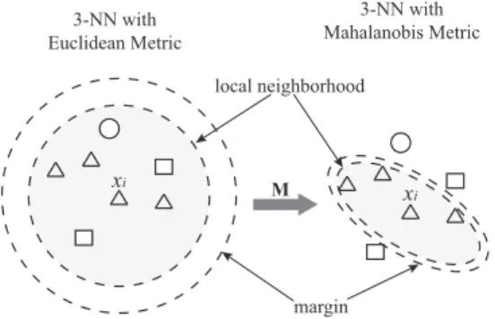
LMNN optimizes the matrix M with two objectives: minimize the distances between examples in the same class, and in the meantime keep examples from different classes far away. Fig. 1 show an example of such an optimization.

With the learned metric in Fig. 1, the input vectorx~i is

surrounded by training instances of the same class. If it was a test sample, it would be classified correctly under k = 3 nearest neighbor rule. It leads to the final optimization problem as in (2):

margin local neighborhood 3-NN with Euclidean Metric 3-NN with Mahalanobis Metric xi xi M

Fig. 1. Illustration of 3-NN algorithm with Euclidean and Mahanalobis metrics. minimize X ij ηij(xi−xj)TM(xi−xj) +CX ijl ηij(1−yil)ξijl (2) subject to          (i)(xi−xl)TM(xi−xl) −(xi−xj)TM(xi−xj)≥1−ξijl (ii)ξijl≥0 (iii)M 0

where the binary value yij indicates whether samples

xi and xj are in the same class and the binary value ηij

indicating whether xj is a selected nearby neighbor of xi

with the same class, andξijlare slack variables.

Intuitively, the first term in the objective function is to minimize the distances between all training samples and their selected neighbors. The second term is to maximize the margin between same-class distances (xitoxj) and

different-class distances (xi toxl) of all training samples. The margin

is relaxed by slack variables and is of exactly one unit fixed by the scale of the matrixM. Any alternative choiceC >0

would result in rescaling ofM by a factor of1/C. We use the implementation of this algorithm provided by the authors of [1], thanks for their efforts.

Furthermore, LMNN can be used as a supervised dimen-sionality reduction by optimizing on matrix L rather than matrixM=LT_{L and constrainL to be rectangular of size}

r×m, where r is the desired output dimensionality which is presumed to be smaller than the input dimensionality,m.

IV. EXPERIMENT

A. 4-class Classification

For Stage 1 of NREM sleep and REM sleep, EEG signals are similar and, thus, can be merged into one class. Hence, we attempt to classify four sleep stages consisting of Awake, Stage1 + REM, Stage 2 and Slow Wave Stage (SWS). In addition, this partition is consistent with the previous work in [8] using the same dataset, allow us properly comparing performance. It is also considerable to notice that we neither preprocess the data for artifact removal nor apply bootstrap-ping to lessen affects of imbalanced data as in [8].

The number of data epochs of each class in the dataset is tabulated in Table I. We randomly divide the data set into training set (70 %) and test set (30 %). The features are

TABLE I

NUMBER OF DATA EPOCHS OF4CLASSES IN THE DATASET

Wake Stage 1 + REM Stage 2 SWS

7722 1027 2036 529 1 2 3 4 5 6 7 8 9 10 11 12 13 14 15 16 17 80 81 82 83 84 85 86 87 88 89 90 91 92 93 94 95 Dimension Classification Accuracy (%)

Fig. 2. Training and testing accuracy (blue and red bars respectively) according to different dimensionality reduction settings.

extracted from 30-second segments of Pz-Oz channel. The transformation matrix is learned from the training data and the test data is used to evaluate the classification accuracy.

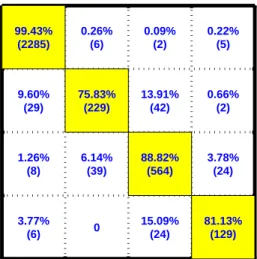
Since dimensionality of the feature space is quite small (17 dimensions), we investigate different dimensionality re-duction by settingrto be running from 1 to 17 with a step of 1. The variation of overall training and testing classification accuracy according to different dimensionality is illustrated in the Fig. 2. The highest testing accuracy, 94.49 %, is obtained at r = 8 with the learned Mahalanobis metric, compared to 91.48 % by using the default Euclidean metric. For the sake of comparison, this result outperforms not only the work using Sleep-EDF dataset with similar setting [8] with the average accuracy of 93 %, but also other works using private multi-channel recorded data such as [12] with the average accuracy of 93 %. For further detail, Fig.3 exhibits 4-class classification confusion matrix over the test set with r = 8. Out of 4 classes, “Wake” and “S1 + REM” classes are most and least discriminative with the classification accuracy of 99.43 % and 75.83 % respectively. The superior overall testing accuracy is owning to that the “Wake” class’ contributes the strongest weight due to its largest cardinality.

B. Awake/Sleep Classification

Considering Awake/sleep classification setting, similar ex-perimental study is conducted. The whole dataset, out of which the number of data epochs of “Awake” and “Sleep” classes are 7722 and 3592 respectively, is divided into training set (70 %) and test set (30 %). The features are again extracted from 30-second segments of Pz-Oz channel. The study of dimensionality reduction shows that the average testing accuracy is up to 98.32 % with r= 11. This result outperforms the classification accuracy of 95 % reported in a recent study [12] which uses their own recorded multi-channel EEG data.

C. Discussion

It is worth noting that artifact removal as having been done in [8], which removed most artifact epochs, would

99.43% (2285) 0.26% (6) 0.09% (2) 0.22% (5) 9.60% (29) 75.83% (229) 13.91% (42) 0.66% (2) 1.26% (8) 6.14% (39) 88.82% (564) 3.78% (24) 3.77% (6) 0 15.09% (24) 81.13% (129) Wake S1 + REM S2 SWS Wake S1 + REM S2 SWS

Fig. 3. 4-class classification confusion matrix respective tor= 8.

further benefit the learning process. Artifact epochs which are contaminated by eye movements, blinks, muscle, heart and line noise [19] are semi-automatically removed to refine the data. However, it would greatly degrade the automatic of the classification system since we need to visually inspect the data epochs before feeding to the system.

Other machine learning techniques may also benefit this proposed metric learning approach. As can be seen from Table I, the number of data epochs of the “Wake” class is much larger than that of the “SWS” class. Boostrapping [20] is a technique to generates more data from the original dataset to reduce the skewness of the dataset when cardinality of a class is much smaller comparing to other classes. As a result, it facilitates the learning process. Exploring other features which better represents the data is a general technique to boost the performance of a classification system. Higher feature space for sleep stage classification that has been investigated in literature work such as [14] [8] can be readily integrate into the metric learning framework. The features can be also learned from the data itself instead of feature engineering [15]. In addition, multi-channel EEG and other signals like EOG, EMG and ECG have been proved to be useful for not only visually sleep scoring [21] but also automatic sleep stage classification [18]. By learning a metric over multimodal data, we can increase accuracy and reliability of the classification system.

V. CONCLUSIONS

A metric learning approach has been proposed to ad-dress automatic sleep stage classification. By learning a Mahalanobis distance metric from labeled samples, thekNN classification rule empirically outperforms the classification accuracy reported in other literature works using similar settings. Furthermore, we do not perform any preprocessing steps such as artifact removal or boostrapping. This excellent result indicates the potential of metric learning in addressing biomedical signal processing problems.

REFERENCES

[1] K. Q. Weinberger and L. K. Saul, “Distance metric learning for large margin nearest neighbor classification”. J. of Machine Learning Research, vol. 10, pp. 207-244, Jan. 2009.

[2] E. C. McKay, J. W. Sleigh, L. J. Voss, and J. P. Barnard, “Episodic waveforms in the electroencephalogram during general anaesthesia: A study of patterns of response to noxious stimuli”. Anaesthesia and Intensive Care, vol. 38, no. 1, pp. 102-112, Jan 2010.

[3] B. Kemp, “The Sleep-EDF Database”.

http://www.physionet.org/physiobank/database/sleep-edf/. Accessed January 2012.

[4] E. Olofsen, J. W. Sleigh, and A. Dahan, “Permutation entropy of the electroencephalogram: A measure of anaesthetic drug effect”. British J. of Anaesthesia, vol, 101, no. 6, pp. 810-821, 2008.

[5] K. Leslie, J. Sleigh, M. Paech, L. Voss, C. Lim, and C, Sleigh, “Dreaming and electroencephalographic changes during anesthesia maintained with propofol or desflurane”. Anesthesiology, vol. 111, no. 3, pp. 547-555, 2009.

[6] A. Rechtschaffen and A. Kales, “A Manual of Standardized Termi-nology, Technique and Scoring System for Sleep Stages of Human Subjects”. Public Health Service, U.S, Government Printing Office, Washington, DC, 1968.

[7] E. Aserinsky and N. Kleitman, “Regularly occurring periods of eye motility, and concomitant phenomena during sleep”. Science, vol. 118, pp. 273-274, 1953.

[8] F. Ebrahimi, M. Mikaeili, E. Estrada, and H. Nazeran, “Automatic Sleep Stage Classification Based on EEG Signals by Using Neural Networks and Wavelet Packet Coefficients,” Proc. IEEE EMBS’08, pp. 1151-1154, 2008.

[9] L. Doroshenkov, V. Konyshev, S. Selishchev, “Classification of human sleep stages based on EEG processing using hidden markov models”. Biomedical Engineering, vol.41, no. 1, pp. 25-28, 2007.

[10] S. Gunes, K. Polat, and S. Yosunkaya, “Efficient sleep stage recog-nition system based on EEG signal using k-means clustering based feature weighting”. Expert Systems with Applications, vol.37, no. 12, 2010.

[11] G. Becq, S. Charbonnier, F. Chapotot, A. Buguet, L. Bourdon, and P. Baconnier, “Comparison between five classifiers for automatic scoring of human sleep recordings,” In: S.K. Halgamuge, L. Wang (Eds.), Studies in Computational Intelligence (SCI), vol.4: Classification and Clustering for Knowledge Discovery, Springer-Verlag, pp. 113-127, 2005.

[12] S. Khalighi, T. Sousa, D. Oliveira, G. Pires, and U. Nunes, “Efficient feature selection for sleep staging based on maximal overlap discrete wavelet transform and SVM,” Proc. in EBMC’11, pp. 3306-3309, 2011.

[13] Y. Li, K.M. Wong, and H. de Bruin, “Electroencephalogram signals classification for sleep state decision a Riemannian geometry ap-proach”. IET Signal Processing, vol. 6, no. 4, pp. 288-299, 2012. [14] C. Vural and M. Yildiz, “Determination of Sleep Stage Separation

Ability of Features Extracted from EEG Signals Using Principle Component Analysis”. J. of Medical Systems, vol. 34, no. 1, pp. 83-89, 2010.

[15] M. Langkvist, L. Karlsson, and A. Loutfi, “Sleep Stage Classification Using Unsupervised Feature Learning”. Advances in Artificial Neural Systems, doi:10.1155/2012/107046, 2012.

[16] L. De Gennaro and M. Ferrara, “Sleep spindles: an overview”. Sleep medicine reviews, vol. 7, no. 5, pp. 423-440, 2003.

[17] A. L. Loomis, E. N. Harvey, and G. A. Hobart, “Cerebral states during sleep as studies by human brain potentials”. J. of Experimental Psychology, vol. 21, no. 2, pp. 127-144, 1937.

[18] B. A. Lopour, S. Tasoglu, H. E. Kirsch, J. W. Sleigh, and A. J. Szeri, “A continuous mapping of sleep states through association of EEG with a mesoscale cortical model”. J. of Computational Neuroscience, vol. 30, no. 2, pp. 471-487, 2011.

[19] T-P. Jung, S. Makeig, C. Humphries, T. W. Lee, M. J. McKeown, V. Iragui, and T. J. Sejnowski, “Removing Electroencephalographic Artifacts by Blind Source Separation,” Psychophysiology, vol. 37, pp. 163-178, 2000.

[20] Y. Hamamoto, “A bootstrap technique for nearest neighbor classifier design”. IEEE Transactions on Pattern Analysis and Machine Intelli-gence, vol. 19, no. 1, pp. 73-79, 1997.

[21] J. Shepard, Jr. M.D, “Atlas of Sleep Medicine”. Futura Publishing Company, 1991.