Fault Classification and Location Identification on Electrical Transmission Network Based on Machine Learning Methods

(1)

Virginia Commonwealth University Virginia Commonwealth University

VCU Scholars Compass

Theses and Dissertations Graduate School

2018

Fault Classification and Location Identification on Electrical

Transmission Network Based on Machine Learning Methods

Vidya Venkatesh

Follow this and additional works at: https://scholarscompass.vcu.edu/etd

Part of the Other Engineering Commons, and the Power and Energy Commons

Downloaded from Downloaded from

https://scholarscompass.vcu.edu/etd/5582

This Thesis is brought to you for free and open access by the Graduate School at VCU Scholars Compass. It has been accepted for inclusion in Theses and Dissertations by an authorized administrator of VCU Scholars Compass.

(2)

Fault Classification and Location

Identification on Electrical Transmission

Network Based on Machine Learning

Methods

A thesis submitted in partial fulfillment of the requirements for the degree of Master of Science

at Virginia Commonwealth University.

by Vidya Venkatesh

Master of Science, Electrical and Computer Engineering

Director: Dr. Umit Ozgur, Professor and Graduate Program Director, Department of Electrical and Computer Engineering

Virginia Commonwealth University Richmond, Virginia

(3)

Copyright Page

(4)

Acknowledgements

I would like to express my gratitude to those who helped me throughout completion of this work. First, I would like to thank my advisor, Dr. Carl Elks, for giving me the opportunity to work at

VCU’s Cyber Physical Systems Lab and for his expert advice and encouragement throughout the past two years.

This work would not have been possible without the support of Dominion Energy, VA. I am especially indebted to Brian Starling, whose constant encouragement and support throughout has made this research work possible. Special thanks to Jeremy Crider for his great support and willingness to help me. It has been wonderful working with you both.

Above all, I would like to thank my parents; whose love and guidance are with me in whatever I pursue. I would also thank my loving and supportive husband, Adarsh, for his constant devotion to my success and happiness. I dedicate this to my parents and Adarsh.

(5)

Abstract

FAULT CLASSIFICATION AND LOCATION IDENTIFICATION ON ELECTRICAL TRANSMISSION NETWORK BASED ON MACHINE LEARNING METHODS By: Vidya Venkatesh, MS.

A thesis submitted in partial fulfillment of the requirements for the degree of Master of Science at Virginia Commonwealth University.

Virginia Commonwealth University, 2018

Major Director: Dr. Umit Ozgur, Professor and Graduate Program Director, Department of Electrical and Computer Engineering

Power transmission network is the most important link in the country’s energy system as they carry large amounts of power at high voltages from generators to substations. Modern power system is a complex network and requires high-speed, precise, and reliable protective system. Faults in power system are unavoidable and overhead transmission line faults are generally higher compare to other major components. They not only affect the reliability of the system but also cause widespread impact on the end users. Additionally, the complexity of protecting transmission line configurations increases with as the configurations get more complex. Therefore, prediction of faults (type and location) with high accuracy increases the operational stability and reliability of the power system and helps to avoid huge power failure. Furthermore, proper operation of the protective relays requires the correct determination of the fault type as quickly as possible (e.g., reclosing relays).

With advent of smart grid, digital technology is implemented allowing deployment of sensors along the transmission lines which can collect live fault data as they contain useful information which can be used for analyzing disturbances that occur in transmission lines. In this thesis, application of machine learning algorithms for fault classification and location identification on the transmission line has been explored. They have ability to “learn” from the

data without explicitly programmed and can independently adapt when exposed to new data. The work presented makes following contributions:

(6)

1) Two different architectures are proposed which adapts to any N-terminal in the transmission line.

2) The models proposed do not require large dataset or high sampling frequency. Additionally, they can be trained quickly and generalize well to the problem.

3) The first architecture is based off decision trees for its simplicity, easy visualization which have not been used earlier. Fault location method uses traveling wave-based approach for location of faults. The method is tested with performance better than expected accuracy and fault location error is less than ±1%.

4) The second architecture uses single support vector machine to classify ten types of shunt faults and Regression model for fault location which eliminates manual work. The architecture was tested on real data and has proven to be better than first architecture. The regression model has fault location error less than ±1% for both three and two terminals. 5) Both the architectures are tested on real fault data which gives a substantial evidence of its

(7)

List of Figures

Figure 1: Building Blocks of Electric Power System [3] ... 12

Figure 2: Transmission Network ... 15

Figure 3: Three-terminal Transmission Lines... 16

Figure 4: Two-terminal Transmission Line ... 16

Figure 5: Radial Configuration ... 17

Figure 6: Infeed Effect at Three-terminal ... 18

Figure 7: Outfeed Effect at the three-terminal ... 18

Figure 8: Phase to ground fault in time ... 22

Figure 9: Classification of Short Circuit faults ... 23

Figure 10: Fault detection techniques ... 24

Figure 11: Artificial Neural Network [28] ... 28

Figure 12: Block Diagram of Fuzzy Logic System ... 29

Figure 13: High Level Overview of the Process ... 36

Figure 14:Data Generation Process ... 38

Figure 15: Block diagram of one level DWT ... 40

Figure 16: Overview of Architecture I... 42

Figure 17:Classification tree model for iris dataset [42] ... 44

Figure 18: Architecture I Fault Classification for Two and Three Terminal Circuit ... 45

Figure 19: Fault Location Identification Process for Three-Terminal Circuits ... 46

Figure 20: Fault location Identification Process in two terminal circuit ... 48

Figure 21: Overview of Architecture II ... 49

Figure 22: Maximum-margin hyperplane and margins for an SVM trained with samples from two classes. Samples on the margin are called the support vectors [58]. ... 50

Figure 23: Fault Classification Process... 51

Figure 24: Fault Location Identification Process in Three-terminal Circuits ... 52

Figure 25: Fault Location Identification process in Two-Terminal circuits ... 52

Figure 26: Two-terminal Transmission Line Details ... 53

Figure 27: Three-terminal Transmission Lines Details ... 54

(10)

Figure 29: WTC2_{vs time at line B-Tap for fault on line B-Tap ... 62}

Figure 30: WTC2_{vs time at terminal A for fault on line C-Tap ... 63}

Figure 31: Actual vs Predicted distance plot for phase C-to-Ground fault (4 samples) ... 65

Figure 32: Actual vs predicted fault distances for phase C-to-Ground fault ... 66

Figure 33: AG Fault on B-Tap line ... 68

Figure 34: Actual vs predicted fault distances for phase A-to-Ground fault on validation set .... 69

List of Tables

Table 1: Line details of two terminal Circuit ... 53

Table 2: Line Details of the three-terminal transmission model... 54

Table 3 : Types of Shunt Faults ... 55

Table 4: Architecture I Two-terminal Fault Classification Results ... 57

Table 5: Architecture I Two-terminal Fault Classification Model Prediction Results ... 58

Table 6: Architecture I Three-terminal Fault Classification and Location Results ... 59

Table 7: Architecture I Three-terminal Model Prediction Results ... 60

Table 8: Architecture II Two-terminal Fault Classification Results ... 64

Table 9: Architecture II Two-terminal Fault Classification Model Prediction Results ... 65

Table 10: Architecture II Two-terminal Fault Location Results ... 65

Table 11: Architecture II Three-terminal Fault Classification Results ... 67

Table 12: Architecture II Three-terminal Fault Classification Model Prediction Results ... 67

(11)

Chapter 1 : Purpose and Significance of the

Research

1.1 Introduction

Modern society relies heavily upon complex and widespread electric grids for critical service capabilities such as healthcare, transportation, household heating and cooling, and industrial manufacturing to name a few. As our energy delivery systems (electric and other) age, natural disasters and man-made perturbations are expected to threaten grid integrity more often. Furthermore, urban infrastructure energy delivery networks are highly reliant on the electric grid and consequently, the vulnerability of infrastructure networks to electric grid outages is becoming a major national concern. Electric power transmission is the bulk movement of electrical energy from a generating site, such as a power plant, to an electrical substation. Essentially an electrical grid is an interconnected network for delivering electricity from producers to consumers. It consists of generating stations that produce electrical power, high voltage transmission lines that carry power from distant sources to demand centers and distribution lines that connect individual customers or businesses. Transmission lines are a vital part of the electrical distribution system, as they provide the path to transfer power between generation and load. Transmission lines operate at voltage levels from 100kV to 1000kV and are ideally tightly interconnected for reliable operation. In recent years, advanced sensors, intelligent automation, hierarchical control, communication networks, and operations technologies (OT) have been integrated into the electric grid to enhance its performance and efficiency. These new OT devices allow for large amounts of information from numerous grid systems and transmitting needed information to operations personnel in a timely manner that could not be envisioned when previous generation and transmission systems were designed and built decades ago.

In recent years, power quality has become a main concern in power system engineering –

with 85-87% of power system faults occur on distribution lines [1]. However, the faults that occur on the transmission lines (the transmission grid) though fewer have a more significant and widespread impact on the consumers. The performance of a power system is affected by faults on

(12)

transmission lines, which results in interruption of power flow. As the power transmission configurations (networks) become more complex quick detection of faults and accurate estimation of fault location is critical. The rapid dispatch of repair and restoration of supply voltage is essential for minimizing local and regional economic impacts, reducing overall power outages and improving customer satisfaction.

When a fault occurs in transmission line, it initiates a transition condition. Transients produce over currents in the power system, which can damage the power system depending upon its severity of occurrence. To avoid fault recurrences and the high cost associated with finding line faults, utilities endeavor for developing more accurate fault-locating methods. Transmission protection systems are designed to identify the location of faults and isolate only the faulted section of the network. The key challenge to the transmission line protection lies in reliably detecting and isolating faults compromising the security of the system – with significant accuracy. With the advent of OT devices, new measurement devices like phasor measurement unit (PMU), Digital Fault Recorders (DFR) are often used to provide detailed information on the health the grid. These OT advances in power system has led to massive volumes of data from the continuous monitoring of transmission lines. The massive volumes of data is both a blessing and curse- large amounts of data easily can overwhelm storage facilities, but with the advent of machine learning algorithms this opens potential to implement smart and robust fault location algorithms [2].

Section 1.2 discusses the fundamental terms and concepts used in today’s electric power

system. The basics and types of transmission network is presented in section 1.3. Section 1.4 describes the issue addressed in the thesis and section 1.5 lays the outline of the thesis.

1.2 Basics of Power System

Electric power systems are real-time energy delivery systems. Real-time meaning power is generated, transported, and supplied the moment light switch is turned on. Electric power systems are not storage systems like water systems and gas systems. Instead, generators produce the energy as the demand calls for it. Figure 1 shows the basic building blocks of an electric power system. Starting with generation, where electrical energy is produced in the power plant and then transformed in the power station to high-voltage electrical energy that is more suitable for efficient long-distance transportation. The power plants transform other sources of energy as well in the

(13)

process of producing electrical energy. For example, heat, mechanical, hydraulic, chemical, solar, wind, geothermal, nuclear, and other energy sources are used in the production of electrical energy. High-voltage (HV) power lines in the transmission portion of the electric power system efficiently transport electrical energy long distances to the consumption locations. Finally, the remote substations are responsible for transforming this HV electrical energy for delivery on lower high

voltage power lines called “Feeders” that are more suitable for the distribution of electrical energy.

This electrical energy is again transformed to even lower voltage services for residential, commercial, and industrial consumption.

Figure 1: Building Blocks of Electric Power System [3] The Power Generation and Distributions has four stages:

1) Generation: Power generation plants produce the electrical energy that is ultimately delivered to consumers through transmission lines, substations, and distribution lines. Electrical energy must be generated at the same rate at which it is consumed. A sophisticated control system is required to ensure that the power generation very closely matches the demand.

2) Transmission: Transmission lines are necessary to carry high-voltage electricity over long distances and connect electricity generators with electricity consumers. Transmission-level voltages are typically at or above 110,000 volts or 110 kV, with some transmission lines carrying voltages as high as 765 kV[3]. Power generators, however, produce electricity at low voltages and the generation voltage is stepped-up to transmission voltages. To make

(14)

high-voltage electricity transport possible, the electricity must first be converted to higher voltages with a step-up transformer.

3) Distribution: Distribution systems are responsible for delivering electrical energy from the distribution substation. Most distribution systems in the United States operate at primary voltages between 12.5 kV to 34.5 kV and some operate at lower distribution voltages such as 4kV. These low-voltage distribution systems are being phased out because of their relatively excessive cost for losses (low voltage requires high currents, which means high losses). These networks carry the power to consumer units like businesses or residential entities.

4) Load: This stage accounts for electrical energy used by various loads on the power system. Electricity is consumed and measured several ways depending on whether the load is residential, commercial, or industrial and whether the load is resistive, inductive, and capacitive.

The electrical network's or the grid's ability to supply a clean and stable power supply is very critical on day-to-day. High power quality ideally creates a perfect power supply that is always available, has a pure noise-free, sinusoidal wave shape and is always within voltage and frequency tolerances. A well-functioning power transmission network enables:

1) Economies of scale: The behavior of the electricity sector is directly related to economic factors such as Gross Domestic Product (GDP). In this manner, the demand for electricity be a “thermometer” of the market. As such, growth of the economy as well as increases in purchasing power and quality of life must be accompanied by improvements in the power system, with the objective being compliance with current and future situations.

2) Rural electrification: Extending electrical grids into countryside will not only help cater to residential houses for lighting and household purposes but also allows for mechanization of many farming operations especially in areas facing labor shortages.

3) Increased transmission reliability:Reliability refers to the extent to which customers have a continuous supply of electricity. As electricity cannot be easily stored, a reliable supply of electricity requires generators to produce electricity and the transmission and distribution networks to transport the electricity to customers in real time. Therefore, a good transmission system will ensure affordable, high-quality electric service is essential for modern life.

(15)

4) Decreased costs: Transmission network carries the high-voltage power from the generating sites to the distribution stations. The development and improvement of algorithms that allow the analysis and diagnosis of failures in transmission lines can have an important economic impact, for power utilities by reducing operation costs, as they enable the continuity and reliability of the electric sector.

5) Increases potential for power pools, markets and bulk power transactions: A reliable transmission network will enable more advanced methods of power transfers like power pool, bulk power transfers etc. It primarily helps to balance electrical load over large network than a single utility by providing mechanism for interchange of power between two or more utilities.

Section 1.3 describes more about the transmission network and its configurations used by utilities.

1.3 Power Transmission Networks

The United States’ bulk electric system consists of more than 360,000 miles of

transmission lines, including approximately 180,000 miles of high voltage lines, connecting to about 7,000 power plants [4]. High-voltage (up to 765 KV) transmission lines transport power long distances much more efficiently than lower voltage (12 - 34.5 KV) distribution lines for two main reasons. First, high-voltage power transmission allows for lesser resistive losses in transit which is about 6% on average in the United States [5] . This efficiency of high voltage transmission allows for the transmission of a larger proportion of the generated power to the substations and in turn to the loads, translating to operational cost savings. Second, raising the voltage to lower the current allows one to use smaller conductor sizes, or have more conductor capacity available for growth. Transmission line systems relay the power from production sites to the users. Failure of these structures can lead to power cuts and therefore disrupt the day to day life of people as well as the industries dependent on electricity.

(16)

Figure 2: Transmission Network

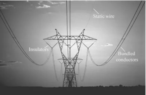
A transmission grid is a network of power stations, transmission lines, and substations. Energy is usually transmitted within a grid with three-phase AC. Transmission lines are either overhead power lines or underground power cables. Overhead cables are not insulated and are vulnerable to the weather but can be less expensive to install than underground power cables. Overhead and underground transmission lines are made of aluminum alloy and reinforced with steel; underground lines are typically insulated. Figure 2 shows a three-phase 500 kV transmission line with two conductors per phase. The two conductors per phase option is called bundling. Multiple conductors are bundled together per phase to double, triple, or greater to increase the power transport capability of a power line, lower losses and improve other operating characteristics of the line such as electromagnetic fields and audible noise.

Typically, there are three types of line configurations used in the transmission network. These line configurations include (a) radial (one-terminal), (b) two-terminal, and (c) multi-terminal of which three-terminal is possibly the most prominent multi-terminal type. It should be noted that "terminals" in this context, refers to source terminals and not-tapped transformer terminals or stations. The two-terminal line configuration is the most dominant type followed by radial, and the three-terminal lines are the exceptions.

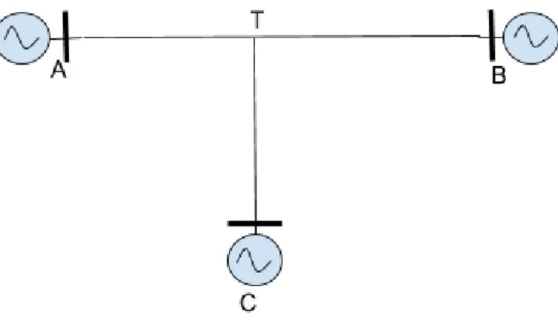
Three-terminal systems are used in power transmission networks to connect three power sources, A, B, and C. The power sources are either generators or Thevenin equivalent of a

(17)

connected network. As shown as in Figure 3, the three terminals are connected through a Tap-point T which does not contain any measuring devices. Protection systems are like that of two-ended lines except with more sophisticated techniques. In many cases, an existing two-terminal line is converted to three-terminal line as part of program to reinforce the power system. At least one (generally two) communications-based protection groups are normally used with three-terminal line applications.

Figure 3: Three-terminal Transmission Lines

Two-terminal line systems are used for bulk power transfer and to supply loads from two power sources- Terminals A, B and are very common. Figure 4 shows the two-terminal transmission line. To obtain proper selectivity and coordination, directional distance relays [6] for phase and ground fault detection are used normally. Directional ground overcurrent relaying is sometimes applied in addition to, or in place of, directional ground distance relay functions. One or two communications-based protection groups are normally used with two-terminal line applications at the transmission voltages greater than 200KV.

Figure 4: Two-terminal Transmission Line

Radial lines are lines that supply loads from single power source- Terminal A as shown in Figure 5. Nondirectional overcurrent or distance relays are normally used to protect these types of

(18)

lines. Communications based tripping is not generally necessary.

Figure 5: Radial Configuration

1.4 Problem Statement

Transmission lines or transmission network is a crucial part of the electric grid as it carries high voltage power from generating site to the substations where the voltage stepped-down for end-use consumption transported via distribution lines. Though the frequency of faults is much higher in distribution lines, faults on transmission lines have more widespread impact and faults in buried transmission lines take longer to locate and repair. Additionally, since the transmission lines carry high voltages, faults on these lines might lead to unsafe conditions. Therefore, safeguarding against exposed fault is the most critical task in the protection of power system. The protection schemes or mechanisms for the transmission lines become challenging as configurations of the transmission lines become increasingly complex.

Three-terminal and other multi-terminal line construction are generally a trade-off of planning economics and protection complexities. Two-terminal lines with long tap(s) supplying remote load from the main line may display many of the same protection and load ability issues as three-terminal lines. The complexity of protecting these line configurations increases from the relatively simple radial, to the more difficult two-terminal, and to the still more difficult three-terminal. Relaying three-terminal lines has been and continues to be a challenge for protection engineers [7].

Primary and biggest challenge with protecting three terminal circuits is “Infeed”. During a fault on the transmission line, distance relay measures impedance which is equal to the positive sequence (A balanced three-phase system with the same phase sequence as the original sequence), if there are no sources of fault current on the transmission line between the line terminal where the relay is located and the fault.

(19)

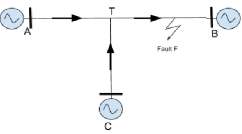
Figure 6: Infeed Effect at Three-terminal

From the Figure 6, the actual line impedance from the relay terminal (Terminal A) to the fault is not always the impedance measured by the relay. This is because the third line terminal (Terminal C) tapped (Tee point) to a line is an additional source of current for a line fault. Current will be supplied to a fault that occurs on the line section beyond the tap of Terminal C through both Terminal A and Terminal C. The voltage drops resulting from the input of fault current from each of these sources into the common section of the line will be measured by the distance relay at the Terminal A. Since the current input from Terminal C is not applied to the relay at Terminal A, the impedance measured by this relay is higher than the actual impedance from the Terminal A to the fault. The relay will under reach; that is, for a given relay setting the relay does not cover the same length of line it would if the additional current source were not present. Due to infeed, most of the impedance based and traveling wave-based methods are not successful in identifying faults and often give erroneous results [8].

(20)

It is also possible to experience an “Outfeed” at the T location, in which case there will be

tendency to overreach as shown in

Figure 7. This phenomenon is not too common but can cause delayed or sequential tripping at the terminals.

Thirdly, transmission lines could traverse long distances, in which case the line A-B ends up being in one region and line C-T in different region with separate set of environmental conditions which directly influences the impedance of the respective lines. This causes line non- homogeneity and since impedance on line C-T is different that of line A-B which makes fault location on line C-T trickier. Therefore, there is a need of an adaptable, resilient method for fault classification and location on transmission lines which could learn from system behavior and detect unknown faults rather than hardcoded methods (algorithms)which follow specific set of rules.

Taken all together, faults on transmission lines and the varying environmental conditions present a complex classification and detection problem. With the advent of new machine learning methods and supervised learning methods, these challenges may be more effectively addressed. Machine learning methods are based on the idea that systems can learn from data, identify patterns and make decisions with minimal human intervention. The ability to automatically apply complex mathematical calculations to big data – over and over, faster and faster give these algorithms potential to identify insights in the data which would be otherwise an impossible task for humans. The availability of high-resolution/high-volume data, due to the proliferation of intelligent electronic devices in smart grids, paves ground to implement more accurate and intelligent machine learning methods for fault classification and location identification on the transmission lines.

1.5 Contributions and Thesis Outline

Majority of the faults on the transmission lines are shunt faults and with around 5% of them being symmetric (all three phases are equally affected). This research presents supervised-learning method for classification and location of shunt faults on three-terminal and two terminal transmission lines. The main contributions of the research are:

(21)

● Two different architectures are proposed which adapts to any N-terminal in the transmission line (dimensional scaling).

● The models proposed do not require large dataset or high sampling frequency. Additionally, they can be trained quickly and generalize well to the problem.

● The first architecture is based off decision trees for its simplicity, easy visualization which have not been used earlier. In this instance, fault location method uses traveling wave-based approach for location of faults. The method is tested with performance better than expected accuracy and fault location error is less than ±1%.

● The second architecture uses single Support Vector Machine to classify ten types of shunt faults and Regression model for fault location which eliminates manual work. The architecture was tested on real data and has proven to be better than first architecture. The regression model has fault location error less than ±1% for both three and two terminals.

● Both the architectures are tested on real fault data which gives a substantial evidence of its application.

The thesis is organized into 5 chapters. Chapter 2 discusses relevant literature and presents a survey of different machine learning methods proposed over past years. The two new architectures for fault classification and location is proposed in Chapter 3. Chapter 4 details the experimental setup, implementation and results are presented. Chapter 5 summarizes the conclusions and proposes the possibilities of future work.

(22)

Chapter 2 : Background and Related Work

2.1 Introduction

Given the electrical power grid is a complex power system consisting of power generating stations, high voltage transmission lines and distribution lines, fault classification and location identification is necessary to improve protection mechanisms and have reliable, high-speed protection devices. Most often, electrical faults result in mechanical or material damage to the lines or structures, which must be repaired before returning the line to service. As it is noted earlier, repair and restoration is extremely important for maintaining critical and societal services. The restoration process is hampered if the location of the fault cannot be estimated with accuracy or confidence (less than a mile). Various methods have been proposed over the years, and each method have their own merits and disadvantages.

Section 2.2 presents an overview on several types of electric faults occurring on transmission lines. In Section 2.3, to encapsulate the current state of art methods, a survey review is presented on popular machine learning algorithms used for fault classification and location on transmission lines and summaries are given in Section 2.4.

2.2 Review of the Faults on the Transmission Line

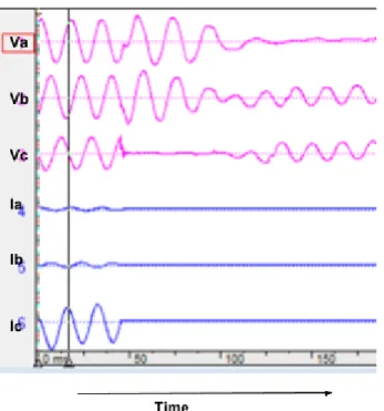
In an electric power system, a fault or fault current is any abnormal electric current. For example, a short circuit is a fault in which current bypasses the normal load and an open-circuit fault occur if a circuit is interrupted by some failure. Transmission line carry 3-phase AC [9]. Under ideal state, all phase voltages have same maximum value but differ in phase from each other at angle 120 degrees. Shunt faults are caused by short circuit between lines. For example, a line to ground fault occurs when one conductor drops to the ground or comes in contact with the neutral conductor (ground). This causes a rapid decrease in respective phase voltage of the line involved in the fault and increase in phase current. Figure 8 shows the phase C-to-ground fault in time (µs).

𝑉_𝑎, 𝑉_𝑏, 𝑉_𝑐 are the phase voltages of phase a, b, c and 𝐼_𝑎, 𝐼_𝑏, 𝐼_𝑐 are the phase currents of phase a, b, c respectively. From the figure we can see that, magnitude of phase C voltage decreases and phase

(23)

C current increases during the fault.

Figure 8: Phase to ground fault in time

Faults can be categorized as the shunt faults and series faults [10] described below:

2.2.1 Series Faults

Series faults represent open conductor and take place when unbalanced series impedance conditions of the lines are present. These faults disturb the symmetry in one or two phases and are therefore unbalanced faults. Two examples of series fault are when the system holds one or two broken lines, or impedance inserted in one or two lines. In the real world a series faults takes place, for example, when circuit breakers control the lines and do not open all three phases, in this case, one or two phases of the line may be open while the other/s is closed [10]. Series faults are characterized by increase of voltage and frequency and fall in current in the faulted phases.

(24)

2.2.2 Shunt Faults

Figure 9:Classification of Short Circuit faults

There are two types of short circuit faults or shunt faults which can occur on transmission lines; balanced faults and unbalanced faults also known as symmetrical and unsymmetrical faults respectively as shown in Figure 9. In symmetrical faults, also called three phase short circuits, all the three phases are short circuited to each other and often to earth also. Such faults are balanced and symmetrical as the system remains balanced even after the occurrence of the fault. Though the symmetrical faults are rare, they generally lead to the most severe fault current flow. Most faults that occur in a power system are unsymmetrical faults involving only one or two phases. The most common type of unsymmetrical fault is a short circuit between a phase and the earth.

The shunt faults are the most common type of fault taking place in the field. They involve power conductors or conductor-to-ground or short circuits between conductors. One of the most important characteristics of shunt faults is the increment the current suffers and fall in voltage and increase frequency. Shunt faults can be classified into four categories [11].

1. Line-to-ground fault: This type of fault exists when one phase of any transmission lines establishes a connection with the ground either by ice, wind, falling tree or any other incident. About 70% of all transmission lines faults are classified under this category [12].

1. Line-to-line fault: Because of high winds, one phase could touch anther phase & line-to-line fault takes place. Approximately 15% of all transmission lines faults are considered line-to-line faults [12].

2. Double line-to-ground: Falling tree where two phases become in contact with the ground could lead to this type of fault. Two phases will be involved instead of one

(25)

in the line-to-ground faults scenarios. Ten percent of all transmission lines faults are under this type of faults [12].

3. Three phase faults: In this case, falling tower, failure of equipment or even a line breaking and touching the remaining phases can cause three phase faults. In reality, this type of fault not often exists which can be seen from its share of 5% of all transmission lines faults [12]. The first three of these faults are known as asymmetrical faults.

2.3 Survey of the methods

This section presents a survey on different fault classification and location identification techniques in transmission lines highlighting the implementations machine learning methods in the past. In this review, only short circuit faults are considered as they are more common.

Figure 10: Fault detection techniques

The survey is mainly divided into two parts:

1) Fault classification techniques - Methods that determine the fault type 2) Fault Location Techniques - Methods that calculate the distance of the fault

Both techniques play a vital role in development of protection mechanisms for a given power system model. There have been various approaches used to develop a fast speed and reliable method to deal with faults as shown in Figure 10.

(26)

Wavelet based approaches primarily use the time difference between the traveling wave reflections which assume higher sampling rate and synchronized measurements at the terminals for fault identification making it difficult for a practical application, especially for three-terminal circuits due to infeed problem. Though this method has lower error of estimation, it has a higher computational burden [13]. Phasor measurement unit (PMU) based approaches require synchronized phasor quantities from all the terminals of the transmission lines. Genetic Algorithms are the heuristic search and optimization techniques that mimic the process of natural evolution. When applied to classify and location faults on transmission lines, they are often slow and complex to be implemented [14].

Machine learning is a subset of artificial intelligence in the field of computer science that often uses statistical techniques to give computers the ability to "learn" (i.e., progressively improve performance on a specific task) with data, without being explicitly programmed [15]. Machine learning algorithms can learn and improve themselves by studying high volumes of available data. They are very helpful in fields where traditional programming rules do-not operate or rules keep evolving. Since the faults occurring on power grid are very unlikely to be similar and power system can change depending on the future demand, use of machine learning algorithms for solving such problems might. They can benefit from learning correlation between events and can give insights helping human uncover factors causing the faults and to find the solution of complex multiobjective nonlinear systems, the above-said methods are used to get faster solution and less error.

2.3.1 Fault Classification Techniques- Machine Learning

Classification of power system faults is the first stage for improving power quality and ensuring the system protection. For this purpose, a robust classifier is necessary.

Most prominent machine learning approaches for fault classification are explained below:

A. Support Vector Machines (SVM)

Support Vector Machines are supervised learning models which maps the high dimensional input space to target space [16]. The main advantage is its regularization parameter, it tells the SVM to avoid misclassifying each training sample [17]. Secondly, SVM works well with continuous data and can learn more from less number of samples. Section 3.3.1 describes the SVM

(27)

in more detail.

One promising indicator is that researchers in the past have used SVM for as a classifier to carry out fault classification in the transmission lines [13]. Babu et al. [18] proposed fault

classification using Empirical Mode Decomposition (EMD) and SVM’s. EMD was used to

decompose the voltages of transmission line into Intrinsic Mode Function (IMF’s). The characteristic features from the IMF’s were extracted by Hilbert Huang Transform which was given as input to three SVM’s trained for three phases respectively to predict their involvement in

the fault. The method was tested on the simulated data with acceptable levels of accuracy.

K. Li et al. [19] presented fault detection and classification method based on Principal Component Analysis (PCA) and SVM. In the first step, PCA is used to reduce the dimensionality as well as find violating point of the signals according to the confidential limit. In the second step, extracted features are used to build SVM networks to use the pattern recognition to identify faulty phase. However, the PCA cannot identify non-linear relationships which might not work well with three-terminal circuits.

Malathi et. al [20] proposed an approach for fault classification in transmission line using multi-class Support Vector Machine (SVM). Wavelet decomposition using Discrete Wavelet Transform (DWT) of post fault phase current signals are used as a feature set for the SVM which predicts the fault class. This method has been tested extensively on various simulated conditions on the transmission line with different network conditions.

Dubey et. al. [21] used proposed fault classification method using Least Square SVM (LS-SVM). The main advantage of this method is that it requires lesser training sets. Post fault one-fourth cycle current signal is used as input to four LS-SVM, for prediction of three phases and ground respectively. The results have been validated on the simulated data under various fault conditions.

An approach of combining Discrete Wavelet Transform (DWT) with SVM for fault classification was proposed by Hanif et. al. [22]. DWT is used to extract the post fault voltage energies and normalized energies are used as input to the four SVM classifiers used to predict the involvement of each phase in the fault. The method was evaluated using simulated data for two different networks; an overhead line combined with an underground cable and a 6-bus distribution network.

(28)

Youssef et. al [23] proposed approach to detect and classify faults in real-time using SVMs. The main idea is to use fault inception angle as input to SVM to recognize the patterns. Phase angle after the fault were recorded for nine types of fault types and used to train the two SVMs.

There have been researches implementing SVM for detecting and classifying faults on series compensated circuit [24]–[26] which is out of boundaries for this research.

B. Neural Network

Artificial Neural Networks are computing systems vaguely inspired by the biological neural networks that constitute animal brains. An ANN is based on a collection of connected units or nodes called artificial neurons which loosely model the neurons in a biological brain. Each connection, like the synapses in a biological brain, can transmit a signal from one artificial neuron to another. An artificial neuron that receives a signal can process it and then signal additional artificial neurons connected to it. The original goal of the ANN approach was to solve problems in the same way that a human brain would. Figure 11 shows an artificial neural network which is an interconnected group of nodes, akin to the vast network of neurons in a brain. Here, each circular node represents an artificial neuron and an arrow represents a connection from the output of one artificial neuron to the input of another. However, over time, attention moved to performing specific tasks, leading to deviations from biology. Many researches have used neural network for fault classification and detection explained in [27].

(29)

Figure 11: Artificial Neural Network [28]

Koley et. al. [29] proposed a hybrid wavelet transform and modular artificial neural network based fault detector, classifier and locator for six phase lines using single end (single terminal) data. The standard deviation of the approximate coefficients of voltage and current signals obtained using discrete wavelet transform are applied as input to the modular artificial neural network for fault classification and location.

Ahmad et. al. [30] proposed wavelet based artificial neural networks for fault classification. Discrete wavelet transforms (DWT) is used to extract high-frequency components of the aerial modal currents. A feature vector is built using the wavelets details coefficients of one level of the aerial modes and is used to train an ANN. The proposed method is tested on the simulated data with acceptable accuracies.

Rao et. al. [31] has presented a fault classification and detection method using discrete wavelet transform and artificial neural networks. Discrete wavelet Transform (DWT) is applied to the fault phase currents to obtain energy values which is used as input to train the neural network. The proposed method was tested on a simulated network values using MATLAB.

Few other researchers have used Back-Propagation Neural Network (BPNN) for identifying and classifying faults on transmission lines. Backpropagation is a method used in

(30)

artificial neural networks to calculate a gradient that is needed in the calculation of the weights to be used in the network. It is commonly used to train deep neural networks, a term referring to neural networks with more than one hidden layer.

Saini et. al. [32] has proposed new algorithm for fault detection and classification on parallel transmission lines using Discrete Wavelet Transform (DWT) and Back-Propagation Neural Network (BPNN). Wavelet energies coefficients of alpha and beta mode currents obtained by clark’s transformation are used as input to train BPNN with two hidden layers. The proposed

method is tested on different networks and fault scenarios.

C. Fuzzy Logic

Fuzzy logic is a form of many-valued logic in which the truth values of variables may be any real number between 0 and 1. It is employed to handle the concept of partial truth, where the truth value may range between completely true and completely false. By contrast, in boolean logic, the truth values of variables may only be the integer values 0 or 1. They do not need detailed knowledge of the system as the decisions are based on rules determined by humans. Figure 12 shows the basic building block of a fuzzy scheme consisting of 3 stages. In the fuzzification, the inputs (for fault classification voltage/current transients) fuzzified into fuzzy membership functions. In the Fuzzy Inference System, all the rules in the rule base are used to compute the fuzzy output functions. De-fuzzification stage, maps the fuzzy output functions to get predicted fault type.

Figure 12: Block Diagram of Fuzzy Logic System

Saradarzadeh et. al. [33] proposed an algorithm for fault type recognition of shunt faults that occur on the transmission line. The proposed method uses the phase sequence components of three phase voltages and currents that are available in most of the power system protection relays.

(31)

A fuzzy method is used to identify the type of fault from the current and voltage signals separately and then combines the results to provide more accurate fault-type recognition.

Prasad et. al. [34] proposed a method for fault classification. Post fault currents from three phases of one terminal is used as input to the Fuzzy Inference System (FIS) to classify faults. The proposed technique using two classifiers one is for ground faults (Fuzzy classifier-I) and second one is for phase faults (Fuzzy classifier-II). The method is tested on the simulated network.

Adhikari et. al. [35] used three phase currents data obtained from Compact Reconfigurable i/o (CRIO) devices as input to their method using Fuzzy logic. Once the rule base is prepared for classification, compiled fuzzy logic is dumped to FPGA (field-programmable gate array) to get a real-time performance.

D. Other Techniques

The other machine learning techniques used in fault classification and identification. Jamehbozorg et. al. [36] proposed Decision Tree based method for fault classification in Double-Circuit Transmission Lines. The proposed method needs voltages and currents of only one terminal of the protected line. After detecting the exact time of fault inception and calculating the odd harmonics of the measured signals, up to the nineteenth, a decision tree algorithm is employed for recognition of the intercarrier fault type. Also, the proposed method is extended for classification of crossover faults in these transmission lines.

Mishra et. al [37] have used bagged tree ensemble technique. Bagging stands for bootstrap aggregation; whereby random samples are drawn through replacing the training datasets. Bagging is a simple method that can be employed to reduce the variance for those machine learning techniques with high variance. Post fault current is decomposed by Fast Discrete Orthonormal S-Transform (FDOST) and bagged tree ensemble technique is used to classify faults. The proposed method is then tested under different fault scenarios on the simulated data.

K-Nearest Neighbor (k-NN) based classification method was proposed by Majd et. al. [38]. Distances of each sample and its fifth nearest neighbor in pre-determined in the default window which determines the fault occurrence time and phase. Therefore, k-NN is applied to the instantaneous values of normalized three phase currents.

(32)

technique in a series compensated transmission line. Extreme learning machines are feedforward neural networks for classification, regression and feature learning with a single layer or multiple layers of hidden nodes, where the parameters of hidden nodes (not just the weights connecting inputs to hidden nodes) need not be tuned. Discrete Wavelet Transform (DWT) is used to decompose the instantaneous current signals used as input to ELM for fault classification. The proposed method is tested with simulated data.

Dasgupta et. al. [40] proposed a method for detecting and classifying transmission line faults using cross-correlation and k-Nearest Neighbor (k-NN). This method computes the cross correlation between pure and faulty current signals. Extracted features are used as input the k-NN algorithm which then computes distance of a given sample to all other samples in the set and class of the sample with least distance is predicted.

Linear Regression Index-Based Method for fault classification and detection is presented by Musa et. al. [41]. The proposed algorithm has constructed a rule as follows: when the system is running under healthy condition, the Linear Regression Coefficient Indices (LRICs) will be equal to zero; when the system is subjected to the fault condition, the LRICs of faulted phases will be greater than zero. For each possible scenario of faults, the proposed algorithm required only the three-phase current measurement of the local measurement.

2.3.2 Fault Location Techniques

–

Machine Learning

Accurate fault location that occur on transmission lines is highly important from aspect of quick identification of weak points on the transmission line and taking respective counter measures to decrease the probability of those faults. Various approaches have been developed over the time to address these issues and in those few are hard coded. On the other hand, power of algorithms which can learn from real world pattern are explored. Figure 10 shows few fault location techniques that have been developed by the researches in the past. In this section, machine learning techniques employed in past have been summarized.

A. Neural Networks

Neural Networks becomes first choice when the goal is to model non-linear and complex relationships which follow real-life pattern. They generalize well which results in a model that

(33)

Twafik et. al. [42] proposed Artificial Neural Network (ANN) for estimating fault location on transmission lines. Prony method is used to extract the modal information from voltage or current signal. ANN are then used to estimate the fault distance based on the modal information. The model is trained and tested using the simulated data.

Fathabadi et. al. [43] proposed an hybrid framework consisting of a proposed two stage Finite Impulse Response (FIR) filter, four Support Vector Machines (SVMs), and eleven Support Vector Regressions (SVRs). The proposed two-stage FIR filter together with the SVMs are used to detect and classify short-circuit faults while the SVRs are utilized to locate short-circuit faults and predict distances.

Yadav et. al. [44] have written a comprehensive and exhaustive survey will reduce the difficulty of new researchers to evaluate different ANN based techniques with a set of references of all concerned contributions. From the survey they concluded that ANN is found to be robust, accurate, and efficient approach for transmission line fault detection, classification, localization, direction discrimination, and faulty phase selection.

B. Support Vector Regression (SVR)

The Support Vector Regression (SVR) uses the same principles as the SVM for classification. Because output is a real number it becomes very difficult to predict the information at hand, which has infinite possibilities. In the case of regression, a margin of tolerance (epsilon) is set in approximation to the SVM which would have already requested from the problem.

Ray et. al. [45] proposed Support Vector Machine (SVM) for fault classification and Support Vector Regression (SVR) for fault location. Fault classification consists of four SVMs each predicting the involvement of each phase and fault location consisting of SVR. Both the models have been trained by best features out of decomposed post fault current signals using Wavelet packet transform (WPT). The proposed method has been trained and tested on the simulated data and a comparison study has been carried out with methods published by other researchers.

Hosseini et. al. [46] presented hybrid method for fault classification and location. Post fault voltage samples are decomposed by discrete wavelet transform which are used with post fault current samples as input to SVM for the fault classification model. Four SVMs are used to predict

(34)

the fault in each phase. Depending on the fault type in the first stage, the second stage one out of four SVRs is selected for fault location.

C. Other Techniques

Farshad et. al. [47] proposed a method to classify and locate single-to-ground faults using k-Nearest Neighbors (k-NN) algorithm. Various features are extracted from the voltage signals measure from a single terminal. Decomposed signals from the discrete Fourier Transform is used as input to k-NN for fault type classification. k-NN in regression mode is used for fault location. Since, current signals are not used, the proposed approach is immune against current-transformer saturation and its related errors.

Ray et. al. [48] in proposed fault location technique using extreme learning machine (ELM) in series compensated transmission line. The proposed method uses one cycle of post fault current and voltage signals which are decomposed by wavelet transform. Best features, selected by genetic algorithm are then used as input to the ELM. The method has been tested on variety of simulated data.

2.4 Summary

Variety of approaches have been used to increase reliability and robustness of fault classification and location methods.

Neural Network follows a black box model making the explanation for the result typically difficult to understand. Neural network-based fault classification methods show good accuracy, however the training time is quite large due to which the task becomes more complex. The artificial neural network techniques suffer from the requirement of large training data. However, these

methods are hard to implement practically. If the fault can’t be identified quickly, it will produce

many ill-effects such as line outages during the period of peak load leading to severe economic losses. There may be a chance for the entire grid to collapse which is called as blackout and the reliability of the system would be affected.

Few of the fault classification and location methods use fuzzy logic based architectures [13]. Fuzzy logic uses rule-based relationship for making decisions. Though they have lot less computation burden, it is tedious to develop fuzzy rules and membership functions and fuzzy

(35)

outputs can be interpreted in many ways making analysis difficult. In addition, it requires lot of data and expertise to develop a fuzzy system.

Other impedance measurement-based methods for fault location depend on fundamental concept of calculating line impedances pre- and post-faults to determine the distance of the fault. However, in three terminal circuits, due to infeed, the impedance values are measured are much larger than actual line impedance which gives rise to erroneous results. Secondly, the lines A-B and C-T may be in different terrains which results in different environmental conditions. In this scenario, synchronized impedance measurements might provide erroneous results.

It appears, Current state of the art Machine Learning methods presented in above sections have tested models on simulated data which have same distribution, pattern/trend as training data. Therefore, the robustness of the methods is not completely known and the question of whether these methods are applicable to 3 terminal networks is yet to be answered.

(36)

Chapter 3 : Design

3.1 Introduction

In the recent past, many researchers have proposed approaches for fault classification and location identification. However, they were not applicable to a variety of transmission network configurations, particularity 3 terminal networks and were not evaluated with real data to ensure the effectiveness of the methods in locating and classifying faults on the transmission line.

Based on the literature review and preliminary designs, the design criteria that emerged is as follows:

1. Scalability. Transmission network expand as the demand for the power increases every year. Therefore, fault location methods should be scalable.

2. Confidence. Should produce estimates that are timely, sound and reliable, otherwise the confidence in the methods would be weakened and longer lengths of transmission line would have to be examined to find the exact fault location.

3. Network Topology. Adaptive to different configurations, applicable to changing fault data.

4. Relevant. Make use of existing power line health data

5. Extensible. Interface with existing OT power line monitoring devices.

Based on recent advances in machine learning, it was decided to explore the utility and applicability of machine learning to fault classification and location on transmission lines. Machine learning is a form of data analysis that automates analytical model building [49]. Using algorithms that continuously assess and learn from data, machine learning algorithms enables hidden insights into complex behavior and relationships. It can handle multi-dimensional and multi-variable data

in dynamic environments. A key aspect to machine learning algorithms is that they learn the behavior of the system representative and synthetic datasets to produce reliable, repeatable decisions and results. For fault classification and location on transmission lines, these attributes are desirable. In addition, machine learning methods do not require synchronized measurements at the terminals. Additionally, they can be employed in real time to monitor the grid as well.

(37)

Input data is very crucial aspect for the machine learning algorithms and the correctness of prediction is based on the quality of data that the model was trained with. Post- fault voltage or current transients from the live grid are prone to have small amount of noise (may be negligible). Therefore, to ensure the quality of the data used to train the machine learning models and to extract required features from the post-fault signal, Discrete Wavelet Transform (DWT) is used. The advantage of DWT lies in determination of the key components in the signal like energy and entropy. The training data which consists of these components is used to train the predictive models so that they can learn from the information given by these components.

In predictive modeling, the idea is to create a function which is isomorphic to original function/process which was used to generate the training data. Therefore, this predictive model can predict new data points using the “new” function. The fault type and faulty line identification on the transmission line is a classification problem – in which we want to build a classification model to classify ten fault types into the target classes. Based on the preliminary research, we focused on two machine learning based architectures. The first architecture employs decision trees and second architecture use multi-class Support Vector Machines (SVM) for fault classification and faulty line identification. Both SVM and Decision trees follow white box ( subsystem whose internals can be viewed but usually not altered) approach and are capable of handling continuous data (floating point).

Section 3.2 gives the details about the overall process for fault identification in the transmission lines.

3.2 Overview

Figure 13: High Level Overview of the Process

This section provides an overview of the proposed method as shown in Figure 13. The goal is to employ machine learning methods to identify faults and fault location on a given transmission line or circuit rather than hard coding the values.

(38)

The process has mainly three major steps below:

1) Data Generation: The machine learning algorithms need to be trained before deployment in real time to detect faults and identify locations. In this step, simulated data of fault phase voltages is collected from an emulated Transmission model resembling the live transmission model. The collected data then is normalized and massaged before it can be used as training data to train the models. 2) Fault Type Identification: The goal is to correctly classify ten types of Short circuit faults as described Chapter 2. Two different architectures are presented in the later sections consisting machine learning algorithms to predict the fault type.

3) Fault Location Identification: The methodology differs for three terminals and two terminal circuits. Fault location identification in first architecture is using wavelet-based traveling wave method to calculate the distance. The second method is to employ regression models to predict the distance of the fault.

Section 3.2 describe the data generation process in detail. Section 3.3 and 3.4 present two different architecture for fault type classification and location methods.

3.3 Data Generation

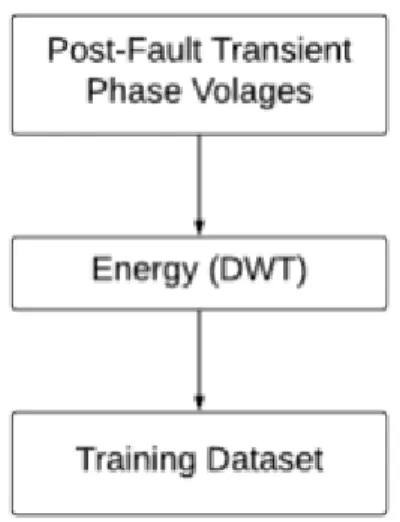
Data Generation is a crucial step to any method employing machine learning algorithms. The algorithm or model needs to be trained beforehand to predict the outcome for the test sample. The model is initially fit on a training dataset that is a set of examples used to fit the parameters of the model and tested on the test dataset which is used to provide an unbiased evaluation of a final model fit on the training dataset. Machine learning algorithms learn from data. Therefore, it is critical that you feed them the appropriate data for the problem being addressed. Additionally, the type of the data collected governs the choice of machine learning algorithm to be applied to obtain best results. For the fault classification and location problem, the data generation process is presented in Figure 14.

(39)

Figure 14:Data Generation Process

It is a three-step process provided as follows:

1) Post fault transient three phases (Va, Vb, Vc) and ground mode voltages are recorded for

one cycle on each terminal of the transmission model under study. Simulated post fault transient voltages from all the terminals is obtained from simulating the faults on the network using Aspen One-liner [50]. Post fault transient phase current value also could be used in place of phase voltages which is to be tried in future work.

2) Discrete Wavelet Transform is applied to the transient phase and ground mode voltages to get the wavelet transform approximation coefficients (WTAC’s). To minimize noise effect wavelet coefficients are squared [51]. Energy of the wavelet is obtained by summation of all the 𝑊𝑇𝐴𝐶2_{over one cycle after the fault has occurred.}

𝐸𝑚= ∑ 𝑊𝑇𝐴𝐶2(𝑘) ∀ 𝑚 ∈ {𝑎, 𝑏, 𝑐 𝑎𝑛𝑑 𝑔} 𝑎𝑛𝑑 𝑘 ∈ {0, 𝐾 − 1 𝐾−1

𝑘= 0

} Where K is the number of cycles

The obtained wavelet energies are normalized as 𝐸𝑁𝑘=

𝐸𝑚

𝐸𝑚𝑎+ 𝐸𝑚𝑏+ 𝐸𝑚𝑐+ 𝐸𝑚𝑔

∀ 𝑚 ∈ {𝑎, 𝑏, 𝑐 𝑎𝑛𝑑 𝑔}

3) The input features are calculated wavelet energies at all the terminals. For three terminal models, the data set consists of wavelet energies from all the three terminals A, B and C. Classification of fault is done from the obtained energy of the approximation coefficients.

(40)

4) For architecture I, the number of target labels to be predicted is 4, phase A, B, C and Ground. Therefore, three-terminal training set would be Nx12 matrix features and Nx4 target labels, where N is the number of samples in the dataset. Two terminal has Nx8 feature matrix and same target labels. For architecture II, the feature space for two and three terminals does not change, the target matrix reduces to Nx1.

All the machine learning algorithms are trained with above training simulated dataset. Once the training is done, the algorithms will have optimal decision boundaries which will be used to predict the outcome of the real-time fault during the testing phase.

The next section briefly describes Discrete Wavelet Transform (DWT) and then the later sections present the proposed architectures.

3.3.1 Discrete Wavelet Transform

A discrete wavelet transform (DWT) is any wavelet transform for which the wavelets are discretely sampled. For fault classification and location technique, DWT is a method of preparing the data. Traveling wave theory is utilized in capturing the travel time of the transients along the monitored lines between the fault point and the relay. Time resolution for the high frequency components of the fault transients, is provided by the wavelet transform. Using wavelets for fault location was first proposed in [52].

Traveling wave or ultra-high-speed fault location method utilizes the higher frequency contents of the transient fault signals due to its use of traveling wave theory and shorter sampling windows.

Wavelet transform possesses some unique features that make it very suitable for this application. It maps a given function from the time domain into time-scaling domain. The wavelet, the basis function used in the wavelet transform, has bandpass characteristics which makes this mapping like a mapping to the time-frequency plane. The wavelet transform is often compared with the Fourier transform, in which signals are represented as a sum of sinusoids. In fact, the Fourier transform can be viewed as a special case of the continuous wavelet transform with the choice of the mother wavelet (𝑡) = 𝑒−2𝜋𝑖𝑡_{. The main difference in general is that wavelets are}

localized in both time and frequency whereas the standard Fourier transform is only localized in frequency. This localization allows the detection of the time of occurrence of abrupt disturbances,