A Simple Component Connection Approach for Fault Tree Conversion to Binary

This item was submitted to Loughborough’s Institutional Repository by the

author and is made available under the following Creative Commons Licence

conditions.

For the full text of this licence, please go to:

A Simple Component Connection Approach for Fault Tree Conversion to Binary

Decision Diagram

R. Remenyte;

Department of Aeronautical and Automotive

Engineering

Loughborough University; Loughborough,

Leicestershire, England

e-mail: [email protected]

J.D. Andrews;

Department of Aeronautical and Automotive

Engineering

Loughborough University; Loughborough,

Leicestershire, England.

e-mail:

[email protected]

Abstract

Fault Tree Analysis (FTA) is commonly used when conducting risk assessments of industrial systems. A number of computer packages based on conventional analysis methods are available to perform the analysis. However, dealing with large (possibly non-coherent) fault trees can expose the limitations of the technique in terms of accuracy of the solutions and the processing time required. Over recent years the Binary Decision Diagram (BDD) method has been developed for the solution of the fault tree and overcomes the disadvantages of the conventional FTA approaches. The usual way of taking advantage of the BDD structure is to construct a fault tree and then convert it to a BDD. This paper will focus on the fault tree to BDD conversion process.

Converting the fault tree requires the basic events of the fault tree to be placed in an ordering. This is critical to the size of the final BDD and ultimately affects the qualitative and quantitative analysis of the system and benefits of this method. Once the ordering is established several approaches can be used for the BDD generation. One approach is to apply a set of rules developed by Rauzy which are repeatedly applied to each gate in the fault tree to generate the BDD. An alternative approach can be used when BDD constructs for each of the gate types are first built and then connected together. A sub-node sharing feature in the second of these approaches and a third, hybrid, combined approach will be presented. Some remarks on the effectiveness of these techniques will be provided.

1. Introduction

The Binary Decision Diagram (BDD) method [1] has been developed as an approach for the analysis of fault trees. This method has been shown to have advantages in

terms of both efficiency and accuracy over the conventional Kinetic Tree Theory [2], since top event probabilities can be derived without the need for approximation and also without the need to evaluate the minimal cut sets as intermediate results.

The BDD method first converts the fault tree to a binary decision diagram, which represents the Boolean equation for the top event. Problems may occur with the conversion process of the fault tree to the BDD. If the ordering of the basic events is not chosen suitably, the size of the final BDD can grow exponentially. It is impossible to identify an optimum ordering scheme for producing BDDs for all fault trees. In this paper alternative conversion methods are presented. These include new methods where BDDs for each of the gate types are formed and then joined together according to the type of the parent gate in the fault tree.

The efficiency of the alternative approaches is compared with the conventional method developed by Rauzy [1]. Three efficiency measures are applied while looking for the optimum connection technique. A sub-node sharing approach is introduced to the component connection method during the connection process, together with the development of the hybrid approach utilising the advantageous rules of both approaches.

2. Binary decision diagram method

A BDD is a directed acyclic graph, as shown in Figure 1. All paths through the BDD start at the root vertex and terminate in one of two states – a 1-state (system failure), or a 0-state (system success). The BDD is composed of terminal and non-terminal vertices, which are connected by branches. Terminal vertices correspond to the final state of the system and non-terminal vertices correspond to the basic events of the fault tree. By connection, all left branches leaving a vertex are the 1-branches (component

fails), all right branches are the 0-braches (component functions).

Figure 1. Example of BDD

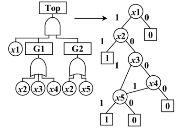
The BDD encodes the logic function of the system failure in its disjoint form. In the example of a fault tree and its equivalent BDD shown in Figure 2 the logic function is:

Top =x1·(x2 + x3)·(x2 + x4) = x1·x2 + x1·x3·x4 [1] where “+” represents Boolean operator OR, “·” represents Boolean operator AND.

Figure 2. Example FT converted to BDD, ordering x1 < x2 < x3 < x4

In the BDD shown in Figure 2 there are two possible paths that terminate in a 1 state:

2 , 1 x

x andx1,x2,x3,x4 [2] Each path describes a combination of component conditions where the existence of all of them will result in system failure. These two paths, when considering only the failure events, give the two cut sets:

{x1,x2} and { x1,x3, x4}. [3] Only the vertices that lie on the 1 branches of the paths

are included in the cut sets. The cut sets obtained are minimal (they contain necessary and sufficient elements), since the BDD in this example is in its minimal form. Otherwise, the BDD has to undergo a minimisation procedure, introduced in [1], in order to obtain minimal cut sets.

The probability of occurrence of the top event, Q_SYS, can be expressed as the sum of the probabilities of the disjoint paths through the BDD, since paths through the

BDD are mutually exclusive. The probability of system failure in the example is:

(

2

)

3 4 1 2 1 x x 1 x x x x SYS q q q q q q Q = + − [4]

A number of other probabilistic properties of the system can also be calculated [3].

3. Conventional conversion approach –

Rauzy (approach 1)

A commonly used method of constructing BDDs was developed by Rauzy [1]. This approach applies an if-t hen-else (ite) technique to each of the gates in the fault tree. If

f(x) is the Boolean function for the top event then the given ite structure ite

(

X,f₁,f₂

)

means that if variable X

occurs (fails) then consider f₁,else consider f₂, where

1

f and f₂ are Boolean functions, known as the residues of f

, with

X =1 and X =0 respectively. Therefore, in the BDD structure f₁ lies below the 1-branch of the node encoding X and f₂ lies below the 0-branch.

First of all, a variable ordering for basic events needs to be established. Then the conversion of every gate to the BDD is performed according to the following rules:

Let J and H be two nodes in the BDD where

(

, 1, 2

)

ite X f f

J= and G=ite

(

Y,g₁,g₂

)

.

• If X appears before Y in the variable ordering (X <Y ) then

J<op>G=ite(X, f1<op> G, f2<op> G) [5] • if X =Y then

J<op>G=ite(X, f1<op> g1, f2<op> g2) [6] where <op> corresponds to the type of the gate (Boolean operator) of the gates in the fault tree.

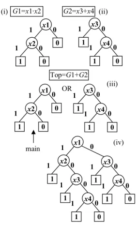
Figure 3. Example FT converted to BDD, using the ite technique

Consider the example in Figure 3. The ordering x1 <

x2 < x3 < x4 < x5 represents a simple top-down left-right Top G2 x2 x4 G1 x2 x3 x1 x1 1 0 1 0 x2 1 x3 1 0 1 0 0 x4 1 0 0 Top G2 x2 x5 x1 G1 x2 x3 x4 x1 1 0 1 0 x2 1 x3 1 0 1 0 x5 1 0 0 0 x4 1 0 0 x1 1 0 1 0 x2 1 0 terminal node root vertex 0 branch 1 branch non-terminal node

traversal of the fault tree. The application of the rules give the expressions for gates G1, G2 and Top:

G1 = x2 + x3 + x4

= ite(x2,1,0) + ite(x3,1,0) + ite(x4,1,0) = ite(x2,1,ite(x3,1,0)) + ite(x4,1,0) = ite(x2,1,ite(x3,1,ite(x4,1,0))) G2 = x2 + x5

= ite(x2,1,0) + ite(x5,1,0) = ite(x2,1,ite(x5,1,0)) Top = x1·G1·G2

= ite(x1,1,0)·

ite(x2,1,ite(x3,1,ite(x4,1,0)))·G2 = ite(x1,ite(x2,1,ite(x3,1,ite(x4,1,0))),0)·

ite(x2,1,ite(x5,1,0))

= ite(x1,ite(x2,1,ite(x3,f1,ite(x4,f1,0))),0) where

f1= ite(x5,1,0)

The resulting BDD is shown in Figure 3 and is an ordered BDD, where traversing the BDD along any path from the root vertex will encounter the nodes in the order specified. For example, the variables in the path x1,x2 appear according to the established ordering. Using this approach the variable ordering is retained throughout the BDD because every step of the connection is performed according to the ordering of the elements.

The method automatically uses sub-node sharing storing each ite structure in the memory only once and reusing calculated ite structures further in the process.

4. Component connection methods

4.1. Basic approach (approach 2)

The basic method of the second approach, the component connection method, is presented in [4]. The method starts by considering those gates which have only basic events as inputs. These gates are expressed as a BDD structure, which is known to represent “AND” or “OR” gate types. It then ascends the fault tree structure considering any gate whose inputs are already expressed as BDDs. It builds a BDD for an “AND” gate or an “OR” gate utilising simple rules of connection. Initially BDDs for fault trees are constructed without considering the repetition along the BDD paths of basic events in the fault tree. The resulting BDD then undergoes a simplification procedure. The connection and simplification rules with some alternative strategies are presented in this section. The ordering of basic events is not necessary for this approach, since the connection process can be applied without following any fixed ordering scheme for the whole system. However, a selection scheme has to be specified which will define the way in which gate inputs,

either basic events or BDDs, are selected for the connection process.

The connection rules are:

1. If a gate is an “AND” gate, the BDD nodes representing its inputs are connected to each other through the 1-branches of the nodes. If a gate is an “OR” gate, the BDD nodes are connected through the 0-branches (see Figure 4(i) and (ii)).

2. While merging two BDDs, representing two inputs of a parent gate, one of them is set to be the main BDD, according to the rule of selection. Then, if two BDDs are inputs to an “AND” gate, the secondary BDD is connected to every terminal 1-node of the main BDD or if two BDDs are inputs to an “OR” gate, the secondary BDD is connected to every terminal 0-node of the main BDD (see Figure 4(iii) and (iv)).

Figure 4. Example of connection rules

BDDs constructed in this way can feature more than one node representing the same variable on its paths. In order to avoid contradictory states of the repeated events in the BDD each path featuring a repeated variable can be simplified using the following rule:

The first occurrence of the event in the path specifies the state of the repeated variable. The node, that represents the second occurrence of the event, then needs to be replaced by the events below it on either its 1 or 0

0 x1 0 1 x2 0 0 1 1 G1=x1·x2 0 0 x3 1 1 x4 0 1 1 0 x1 0 1 x2 0 0 1 1 0 0 x3 1 1 x4 0 1 1 main OR 0 x1 1 x2 0 1 1 0 0 x3 1 1 x4 0 1 1 0 0 x3 1 1 x4 0 1 1 G2=x3+x4 Top=G1+G2 (i) (ii) (iii) (iv)

branch, depending on the component state specified by its first occurrence in the path. For example, if the path passes through the 1-branch of a node, the second appearance of that event should be replaced by the BDD structure below the 1-branch of this second node. If the path passes through the first variable occurrence on its 0-branch, the second occurrence of the variable is replaced by the BDD structure on its 0-branch.

A second rule to simplify the BDD can also be applied: If the BDD structures below the 1 and 0 branches of any node are the same, this node is irrelevant and needs to be replaced by the structure below either one of the branches. In other words, if the state of the system does not depend on the occurrence of the basic event, the insignificant node must be removed.

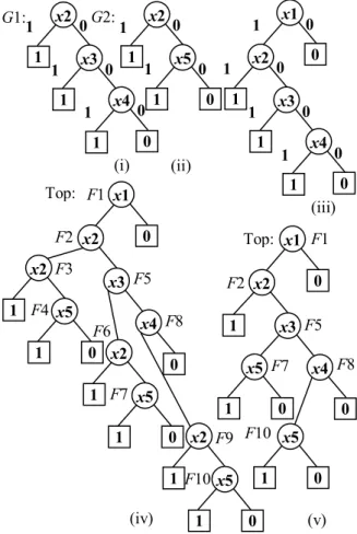
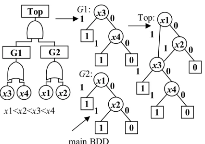
To demonstrate this approach it has been applied to the fault tree illustrated in Figure 3 resulting in the BDD in Figure 5. In this example the fault tree is traversed in the bottom-up manner. When constructing any gate BDD the variables are considered in a left-right variable ordering for every gate in a fault tree. The left-most BDD input for any gate is set to be the main BDD to which the others are joined.

The connection process starts constructing two BDDs for gates G1 and G2, shown in Figure 5(i) and Figure 5(ii) respectively. Since gates G1 and G2 are “OR” gates, the resulting BDDs are “OR” chains.

Then the top event, which is an “AND” gate is considered. The left-most BDD, basic event x1, is selected as the main BDD. Then the two BDDs from Figure 5(i) and 5(ii) are connected one by one to the 1 branch of the main BDD. The first connection results in the BDD in Figure 5(iii). The BDD after the last connection is presented in Figure 5(iv), where all left branches are 1 branches and right branches are 0 branches.

Finally, the simplification rules are applied. There is only one repeated event, x2, and its repetitions need to be removed from three current paths. In the first path F1-F

2-F3-F4 node F3 is replaced by the terminal 1-node, since this path traverses the 1-branch of node F2, the first occurrence of the repeated event. In the second path F

1-F2-F5-F6-F7 the repeated event x2 is removed, replacing node F6 by node F7. In the same way node F9 is replaced by node F10 in the third path F1-F2-F5-F8-F9-F10. The final BDD is shown in Figure 5(v).

In this example the basic events were connected according to the order that they appear in the list of gate inputs. However, it is possible to apply a defined ordering scheme for the nodes which will be used during the construction method. There is a number of structural or weighted ordering schemes [5], that can be applied. The chosen ordering schemes can affect the efficiency of the conversion process.

BDDs were selected according to the order that gate inputs are listed, i.e. the BDD, presenting the left-most gate, is set to be the main BDD. Other selection schemes can be used which can result in a smaller BDD and/or in a shorter processing time. BDDs can be ordered according to the position of their root vertex in an ordering scheme defined for the basic events or according to the smallest number of available branches where connections will be made. The efficiency of different strategies can be analysed comparing the number of nodes in the final BDD and the processing time.

Figure 5. Example FT converted to BDD, using the component connection method

The component connection process does not require the variable ordering applying the described connection rules. Therefore, even if the variable ordering is set from the start, i.e. for the conversion of gates including basic event inputs only, it is not retained when merging two BDDs. The resulting BDD of the component connection method is not an ordered BDD as achieved using the conventional approach. It does however retain the disjoint path property.

The basic component connection method does not use the sub-node sharing and it can lead to inefficient memory

0 x2 1 1 x3 0 0 x4 0 1 1 1 1 G1: (i) 0 x2 1 1 x5 0 0 1 1 G2: (ii) x1 0 x2 x3 x4 0 x5 0 1 1 x5 0 1 Top: F1 F2 F5 F7 F8 F10 (v) x1 0 x2 x3 x4 0 x2 1 x5 0 1 x2 1 _x5 0 1 x2 1 x5 0 1 Top: F1 F2 F3 F4 F5 F6 F7 F8 F9 F10 (iv) 0 x2 1 1 x3 0 0 x4 0 1 1 1 1 (iii) 0 x1 0 1

usage. For example, in Figure 5(v) there are two identical nodes F7 and F10, which could be shared in the BDD obtained using the ite technique (Figure 3). Therefore, an extension to the component connection method is made by introducing a form of sub-node sharing.

4.2. Sub-node sharing (approach 3)

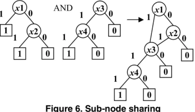
Sub-node sharing adds a significant contribution to the efficiency of the conventional BDD construction approach. It can be also implemented in the component connection method during the connection of two BDDs, for example, merging two inputs for an “AND” gate, as it is illustrated in Figure 6.

Figure 6. Sub-node sharing

In this example the left BDD is set to be the main BDD. It has two available connection points, i.e. two terminal 1-vertices, that can share the same copy of the second BDD. This connection is always suitable if the BDDs contain no repeated events in the fault tree.

The conversion method starts by applying the first connection rule, presented in the previous section, considering those gates which have only basic events as inputs. Then the process continues ascending the fault tree structure. The second rule is applied while merging the BDDs representing gate inputs. Applying the sub-node sharing the secondary BDD can be connected to all terminal nodes if while descending the BDD from the root vertex the same branches (1-branches or 0-branches) of repeated events were traversed. Otherwise, a new copy of the secondary BDD needs to be used.

The sub-node sharing rule is:

If paths to two terminal vertices (two terminal 1-nodes for BDDs being inputs to an AND gate and two terminal 0-nodes for BDDs being inputs to an OR gate) traverse the same branches of repeated events, the same copy of the second BDD can be connected to both of the two terminal nodes.

In the example from Figure 5, the BDD in 5(iii) is set to be the main BDD during the last connection of the two BDDs (Figure 5(ii), Figure 5(iii)). Since the BDDs represent two gate inputs to an AND gate the paths from the root vertex to the three terminal 1-nodes of the main BDD are investigated. There is only one repeated event

x2 in the fault tree. The first path passes the 1-branch of node x2, the second and the third paths pass the 0-branch of node x2. Since the second and the third paths pass the same branch of the repeated node the second and the third terminal nodes can be replaced by the same copy of the secondary BDD. The final BDD is shown in Figure 7(i) and 7(ii), after the connection and after the simplification processes respectively.

Figure 7. Application of sub-node sharing to the component connection method

The resulting BDD in Figure 7(ii) matches the one obtained using the ite technique, Figure 3.

Note. Applying the sub-node sharing all repeated events in the system must to be considered, not only those between the two BDDs under the current connection.

4.3. Hybrid approach (approach 4)

This approach is introduced to utilise the efficient parts of each algorithm presented. It is clear, that:

i) using the gate constructs for basic events and branches without repeated events BDDs can be immediately formulated without any of processing required by the ite method.

ii) the sub-node sharing feature of the ite method provides a more efficient representation of the logic function.

Therefore, a new algorithm has been created based on the effective features of each approach to obtain the best efficiency.

As was described before, using the component connection method does not require the variable ordering. However, since this new approach also uses the ite method a variable ordering needs to be introduced to the component connection method. This then produces ordered BDDs, which are used for the ite technique. 0 0 x1 1 1 x2 0 1 1 0 x3 0 1 x4 0 0 1 1 0 0 x1 1 x2 0 1 0 x3 0 1 x4 0 0 1 1 AND Top: F1 F2 F3 F4 F5 F8 x1 0 x2 x3 x4 0 x2 1 x5 0 1 x2 1 x5 0 1 F6 F7 (i) x1 1 0 1 0 x2 1 x3 1 0 1 0 x5 1 0 0 0 x4 1 0 Top: F1 F2 F5 F7 F8 (ii)

First of all, a variable ordering needs to be established which will be used when applying the rules of both methods. Then the building of BDDs for gates containing event inputs only starts, where events are put in a chain according to the type of the gate (component connection approach). This construction process can be applied regardless of the number of events into a gate without breaking them down into pairs, since the rules in the ite technique deal only with two ite structures at once. The variable ordering needs to be retained while putting basic events in a chain. The comparison of the component connection method and its application in the hybrid method is shown in Figure 8.

Figure 8. Comparison between the two methods while converting a gate with event

inputs only

For more complex parts, that do not contain any repeated events, the straightforward connection can be also applied. However, the variable ordering needs to be taken into the consideration, i.e. the merging of the two BDDs can be applied only if all the events of the main BDD are before the events of the secondary BDD in the variable ordering. This situation is shown in Figure 9.

While building the BDD for gates with repeated events, the ite technique rules are applied.

For example in Figure 3, BDDs for gates G1 and G2 are created placing its basic events in “OR” chains as it was shown in Figure 5(i) and (ii). Then the BDDs are merged applying the ite rules, given in equations 5 and 6.

Figure 9. Hybrid approach for the parts without repeated events

5. Comparison of the methods

The performance of the conversion methods will depend on the structure of the fault tree. An indication of any advantages can only be measured over a large range of problems. The four approaches discussed in this paper were investigated using a library of 12 fault trees. Their characteristics are shown in Table 1.

Table 1. Characteristics of example fault trees

Test FT Number of Gates Number of Basic Events Number of Repeated Events Number of Minimal Cut Sets 1 48 94 33 6391 2 51 53 2 764 3 52 47 8 122 4 46 64 12 423 5 48 114 64 66083 6 45 100 52 3344 7 46 84 25 1633 8 49 98 44 8113 9 48 72 14 493 10 38 58 15 898 11 54 110 56 200063 12 37 77 38 45505

The first column identifies the example fault tree, then the next three columns present indications of the complexity of the fault tree in terms of the number of gates, the number of basic events and the number of repeated events. The last column presents the number of minimal cut sets. Trying to achieve a consistent comparison of the four methods the variable ordering for 0 x1 1 1 x2 0 0 x3 0 1 1 1 1 G1: G1 x1 x3 x2 0 x1 1 1 x3 0 0 x2 0 1 1 1 1 G1: Component connection method Hybrid, x1<x2<x3 Top G2 x1 x2 G1 x3 x4 x1<x2<x3<x4 0 x1 1 1 x2 0 0 1 1 G2: 0 x3 1 1 x4 0 0 1 1 G1: main BDD 0 x1 1 x2 0 0 1 0 x3 1 1 x4 0 0 1 1 Top:

basic events was chosen not only for the conventional method but also for the component connection method, even though it is not needed. The modified top-down left-right approach for the ordering of basic events was applied [5].

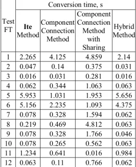
The measurements, that were chosen for the comparison of the four methods are: the number of nodes in the final BDD, the maximum number of lines in the storage array (representing the number of intermediate calculations performed), and the processing time. The results obtained by applying the four methods to the fault trees in the library are shown in Table 2, Table 3 and Table 4 respectively.

Table 2. Final BDD size of the four construction methods

Number of nodes in final BDD Test FT Ite Method Component Connection Method Component Connection Method with Sharing Hybrid Method 1 12470 189823 99046 12470 2 860 3153 2105 860 3 368 1114 899 368 4 1472 3876 2614 1472 5 18460 207800 81068 18460 6 16797 529729 20027 16797 7 1726 11306 5659 1726 8 1945 6980 2762 1945 9 1618 4085 2311 1618 10 1701 13324 11751 1701 11 8026 89466 13040 8026 12 1006 11729 2169 1006

Table 3. Number of intermediate calculations in the storage array of the four construction

methods

Number of lines in storage array Test FT Ite Method Component Connection Method Component Connection Method with Sharing Hybrid Method 1 12684 2084163 111880 12668 2 1138 59326 2129 1121 3 579 17752 1051 560 4 1773 359319 2614 1749 5 18639 452066 81933 18629 6 17149 1575967 20827 17134 7 1932 336782 6556 1916 8 2138 257947 2870 2130 9 1951 277230 2315 1930 10 1950 80371 11779 1931 11 8194 414932 13312 8191 12 1138 71507 2179 1129

Table 4. Processing time of the four construction methods Conversion time, s Test FT Ite Method Component Connection Method Component Connection Method with Sharing Hybrid Method 1 2.265 4.125 4.859 2.14 2 0.047 0.14 0.375 0.031 3 0.016 0.031 0.281 0.016 4 0.062 0.344 1.063 0.063 5 5.953 1.031 1.953 5.656 6 5.156 2.235 1.093 4.375 7 0.078 0.328 1.594 0.062 8 0.219 0.469 4.812 0.063 9 0.078 0.328 1.766 0.046 10 0.078 0.265 0.562 0.063 11 1.234 0.641 0.016 0.984 12 0.063 0.11 0.766 0.062

The first construction method (ite method) resulted in smaller BDDs and smaller number of lines in the storage array for all the example fault trees than the component connection method. The processing time was also shorter for almost all example fault trees, except three cases, (5), (6) and (11). Results for the basic approach of the component connection method were presented in [6].

Using the component connection approach with the sub-node sharing all the BDDs generated were smaller than using the basic component connection method, but the processing time increased, except examples (6) and (9), due to an extra time taken to identify parts in the BDD suitable for the sub-node sharing.

The hybrid method resulted in BDDs with the same number of nodes than the conventional approach. However, it gave slightly better results in terms of the two other measurements, the number of lines in the storage array and the computational time. This was due to the capability to obtain the BDDs for gates with event inputs only in a more efficient way, i.e. inputs of a gate were placed in a chain straightforwardly without the need to do it one by one. Also, more complex parts of the fault tree

without repeated events were converted to the BDD using the rules of the component connection method. In summary, using the hybrid method resulted in the same size of the final BDD as applying the conventional approach, but a better efficiency was achieved, since the computational time was shorter and the maximum number of lines in the storage array was smaller. Therefore, the hybrid method can be used as an efficient alternative technique for converting fault trees to BDDs.

6.Conclusions

This paper presents four approaches for the conversion of fault trees to BDDs. The first method is Rauzy’s ite method, the second is the basic component connection method. The third approach is an advanced form of the component connection method. A hybrid method which utilises the more efficient features of two basic methods is also presented. Test fault trees have been used and the results for the four methods compared. Conversion time, number of nodes in the final BDD and number of lines in the storage array were used as efficiency measures while working on all the methods. It is shown that as a general fault tree to BDD conversion technique the method proposed by Rauzy performs well. The component

connection method does not compete with Rauzy’s method very well even if the sub-node is incorporated. However, the hybrid method, as a mixture of two approaches, can provide a good alternative technique for conversion of fault trees to BDDs.

7. References

[1] A. Rauzy, “New Algorithms for Fault Tree Analysis,” Reliability Engineering and System Safety, no. 40, 1993, pp. 203-21.

[2] W.E. Vesely, “A Time Dependent Methodology for Fault Tree Evaluation”, Nuclear Design and Engineering, no. 13, 1970, pp. 337-360.

[3] R.M. Sinnamon, J.D. Andrews, “Improved Accuracy in Quantitative Fault Tree Analysis”, Quality and Reliability Engineering International, no. 13, 1997, pp. 285-292.

[4] Y.S. Way, D.Y. Hsia, “A simple component-connection method for building binary decision diagrams encoding a fault tree”, Reliability Engineering and System Safety, no. 70, 2000, pp. 59-70.

[5] K.A. Reay, “Efficient Fault Tree Analysis Using Binary Decision Diagrams”, Doctoral Thesis, Loughborough University, 2002.

[6] J.D. Andrews, R. Remenyte, ''Fault Tree Conversion to Binary Decision Diagrams'' , Proceedings of the 23rd ISSC , San Diego, USA, August 2005, ISBN 0-9721385-5-2 , [CD-ROM].