Fast Feature Pyramids for Object Detection

Fast Feature Pyramids for Object Detection

Piotr Doll ´ar, Ron Appel, Serge Belongie, and Pietro Perona

Abstract—Multi-resolution image features may be approximated via extrapolation from nearby scales, rather than being computed explicitly. This fundamental insight allows us to design object detection algorithms that are as accurate, and considerably faster, than the state-of-the-art. The computational bottleneck of many modern detectors is the computation of features at every scale of a finely-sampled image pyramid. Our key insight is that one may compute finely finely-sampled feature pyramids at a fraction of the cost, without sacrificing performance: for a broad family of features we find that features computed at octave-spaced scale intervals are sufficient to approximate features on a finely-sampled pyramid. Extrapolation is inexpensive as compared to direct feature computation. As a result, our approximation yields considerable speedups with negligible loss in detection accuracy. We modify three diverse visual recognition systems to use fast feature pyramids and show results on both pedestrian detection (measured on the Caltech, INRIA, TUD-Brussels and ETH datasets) and general object detection (measured on the PASCAL VOC). The approach is general and is widely applicable to vision algorithms requiring fine-grained multi-scale analysis. Our approximation is valid for images with broad spectra (most natural images) and fails for images with narrow band-pass spectra (e.g. periodic textures).

Index Terms—visual features, object detection, image pyramids, pedestrian detection, natural image statistics, real-time systems

F

1

I

NTRODUCTION

Multi-resolution multi-orientation decompositions are one of the foundational techniques of image analysis. The idea of analyzing image structure separately at every scale and orientation originated from a number of sources: measurements of the physiology of mammalian visual systems [1], [2], [3], principled reasoning about the statistics and coding of visual information [4], [5], [6], [7] (Gabors, DOGs, and jets), harmonic analysis [8], [9] (wavelets), and signal processing [9], [10] (multirate filtering). Such representations have proven effective for visual processing tasks such as denoising [11], image enhancement [12], texture analysis [13], stereoscopic cor-respondence [14], motion flow [15], [16], attention [17], boundary detection [18] and recognition [19], [20], [21].

It has become clear that such representations are best at extracting visual information when they are over-complete, i.e. when one oversamples scale, orientation and other kernel properties. This was suggested by the architecture of the primate visual system [22], where striate cortical cells (roughly equivalent to a wavelet ex-pansion of an image) outnumber retinal ganglion cells (a representation close to image pixels) by a factor ranging from 102 _{to 10}3_{. Empirical studies in computer vision} provide increasing evidence in favor of overcomplete representations [23], [24], [25], [21], [26]. Most likely the robustness of these representations with respect to changes in viewpoint, lighting, and image deformations is a contributing factor to their superior performance.

• P. Doll´ar is with the Interactive Visual Media Group at Microsoft Research, Redmond.

• R. Appel and P. Perona are with the Department of Electrical Engineering, California Institute of Technology, Pasadena.

• S. Belongie is with Cornell NYC Tech and the Cornell Computer Science Department.

To understand the value of richer representations, it is instructive to examine the reasons behind the breathtak-ing progress in visual category detection durbreathtak-ing the past ten years. Take, for instance, pedestrian detection. Since the groundbreaking work of Viola and Jones (VJ) [27], [28], false positive rates have decreased two orders of magnitude. At 80% detection rate on the INRIA pedes-trian dataset [21], VJ outputs over 10 false positives per image (FPPI), HOG [21] outputs ∼_{1 FPPI, and more} recent methods [29], [30] output well under 0.1 FPPI (data from [31], [32]). In comparing the different detec-tion schemes one notices the representadetec-tions at the front end are progressively enriched (e.g. more channels, finer scale sampling, enhanced normalization schemes); this has helped fuel the dramatic improvements in detection accuracy witnessed over the course of the last decade.

Unfortunately, improved detection accuracy has been accompanied by increased computational costs. The VJ detector ran at∼15 frames per second (fps) over a decade ago, on the other hand, most recent detectors require multiple seconds to process a single image as they com-pute richer image representations [31]. This has practical importance: in many applications of visual recognition, such as robotics, human computer interaction, automo-tive safety, and mobile devices, fast detection rates and low computational requirements are of the essence.

Thus, while increasing the redundancy of the rep-resentation offers improved detection and false-alarm rates, it is paid for by increased computational costs. Is this a necessary trade-off? In this work we offer the hoped-for but surprising answer: no.

We demonstrate how to compute richer representa-tions without paying a large computational price. How is this possible? The key insight is that natural images have fractal statistics [7], [33], [34] that we can exploit to reliably predict image structure across scales. Our

anal-ysis and experiments show that this makes it possible to inexpensively estimate features at a dense set of scales by extrapolating computations carried out expensively, but infrequently, at a coarsely sampled set of scales.

Our insight leads to considerably decreased run-times for state-of-the-art object detectors that rely on rich repre-sentations, including histograms of gradients [21], with negligible impact on their detection rates. We demon-strate the effectiveness of our proposed fast feature pyramids with three distinct detection frameworks in-cluding integral channel features [29], aggregate channel features (a novel variant of integral channel features), and deformable part models [35]. We show results for both pedestrian detection (measured on the Caltech [31], INRIA [21], TUD-Brussels [36] and ETH [37] datasets) and general object detection (measured on the PASCAL VOC [38]). Demonstrated speedups are significant and impact on accuracy is relatively minor.

Building on our work on fast feature pyramids (first presented in [39]), a number of systems show state-of-the-art accuracy while running at frame rate on640×480

images. Aggregate channel features, described in this pa-per, operate at over 30 fps while achieving top results on pedestrian detection. Crosstalk cascades [40] use fast fea-ture pyramids and couple detector evaluations of nearby windows to achieve speeds of 35-65 fps. Benenson et al. [30] implemented fast feature pyramids on a GPU, and with additional innovations achieved detection rates of over 100 fps. In this work we examine and analyze feature scaling and its effect on object detection in far more detail than in our previous work [39].

The rest of this paper is organized as follows. We review related work in §2. In §3 we show that it is possible to create high fidelity approximations of multi-scale gradient histograms using gradients computed at a single scale. In§4we generalize this finding to a broad family of feature types. We describe our efficient scheme for computing finely sampled feature pyramids in §5. In §6 we show applications of fast feature pyramids to object detection, resulting in considerable speedups with minor loss in accuracy. We conclude in§7.

2

R

ELATED

W

ORK

Significant research has been devoted to scale space theory [41], including real time implementations of oc-tave and half-ococ-tave image pyramids [42], [43]. Sparse image pyramids often suffice for certain approximations, e.g. [42] shows how to recover a disk’s characteristic scale using half-octave pyramids. Although only loosely related, these ideas provide the intuition that finely sampled feature pyramids can perhaps be approximated. Fast object detection has been of considerable interest in the community. Notable recent efforts for increasing detection speed include work by Felzenszwalb et al. [44] and Pedersoli et al. [45] on cascaded and coarse-to-fine deformable part models, respectively, Lampert et al.’s [46] application of branch and bound search for

detection, and Doll´ar et al.’s work on crosstalk cascades [40]. Cascades [27], [47], [48], [49], [50], coarse-to-fine search [51], distance transforms [52], etc., all focus on op-timizing classification speed given precomputed image features. Our work focuses on fast feature pyramid con-struction and is thus complementary to such approaches. An effective framework for object detection is the sliding window paradigm [53], [27]. Top performing methods on pedestrian detection [31] and the PASCAL VOC [38] are based on sliding windows over multiscale feature pyramids [21], [29], [35]; fast feature pyramids are well suited for such sliding window detectors. Al-ternative detection paradigms have been proposed [54], [55], [56], [57], [58], [59]. Although a full review is outside the scope of this work, the approximations we propose could potentially be applicable to such schemes as well. As mentioned, a number of state-of-the-art detectors have recently been introduced that exploit our fast fea-ture pyramid construction to operate at frame rate in-cluding [40] and [30]. Alternatively, parallel implementa-tion using GPUs [60], [61], [62] can achieve fast detecimplementa-tion while using rich representations but at the cost of added complexity and hardware requirements. Zhu et al. [63] proposed fast computation of gradient histograms using integral histograms [64]; the proposed system was real time for single-scale detection only. In scenarios such as automotive applications, real time systems have also been demonstrated [65], [66]. The insights outlined in this paper allow for real time multiscale detection in general, unconstrained settings.

3

M

ULTISCALE

G

RADIENT

H

ISTOGRAMS We begin by exploring a simple question: given image gradients computed at one scale, is it possible to approximate gradient histograms at a nearby scale solely from the computed gradients?If so, then we can avoid computing gradients over a finely sampled image pyramid. Intuitively, one would expect this to be possible, as significant image structure is preserved when an image is resampled. We begin with an in-depth look at a simple form of gradient histograms and develop a more general theory in§4.

A gradient histogram measures the distribution of the gradient angles within an image. Let I(x, y) denote an m ×n discrete signal, and ∂I/∂x and ∂I/∂y denote the discrete derivatives of I (typically 1D centered first differences are used). Gradient magnitude and orien-tation are defined by: M(i, j)2 = ∂I_∂x(i, j)2 + ∂I_∂y(i, j)2

and O(i, j) = arctan ∂I_∂y(i, j)/∂I_∂x(i, j)

. To compute the gradient histogram of an image, each pixel casts a vote, weighted by its gradient magnitude, for the bin corresponding to its gradient orientation. After the ori-entation O is quantized into Q bins so that O(i, j) ∈ {1, Q}, the qth bin of the histogram is defined by: hq = P

i,jM(i, j)1[O(i, j) =q], where 1 is the indicator func-tion. In the following everything that holds for global histograms also applies to local histograms (defined identically except for the range of the indicesiand j).

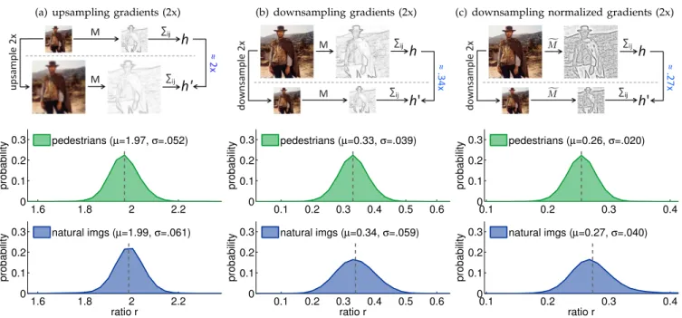
(a) upsampling gradients (2x) 1.6 1.8 2 2.2 0 0.1 0.2 0.3 ratio r probability pedestrians (µ=1.97, σ=.052) 1.6 1.8 2 2.2 0 0.1 0.2 0.3 ratio r probability natural imgs (µ=1.99, σ=.061) (b) downsampling gradients (2x) 0.1 0.2 0.3 0.4 0.5 0.6 0 0.1 0.2 0.3 ratio r probability pedestrians (µ=0.33, σ=.039) 0.1 0.2 0.3 0.4 0.5 0.6 0 0.1 0.2 0.3 ratio r probability natural imgs (µ=0.34, σ=.059)

(c) downsampling normalized gradients (2x)

0.1 0.2 0.3 0.4 0 0.1 0.2 0.3 ratio r probability pedestrians (µ=0.26, σ=.020) 0.1 0.2 0.3 0.4 0 0.1 0.2 0.3 ratio r probability natural imgs (µ=0.27, σ=.040)

Fig. 1. Behavior of gradient histograms in images resampled by a factor of two.(a) Upsampling gradients: Given imagesIand I0whereI0denotesIupsampled by two, and corresponding gradient magnitude imagesM andM0, the ratioΣM/ΣM0should be approximately2. The middle/bottom panels show the distribution of this ratio for gradients at fixed orientation over pedestrian/natural images. In both cases the mean µ ≈2, as expected, and the variance is relatively small.(b) Downsampling gradients: Given images I andI0 whereI0 denotesI downsampled by two, the ratioΣM/ΣM0 ≈ .34, not .5as might be expected from (a) as downsampling results in loss of high frequency content. (c) Downsampling normalized gradients: Givennormalized gradient magnitude imagesMfandMf0, the ratioΣM /f ΣMf0 ≈.27. Instead of trying to derive analytical expressions governing the scaling properties of various feature types under different resampling factors, in§4we describe a general law governing feature scaling.

3.1 Gradient Histograms in Upsampled Images Intuitively the information content of an upsampled image is similar to that of the original, lower-resolution image (upsampling does not create new structure). As-sume I is a continuous signal, and let I0 denote I upsampled by a factor of k: I0(x, y) ≡ I(x/k, y/k). Using the definition of a derivative, one can show that

∂I0

∂x(i, j) = 1 k

∂I

∂x(i/k, j/k), and likewise for ∂I0

∂y, which simply states the intuitive fact that the rate of change in the upsampled image isktimes slower the rate of change in the original image. While not exact, the above also holds approximately for interpolated discrete signals. Let M0(i, j) ≈ 1

kM(di/ke,dj/ke) denote the gradient magnitude in an upsampled discrete image. Then:

kn X i=1 km X j=1 M0(i, j)≈ kn X i=1 km X j=1 1 kM(di/ke,dj/ke) (1) =k2 n X i=1 m X j=1 1 kM(i, j) =k n X i=1 m X j=1 M(i, j)

Thus, the sum of gradient magnitudes in the original and upsampled image should be related by about a factor ofk. Angles should also be mostly preserved since

∂I0 ∂x(i, j) ∂I0 ∂y(i, j)≈ ∂I ∂x(i/k, j/k) ∂I

∂y(i/k, j/k). Therefore, according to the definition of gradient histograms, we expect the relationship between hq (computed over I) and h0q (computed over I0) to be: h0q ≈khq. This allows us to approximate gradient histograms in an upsampled image using gradients computed at the original scale.

Experiments: One may verify experimentally that in images of natural scenes, upsampled using bilinear in-terpolation, the approximation h0_q ≈ khq is reasonable. We use two sets of images for these experiments, one class specific and one class independent. First, we use the 1237 cropped pedestrian images from the INRIA pedestrians training dataset [21]. Each image is128×64

and contains a pedestrian approximately 96 pixels tall. The second image set contains128×64windows cropped at random positions from the1218images in the INRIA negative training set. We sample 5000 windows but exclude nearly uniform windows, i.e. those with average gradient magnitude under.01, resulting in 4280 images. We refer to the two sets as ‘pedestrian images’ and ‘natural images’, although the latter is biased toward scenes that may (but do not) contain pedestrians.

In order to measure the fidelity of this approximation, we define the ratio rq =h0q/hq and quantize orientation into Q = 6 bins. Figure 1(a) shows the distribution of rq for one bin on the 1237 pedestrian and 4280 natural images given an upsampling of k= 2(results for other bins were similar). In both cases the mean is µ≈ 2, as expected, and the variance is relatively small, meaning the approximation is unbiased and reasonable.

Thus, although individual gradients may change, gra-dient histograms in an upsampled and original image will be related by a multiplicative constant roughly equal to the scale change between them. We examine gradient histograms in downsampled images next.

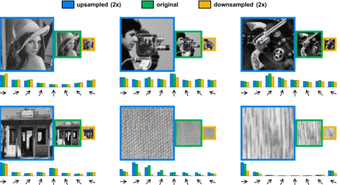
Fig. 2. Approximating gradient histograms in images resampled by a factor of two. For each image set, we take the original image (green border) and generate an upsampled (blue) and downsampled (orange) version. At each scale we compute a gradient histogram with 8 bins, multiplying each bin by.5and1/.34in the upsampled and downsampled histogram, respectively. Assuming the approximations from§3hold, the three normalized gradient histograms should be roughly equal (the blue, green, and orange bars should have the same height at each orientation). For the first four cases, the approximations are fairly accurate. In the last two cases, showing highly structured Brodatz textures with significant high frequency content, the downsampling approximation fails. The first four images are representative, the last two are carefully selected to demonstrate images with atypical statistics.

3.2 Gradient Histograms in Downsampled Images While the information content of an upsampled image is roughly the same as that of the original image, infor-mation is typically lost during downsampling. However, we find that the information loss is consistent and the re-sulting approximation takes on a similarly simple form. If I contains little high frequency energy, then the approximationh0q ≈khq derived in§3.1should apply. In general, however, downsampling results in loss of high frequency content which can lead to measured gradients undershooting the extrapolated gradients. Let I0 _now denote I downsampled by a factor of k. We expect that hq (computed over I) and h0q (computed over I0) will satisfyh0_q ≤hq/k. The question we seek to answer here is whether the information loss is consistent.

Experiments: As before, define rq = h0q/hq. In Fig-ure 1(b)we show the distribution ofrq for a single bin on the pedestrian and natural images given a down-sampling factor of k = 2. Observe that the information loss is consistent: rq is normally distributed around µ ≈ .34 < .5 for natural images (and similarly µ ≈.33

for pedestrians). This implies thath0_q ≈µhq could serve as a reasonable approximation for gradient histograms in images downsampled by k= 2.

In other words, similarly to upsampling, gradient histograms computed over original and half resolution images tend to differ by a multiplicative constant (al-though the constant is not the inverse of the sampling factor). In Figure 2 we show the quality of the above

approximations on example images. The agreement be-tween predictions and observations is accurate for typi-cal images (but fails for images with atypitypi-cal statistics). 3.3 Histograms of Normalized Gradients

Suppose we replaced the gradient magnitudeM by the normalized gradient magnitude Mfdefined as Mf(i, j) = M(i, j)/(M(i, j)+.005), whereM is the average gradient magnitude in each 11×11 image patch (computed by convolving M with an L1 normalized 11×11 triangle filter). Using the normalized gradientMfgives improved results in the context of object detection (see§6). Observe that we have now introduced an additional nonlinearity to the gradient computation; do the previous results for gradient histograms still hold if we useMfinstead ofM? In Figure 1(c) we plot the distribution of rq = h0q/hq for histograms of normalized gradients given a down-sampling factor of k = 2. As with the original gra-dient histograms, the distributions of rq are normally distributed and have similar means for pedestrian and natural images (µ ≈ .26 and µ ≈ .27, respectively). Observe, however, that the expected value of rq for normalized gradient histograms is quite different than for the original histograms (Figure1(b)).

Deriving analytical expressions governing the scaling properties of progressively more complex feature types would be difficult or even impossible. Instead, in§4 we describe a general law governing feature scaling.

4

S

TATISTICS OF

M

ULTISCALE

F

EATURES To understand more generally how features behave in resampled images, we turn to the study of natural image statistics [7], [33]. The analysis below provides a deep understanding of the behavior of multiscale features. The practical result is a simple yet powerful approach for predicting the behavior of gradients and other low-level features in resampled images without resorting to analytical derivations that may be difficult except under the simplest conditions.

We begin by defining a broad family of features. Let

Ω be any low-level shift invariant function that takes an image I and creates a new channel image C = Ω(I)

where a channel C is a per-pixel feature map such that output pixels in C are computed from corresponding patches of input pixels in I (thus preserving overall image layout). C may be downsampled relative to I and may contain multiple layers k. We define a feature fΩ(I) as a weighted sum of the channel C = Ω(I): fΩ(I) =P

ijkwijkC(i, j, k). Numerous local and global features can be written in this form including gradient histograms, linear filters, color statistics, and others [29]. Any such low-level shift invariantΩcan be used, making this representation quite general.

LetIsdenoteIat scales, where the dimensionshs×ws ofIsarestimes the dimensions ofI. Fors >1,Is(which denotes a higher resolution version ofI) typically differs from I upsampled by s, while for s < 1 an excellent approximation of Is can be obtained by downsampling I. Next, for simplicity we redefine fΩ(Is)as1:

fΩ(Is)≡ 1 hswsk X ijk Cs(i, j, k)whereCs= Ω(Is). (2)

In other words fΩ(Is) denotes the global mean of Cs computed over locations ij and layers k. Everything in the following derivations based on global means also holds for local means (e.g. local histograms).

Our goal is to understand how fΩ(Is) behaves as a function ofs for any choice of shift invariantΩ.

4.1 Power Law Governs Feature Scaling

Ruderman and Bialek [33], [67] explored how the statis-tics of natural images behave as a function of the scale at which an image ensemble was captured, i.e. the visual angle corresponding to a single pixel. Letφ(I)denote an arbitrary (scalar) image statistic andE[·]denote expecta-tion over an ensemble of natural images. Ruderman and Bialek made the fundamental discovery that the ratio of E[φ(Is1)]toE[φ(Is2)], computed over two ensembles of

natural images captured at scaless1ands2, respectively, depends only on the ratio of s1/s2 and is independent of the absolute scales s1 and s2 of the ensembles.

1. The definition offΩ(Is)in Eqn. (2) differs from our previous defi-nition in [39], wheref(I, s)denoted the channelsumafter resampling by2s_{. The new definition and notation allow for a cleaner derivation,}

and the exponential scaling law becomes a more intuitive power law.

Ruderman and Bialek’s findings imply that E[φ(Is)] follows a power law2_:

E[φ(Is1)]/E[φ(Is2)] = (s1/s2)

−λφ ₍₃₎

Every statisticφwill have its own correspondingλφ. In the context of our work, for any channel typeΩwe can use the scalar fΩ(I) in place of φ(I) and λΩ in place of λφ. While Eqn. (3) gives the behavior of fΩ w.r.t. to scale over an ensemble of images, we are interested in the behavior offΩ for asingleimage.

We observe that a single image can itself be considered an ensemble of image patches (smaller images). SinceΩ

is shift invariant, we can interpret fΩ(I) as computing the average of fΩ(Ik_{) over every patch I}k _{of I and} therefore Eqn. (3) can be applied directly for a single image. We formalize this below.

We can decompose an imageI intoKsmaller images I1. . . IK such that I = [I1· · ·IK]. Given that Ω must be shift invariant and ignoring boundary effects gives

Ω(I) = Ω([I1· · ·IK]) ≈[Ω(I1)· · ·Ω(IK)], and substitut-ing into Eqn. (2) yields fΩ(I) ≈ ΣfΩ(Ik)/K. However, we can consider I1_{· · ·I}K _{as a (small) image ensemble,} and fΩ(I) ≈ E[fΩ(Ik)] an expectation over that en-semble. Therefore, substitutingfΩ(Is1)≈E[fΩ(I

k s1)]and

fΩ(Is2)≈E[fΩ(I

k

s2)]into Eqn. (3) yields:

fΩ(Is1)/fΩ(Is2) = (s1/s2)

−λΩ_{+E , (4)}

where we useE to denote the deviation from the power law for a given image. Each channel typeΩhas its own correspondingλΩ, which we can determine empirically. In §4.2 we show that on average Eqn. (4) provides a remarkably good fit for multiple channel types and image sets (i.e. we can fit λΩ such thatE[E]≈0). Addi-tionally, experiments in§4.3indicate that the magnitude of deviation for individual images, E[E2_{], is reasonable} and increases only gradually as a function of s1/s2. 4.2 Estimatingλ

We perform a series of experiments to verify Eqn. (4) and estimateλΩfor numerous channel types Ω.

To estimateλΩ for a givenΩ, we first compute: µs= 1 N N X i=1 fΩ(Isi)/fΩ(I1i) (5) for N images Ii _{and multiple values of s < 1, where} I_si is obtained by downsampling I₁i = Ii. We use two image ensembles, one of N = 1237 pedestrian images and one of N = 4280 natural images (for details see

2. LetF(s) =E[φ(Is)]. We can rewrite the observation by saying there exists a functionRsuch thatF(s1)/F(s2) =R(s1/s2). Applying repeatedly givesF(s1)/F(1) =R(s1),F(1)/F(s2) = R(1/s2), and

F(s1)/F(s2) =R(s1/s2). ThereforeR(s1/s2) =R(s1)R(1/s2). Next, letR0(s) =R(es_{)and observe thatR}0_(s

1+s2) =R0(s1)R0(s2)since R(s1s2) =R(s1)R(s2). IfR0is also continuous and non-zero, then it must take the formR0(s) =e−λs_{for some constantλ[68]. This implies} R(s) =R0(ln(s)) =e−λln(s)_=s−λ_{. Therefore,E[φ(Is)]must follow} a power law (see also Eqn. (9) in [67]).

0 −0.5 −1 −1.5 −2 −2.5 −3 1 2 4 8 log2(scale) µ (ratio) pedestrians [0.037] natural imgs [0.018] best−fit: λ=0.406

(a) histograms of gradients

0 −0.5 −1 −1.5 −2 −2.5 −3 1 2 4 log2(scale) µ (ratio) pedestrians [0.026] natural imgs [0.006] best−fit: λ=0.101

(b) histograms of normalized gradients

0 −0.5 −1 −1.5 −2 −2.5 −3 1 2 4 8 16 log2(scale) µ (ratio) pedestrians [0.019] natural imgs [0.013] best−fit: λ=0.974

(c) difference of gaussians (DoG)

0 −0.5 −1 −1.5 −2 −2.5 −3 1 2 4 log2(scale) µ (ratio) pedestrians [0.000] natural imgs [0.000] best−fit: λ=0.000 (d) grayscale images 0 −0.5 −1 −1.5 −2 −2.5 −3 1 2 4 8 log2(scale) µ (ratio) pedestrians [0.044] natural imgs [0.025] best−fit: λ=0.358

(e) local standard deviation

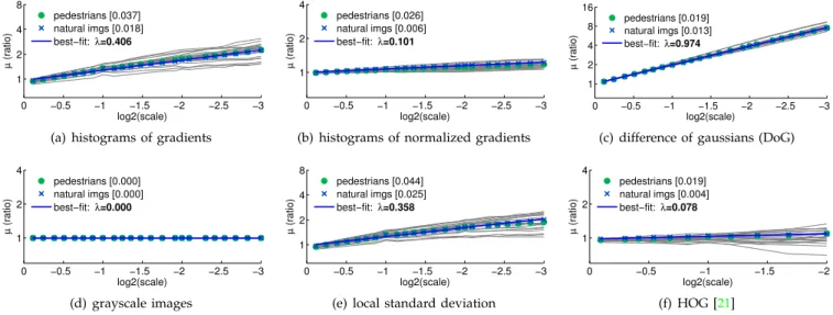
0 −0.5 −1 −1.5 −2 1 2 4 log2(scale) µ (ratio) pedestrians [0.019] natural imgs [0.004] best−fit: λ=0.078 (f) HOG [21] Fig. 3.Power Law Feature Scaling: For each of six channel types we plotµs = _N1 PfΩ(Isi)/fΩ(I1i)fors≈2

−1

8_{, . . . ,2}−248 _{on a} log-log plot for both pedestrian and natural image ensembles. Plots offΩ(Is1)/fΩ(Is2)for 20 randomly selected pedestrian images are shown as faint gray lines. Additionally the best-fit line toµs for the natural images is shown. The resultingλand expected error|E[E]|are given in the plot legends. In all cases theµsfollow a power law as predicted by Eqn. (4) and are nearly identical for both pedestrian and natural images, showing the estimate of λis robust and generally applicable. The tested channels are:

(a)histograms of gradients described in§3;(b)histograms of normalized gradients described in§3.3;(c)a difference of gaussian (DoG) filter (with inner and outerσof.71and1.14, respectively);(d)grayscale images (withλ= 0as expected);(e)pixel standard deviation computed over local5×5neighborhoodsC(i, j) =p

E[I(i, j)2_{]−E[I(i, j)];(f)HOG [21] with4×4spatial bins (results} were averaged over HOG’s 36 channels). Code for generating such plots is available (see chnsScaling.m in Piotr’s Toolbox).

§3.1). According to Eqn. (4),µs=s−λΩ+E[E]. Our goal is to fitλΩaccordingly and verify the fidelity of Eqn. (4) for various channel typesΩ(i.e. verify that E[E]≈0).

For each Ω, we measure µs according to Eqn. (5) across three octaves with eight scales per octave for a total of 24 measurements at s = 2−18, . . . ,2−248. Since

image dimensions are rounded to the nearest integer, we compute and use s0 = phsws/hw, where h×w and hs ×ws are the dimensions of the original and downsampled images, respectively.

In Figure 3 we plot µs versus s0 using a log-log plot for six channel types for both the pedestrian and natural images3_{. In all cases µ}

s follows a power law with all measurements falling along a line on the log-log plots, as predicted. However, close inspection showsµs does not start exactly at 1 as expected: downsampling introduces a minor amount of blur even for small downsampling factors. We thus expectµsto have the formµs=aΩs−λΩ, with aΩ6= 1as an artifact of the interpolation. Note that aΩ is only necessary for estimating λΩ from downsam-pled images and is not used subsequently. To estimate aΩ and λΩ, we use a least squares fit of log₂(µs0) =

a0_Ω−λΩlog₂(s0)to the24measurements computed over natural images (and set aΩ = 2a0_{Ω). Resulting estimates} of λΩare given in plot legends in Figure3.

There is strong agreement between the resulting best-fit lines and the observations. In legend brackets in Figure3we report expected error|E[E]|=|µs−aΩs−λΩ|

3. Figure3generalizes the results shown in Figure1. However, by switching from channel sums to channel means,µ1/2 in Figures3(a) and3(b)is4×larger thanµin Figures1(b)and1(c), respectively.

for both natural and pedestrian images averaged over s (using aΩ and λΩ estimated using natural images). For basic gradient histograms |E[E]| = .018 for natural images and|E[E]|=.037 for pedestrian images. Indeed, for every channel type Eqn. (4) is an excellent fit to the observationsµs for both image ensembles.

The derivation of Eqn. (4) depends on the distribution of image statistics being stationary with respect to scale; that this holds for all channel types tested, and with nearly an identical constant for both pedestrian and natural images, shows the estimate ofλΩ is robust and generally applicable.

4.3 Deviation for Individual Images

In §4.2 we verified that Eqn. (4) holds for an ensemble of images; we now examine the magnitude of deviation from the power law forindividual images. We study the effect this has in the context of object detection in§6.

Plots offΩ(Is1)/fΩ(Is2)for randomly selected images

are shown as faint gray lines in Figure3. The individual curves are relatively smooth and diverge only somewhat from the best-fit line. We quantify their deviation by defining σs analogously toµsin Eqn. (5):

σs=stdev[fΩ(Isi)/fΩ(I i

1)] =stdev[E], (6) where ‘stdev’ denotes the sample standard deviation (computed overN images) andE is the error associated with each image and scaling factor as defined in Eqn. (4). In§4.2we confirmed that E[E] ≈0, our goal now is to understand howσs=stdev[E]≈

p

0 −0.5 −1 −1.5 −2 −2.5 −3 0 0.2 0.4 0.6 0.8 1 log2(scale) σ (ratio) pedestrians [0.11] natural imgs [0.16]

(a) histograms of gradients

0 −0.5 −1 −1.5 −2 −2.5 −3 0 0.2 0.4 0.6 0.8 1 log2(scale) σ (ratio) pedestrians [0.03] natural imgs [0.05]

(b) histograms of normalized gradients

0 −0.5 −1 −1.5 −2 −2.5 −3 0 0.2 0.4 0.6 0.8 1 log2(scale) σ (ratio) pedestrians [0.03] natural imgs [0.03]

(c) difference of gaussians (DoG)

0 −0.5 −1 −1.5 −2 −2.5 −3 0 0.2 0.4 0.6 0.8 1 log2(scale) σ (ratio) pedestrians [0.00] natural imgs [0.00] (d) grayscale images 0 −0.5 −1 −1.5 −2 −2.5 −3 0 0.2 0.4 0.6 0.8 1 log2(scale) σ (ratio) pedestrians [0.10] natural imgs [0.16]

(e) local standard deviation

0 −0.5 −1 −1.5 −2 0 0.2 0.4 0.6 0.8 1 log2(scale) σ (ratio) pedestrians [0.07] natural imgs [0.07] (f) HOG [21]

Fig. 4. Power Law Deviation for Individual Images: For each of the six channel types described in Figure3we plotσsversuss whereσs=

p

E[E2_{]andEis the deviation from the power law for a single image as defined in Eqn. (4). In brackets we reportσ} 1/2 for both natural and pedestrian images.σsincreases gradually as a function ofs, meaning that not only does Eqn. (4) hold for an

ensembleof images but also the deviation from the power law forindividualimages is low for smalls.

In Figure4 we plotσs as a function ofsfor the same channels as in Figure 3. In legend brackets we reportσs for s = 1

2 for both natural and pedestrian images; for all channels studied σ1/2 < .2. In all casesσs increases gradually with increasing s and the deviation is low for small s. The expected magnitude of E varies across channels, for example histograms of normalized gradi-ents (Figure4(b)) have lowerσsthan their unnormalized counterparts (Figure 4(a)). The trivial grayscale channel (Figure4(d)) hasσs= 0as the approximation is exact.

Observe that often σs is greater for natural images than for pedestrian images. Many of the natural images contain relatively little structure (e.g. a patch of sky), for such imagesfΩ(I)is small for certainΩ(e.g. simple gradient histograms) resulting in more variance in the ratio in Eqn. (4). For HOG channels (Figure4(f)), which have additional normalization, this effect is minimized. 4.4 Miscellanea

We conclude this section with additional observations. Interpolation Method:Varying the interpolation algo-rithm for image resampling does not have a major effect. In Figure 5(a), we plot µ1/2 and σ1/2 for normalized gradient histograms computed using nearest neighbor, bilinear, and bicubic interpolation. In all three cases both µ1/2and σ1/2 remain essentially unchanged.

Window Size: All preceding experiments were per-formed on128×64windows. In Figure5(b)we plot the effect of varying the window size. While µ1/2 remains relatively constant, σ1/2 increases with decreasing win-dow size (see also the derivation of Eqn. (4)).

Upsampling: The power law can predict features in higher resolution images but not upsampled images. In practice, though, we want to predict features in higher resolution as opposed to (smooth) upsampled images.

(a) interpolation algorithm (b) window size

Fig. 5. Effect of the interpolation algorithm and window size on channel scaling.We plot µ1/2 (bar height) and σ1/2 (error bars) for normalized gradient histograms (see§3.3) .(a)Varying the interpolation algorithm for resampling does not have a major effect on eitherµ1/2orσ1/2.(b)Decreasing window size leaves µ1/2relatively unchanged but results in increasingσ1/2.

Robust Estimation: In preceding derivations, when computingfΩ(Is1)/fΩ(Is2)we assumed thatfΩ(Is2)6= 0.

For theΩ’s considered this was the case after windows of near uniform intensity were excluded (see§3.1). Alter-natively, we have found that excludingIwithfΩ(I)≈0

when estimatingλresults in more robust estimates. Sparse Channels: For sparse channels where fre-quentlyfΩ(I)≈0, e.g., the output of a sliding-window object detector, σ will be large. Such channels may not be good candidates for the power law approximation.

One-Shot Estimates: We can estimateλas described in §4.2using asingle imagein place of an ensemble (N = 1). Such estimates are noisy but not entirely unreasonable; e.g., on normalized gradient histograms (withλ≈.101) the mean of 4280 single image estimates ofλif.096and the standard deviation of the estimates is.073.

Scale Range: We expect the power law to break down at extreme scales not typically encountered under natu-ral viewing conditions (e.g. under high magnification).

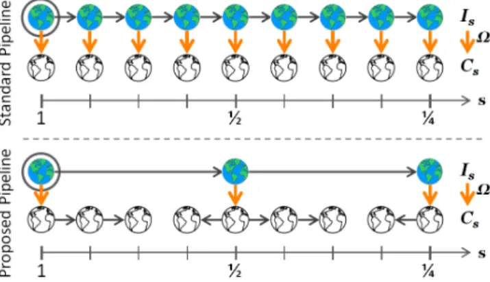
Fig. 6. Feature channel scaling. Suppose we have computed C = Ω(I); can we predictCs = Ω(Is)at a new scales?Top: the standard approach is to computeCs= Ω(R(I, s)), ignoring the information contained inC= Ω(I).Bottom: instead, based on the power law introduced in§4, we propose to approximate Cs by R(C, s) ·s−λΩ. This approach is simple, general, and accurate, and allows for fast feature pyramid construction.

5

F

AST

F

EATURE

P

YRAMIDS

We introduce a novel, efficient scheme for computing feature pyramids. First, in §5.1we outline an approach for scaling feature channels. Next, in §5.2 we show its application to constructing feature pyramids efficiently and we analyze computational complexity in §5.3. 5.1 Feature Channel Scaling

We propose an extension of the power law governing feature scaling introduced in §4 that applies directly to channel images. As before, let Is denote I captured at scale s and R(I, s) denote I resampled by s. Suppose we have computedC= Ω(I); can we predict the channel image Cs= Ω(Is)at a new scalesusing only C?

The standard approach is to computeCs= Ω(R(I, s)), ignoring the information contained inC= Ω(I). Instead, we propose the following approximation:

Cs≈R(C, s)·s−λΩ (7) A visual demonstration of Eqn. (7) is shown in Figure6. Eqn. (7) follows from Eqn. (4). Setting s1=s,s2= 1, and rearranging Eqn. (4) givesfΩ(Is)≈fΩ(I)s−λΩ. This relation must hold not only for the original images but also for any pair of corresponding windows ws and w in Is andI, respectively. Expanding yields:

fΩ(Iws s ) ≈ fΩ(Iw)s−λΩ 1 |ws| X i,j∈ws Cs(i, j) ≈ 1 |w| X i,j∈w C(i, j)s−λΩ Cs ≈ R(C, s)s−λΩ

The final line follows because if for all corresponding windowsP

wsC

0_{/|ws| ≈}P

wC/|w|, thenC

0_{≈R(C, s).} On aper-pixel basis, the approximation ofCsin Eqn. (7) may be quite noisy. The standard deviationσsof the ratio fΩ(Iws

s )/fΩ(Iw) depends on the size of the window w: σs increases asw decreases (see Figure 5(b)). Therefore, the accuracy of the approximation for Cs will improve if information is aggregated over multiple pixels of Cs.

Fig. 7. Fast Feature Pyramids. Color and grayscale icons represent images and channels; horizontal and vertical arrows denote computation ofRandΩ.Top: The standard pipeline for constructing a feature pyramid requires computingIs=R(I, s) followed by Cs = Ω(Is) for every s. This is costly. Bottom: We propose computingIs = R(I, s)and Cs = Ω(Is)for only a sparse set of s (once per octave). Then, at intermediate scales Cs is computed using the approximation in Eqn. (7): Cs ≈ R(Cs0, s/s0)(s/s0)−λΩ wheres0 is the nearest scale for which we have Cs0 = Ω(I_s0). In the proposed scheme, the number of computations ofRis constant while (more expensive) computations ofΩare reduced considerably.

A simple strategy for aggregating over multiple pix-els and thus improving robustness is to downsample and/or smooth Cs relative to Is (each pixel in the resulting channel will be a weighted sum of pixels in the original full resolution channel). DownsamplingCsalso allows for faster pyramid construction (we return to this in §5.2). For object detection, we typically downsample channels by4×to 8×(e.g. HOG [21] uses8×8 bins). 5.2 Fast Feature Pyramids

A feature pyramid is a multi-scale representation of an image I where channels Cs = Ω(Is) are computed at every scale s. Scales are sampled evenly in log-space, starting ats= 1, with typically 4 to 12 scales per octave (an octave is the interval between one scale and another with half or double its value). The standard approach to constructing a feature pyramid is to compute Cs =

Ω(R(I, s))for every s, see Figure7 (top).

The approximation in Eqn. (7) suggests a straightfor-ward method for efficient feature pyramid construction. We begin by computingCs= Ω(R(I, s))at just one scale per octave (s ∈ {1,1₂,1₄, . . .}). At intermediate scales, Csis computed using Cs≈R(Cs0, s/s0)(s/s0)−λΩ where

s0 ∈ {1,1₂,1₄, . . .} is the nearest scale for which we have Cs0 = Ω(I_s0), see Figure7 (bottom).

Computing Cs = Ω(R(I, s)) at one scale per octave provides a good tradeoff between speed and accuracy. The cost of evaluatingΩis within 33% of computingΩ(I)

at the original scale (see§5.3) and channels do not need to be approximated beyond half an octave (keeping error low, see§4.3). While the number of evaluations of R is constant (evaluations ofR(I, s)are replaced byR(C, s)), if eachCsis downsampled relative toIsas described in §5.1, evaluating R(C, s)is faster thanR(I, s).

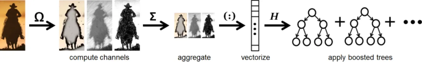
Fig. 8. Overview of the ACF detector. Given an input imageI, we compute several channelsC= Ω(I), sum every block of pixels inC, and smooth the resulting lower resolution channels. Features are single pixel lookups in the aggregated channels. Boosting is used to learn decision trees over these features (pixels) to distinguish object from background. With the appropriate choice of channels and careful attention to design, ACF achieves state-of-the-art performance in pedestrian detection.

Alternate schemes, such as interpolating between two nearby scaless0_{for each intermediate scalesor} evaluat-ingΩmore densely, could result in even higher pyramid accuracy (at increased cost). However, the proposed approach proves sufficient for object detection (see §6). 5.3 Complexity Analysis

The computational savings of computing approximate feature pyramids is significant. Assume the cost of com-puting Ω is linear in the number of pixels in an n×n image (as is often the case). The cost of constructing a feature pyramid with mscales per octave is:

∞ X k=0 n22−2k/m=n2 ∞ X k=0 (4−1/m)k= n 2 1−4−1/m ≈ mn2 ln 4 (8)

The second equality follows from the formula for a sum of a geometric series; the last approximation is valid for large m (and follows from l’H ˆopital’s rule). In the proposed approach we compute Ω once per octave (m = 1). The total cost is 4

3n

2_{, which is only 33% more} than the cost of computing single scale features. Typical detectors are evaluated on8to12scales per octave [31], thus according to (8) we achieve an order of magnitude savings over computingΩdensely (and intermediateCs are computed efficiently through resampling afterward).

6

A

PPLICATIONS TO

O

BJECT

D

ETECTION We demonstrate the effectiveness of fast feature pyra-mids in the context of object detection with three dis-tinct detection frameworks. First, in §6.1 we show the efficacy of our approach with a simple yet state-of-the-art pedestrian detector we introduce in this work called Aggregated Channel Features(ACF). In§6.2we describe an alternate approach for exploiting approximate multiscale features using integral images computed over the same channels (Integral Channel Features or ICF), much as in our previous work [29], [39]. Finally, in§6.3we approxi-mate HOG feature pyramids for use withDeformable Part Models (DPM) [35].

6.1 Aggregated Channel Features (ACF)

The ACF detection framework is conceptually straight-forward (Figure8). Given an input imageI, we compute several channelsC= Ω(I), sum every block of pixels in C, and smooth the resulting lower resolution channels.

Features are single pixel lookups in the aggregated chan-nels. Boosting is used to train and combine decision trees over these features (pixels) to distinguish object from background and a multiscale sliding-window approach is employed. With the appropriate choice of channels and careful attention to design, ACF achieves state-of-the-art performance in pedestrian detection.

Channels: ACF uses the same channels as [39]: nor-malized gradient magnitude, histogram of oriented gra-dients (6 channels), and LUV color channels. Prior to computing the 10 channels, I is smoothed with a [1 2 1]/4 filter. The channels are divided into 4 × 4

blocks and pixels in each block are summed. Finally the channels are smoothed, again with a [1 2 1]/4 filter. For

640×480 images, computing the channels runs at over 100 fpson a modern PC. The code is optimized but runs on a single CPU; further gains could be obtained using multiple cores or a GPU as in [30].

Pyramid: Computation of feature pyramids at octave-spaced scale intervals runs at ∼_{75 fps on} 640 ×480

images. Meanwhile, computing exact feature pyramids with eight scales per octave slows to∼_{15 fps, precluding} real-time detection. In contrast, our fast pyramid con-struction (see§5) with 7 of 8 scales per octave approxi-mated runs at nearly50 fps.

Detector: For pedestrian detection, AdaBoost [69] is used to train and combine 2048 depth-two trees over the

128·64·10/16 = 5120candidate features (channel pixel lookups) in each128×64window. Training with multiple rounds of bootstrapping takes ∼_{10 minutes (a parallel} implementation reduces this to∼_{3 minutes). The detector} has a step size of 4 pixels and 8 scales per octave. For 640 ×480 images, the complete system, including fast pyramid construction and sliding-window detection, runs at over 30 fps allowing for real-time uses (with exact feature pyramids the detector slows to 12 fps).

Code: Code for the ACF framework is available on-line4. For more details on the channels and detector used in ACF, including exact parameter settings and training framework, we refer users to the source code.

Accuracy: We report accuracy of ACF with exact and fast feature pyramids in Table1. Following the method-ology of [31], we summarize performance using the log-average miss rate (MR) between10−2 and100_false pos-itives per image. Results are reported on four pedestrian datasets: INRIA [21], Caltech [31], TUD-Brussels [36] and

INRIA [21] Caltech [31] TUD [36] ETH [37] MEAN Shapelet [70] 82 91 95 91 90 VJ [27] 72 95 95 90 88 PoseInv [71] 80 86 88 92 87 HikSvm [72] 43 73 83 72 68 HOG [21] 46 68 78 64 64 HogLbp [73] 39 68 82 55 61 MF [74] 36 68 73 60 59 PLS [75] 40 62 71 55 57 MF+CSS [76] 25 61 60 61 52 MF+Motion [76] – 51 55 60 – LatSvmV2 [35] 20 63 70 51 51 FPDW [39] 21 57 63 60 50 ChnFtrs [29] 22 56 60 57 49 Crosstalk [40] 19 54 58 52 46 VeryFast [30] 16 – – 55 – MultiResC [77] – 48 – – – ICF-Exact§6.2 18 48 53 50 42 ICF§6.2 19 51 55 56 45 ACF-Exact§6.1 17 43 50 50 40 ACF§6.1 17 45 52 51 41 TABLE 1

MRs of leading approaches for pedestrian detection on four datasets. For ICF and ACF exact and approximate detection results are shown with only small differences between them. For the latest pedestrian detection results please see [32].

ETH [37]. MRs for 16 competing methods are shown. ACF outperforms competing approaches on nearly all datasets. When averaged over the four datasets, the MR of ACF is 40% with exact feature pyramids and 41% with fast feature pyramids, a negligible difference, demonstrating the effectiveness of our approach.

Speed: MR versus speed for numerous detectors is shown in Figure 10. ACF with fast feature pyramids runs at ∼_{32 fps. The only two faster approaches are} Crosstalk cascades [40] and the VeryFast detector from Benenson et al. [30]. Their additional speedups are based on improved cascade strategies and combining multi-resolution models with a GPU implementation, respec-tively, and are orthogonal to the gains achieved by using approximate multiscale features. Indeed, all the detectors that run at 5 fps and higher exploit the power law governing feature scaling.

Pyramid parameters: Detection performance on IN-RIA [21] with fast feature pyramids under varying set-tings is shown in Figure11. The key result is given in Fig-ure 11(a): when approximating 7 of 8 scales per octave, the MR for ACF is .169 which is virtually identical to the MR of.166obtained using the exact feature pyramid. Even approximating 15 of every 16 scales increases MR only somewhat. Constructing the channels without cor-recting for power law scaling, or using an incorrect value of λ, results in markedly decreased performance, see Figure11(b). Finally, we observe that at least 8 scales per octave must be used for good performance (Figure11(c)), making the proposed scheme crucial for achieving detec-tion results that are both fast and accurate.

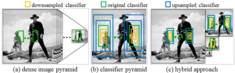
Fig. 9. (a) A standard pipeline for performing multiscale de-tection is to create a densely sampled feature pyramid.(b)Viola and Jones [27] used simple shift and scale invariant features, al-lowing a detector to be placed at any location and scale without relying on a feature pyramid.(c)ICF can use a hybrid approach of constructing an octave-spaced feature pyramid followed by approximating detector responses within half an octave of each pyramid level.

6.2 Integral Channel Features (ICF)

Integral Channel Features (ICF) [29] are a precursor to the ACF framework described in§6.1. Both ACF and ICF use the same channel features and boosted classifiers; the key difference between the two frameworks is that ACF uses pixel lookups in aggregated channels as features while ICF uses sums over rectangular channel regions (computed efficiently with integral images).

Accuracy of ICF with exact and fast feature pyramids is shown in Table1. ICF achieves state-of-the-art results: inferior to ACF but otherwise outperforming most com-peting approaches. The MR of ICF averaged over the four datasets is 42% with exact feature pyramids and 45% with fast feature pyramids. The gap of 3% is larger than the 1% gap for ACF but still small. With fast feature pyramids ICF runs at ∼_{16 fps, see Figure 10. ICF is} slower than ACF due to construction of integral images and more expensive features (rectangular sums com-puted via integral images versus single pixel lookups). For more details on ICF, see [29], [39]. The variant tested here uses identical channels to ACF.

Detection performance with fast feature pyramids un-der varying settings is shown in Figure 12. The plots mirror the results shown in Figure 11for ACF. The key result is given in Figure12(a): when approximating 7 of 8 scales per octave, the MR for ICF is 2% worse than the MR obtained with exact feature pyramids.

The ICF framework allows for an alternate application of the power law governing feature scaling: instead of rescaling channels as discussed in §5, one can instead rescale the detector. Using the notation from §4, rectan-gular channel sums (features used in ICF) can be written as AfΩ(I), where A denotes rectangle area. As such, Eqn. (4) can be applied to approximate features at nearby scales and given integral channel images computed at one scale, detector responses can be approximated at nearby scales. This operation can be implemented by rescaling the detector itself, see [39]. As the approxima-tion degrades with increasing scale offsets, a hybrid ap-proach is to construct an octave-spaced feature pyramid followed by approximating detector responses at nearby scales, see Figure9. This approach was extended in [30].

1/64 1/32 1/16 1/8 1/4 1/2 1 2 4 8 16 32 64 .15 .20 .30 .40 .50 .64 .80 A B C D E F GH I J K L M N O P Q

frames per second

log−average miss rate

A Pls B MultiFtr+CSS C Shapelet D HogLbp E MultiFtr F FtrMine G HikSvm H HOG I LatSvm−V1 J PoseInv K [20.0%/0.6fps] LatSvm−V2 L [22.0%/1.2fps] ChnFtrs M [21.0%/6.5fps] FPDW N [19.7%/16.4fps] ICF O [17.0%/31.9fps] ACF P [20.1%/45.4fps] Crosstalk Q [16.0%/50.0fps] VeryFast

Fig. 10. Log-average miss rate (MR) on the INRIA pedestrian dataset [21] versus frame rate on640×480images for multiple detectors. Method runtimes were obtained from [31], see also [31] for citations for detectors A-L. Numbers in brackets indicate MR/fps for select approaches, sorted by speed. All detectors that run at 5 fps and higher are based on our fast feature pyramids; these methods are also the most accurate.They include: (M) FPDW [39] which is our original implementation of ICF, (N) ICF [§6.2], (O) ACF [§6.1], (P) crosstalk cascades [40], and (Q) the VeryFast detector from Benenson et al. [30]. Both (P) and (Q) use the power law governing feature scaling described in this work; the additional speedups in (P) and (Q) are based on improved cascade strategies, multi-resolution models and a GPU implementation, and are orthogonal to the gains achieved by using approximate multiscale features.

(a) fraction approximated scales (b)λfor normalized gradient channels (c) scales per octave

Fig. 11. Effect of parameter setting of fast feature pyramids on theACFdetector [§6.1]. We report log-average miss rate (MR) averaged over 25 trials on the INRIA pedestrian dataset [21]. Orange diamonds denote default parameter settings: 7/8 scales approximated per octave,λ≈.17for the normalized gradient channels, and 8 scales per octave in the pyramid. (a) The MR stays relatively constant as the fraction of approximated scales increases up to 7/8 demonstrating the efficacy of the proposed approach.(b)Sub-optimal values ofλwhen approximating the normalized gradient channels cause a marked decrease in performance.(c)At least 8 scales per octave are necessary for good performance, making the proposed scheme crucial for achieving detection results that are both fast and accurate.

(a) fraction approximated scales (b)λfor normalized gradient channels (c) scales per octave

Fig. 12. Effect of parameter setting of fast feature pyramids on theICFdetector [§6.2]. The plots mirror the results shown in Figure11for the ACF detector, although overall performance for ICF is slightly lower.(a)When approximating 7 of every 8 scales in the pyramid, the MR for ICF is.195which is only slightly worse than the MR of.176obtained using exact feature pyramids.(b)Computing approximate channels with an incorrect value ofλresults in decreased performance (although using a slightly largerλthan predicted appears to improve results marginally).(c)Similarly to the ACF framework, at least 8 scales per octave are necessary to achieve good results.

plane bike bird boat bottle bus car cat chair cow DPM 26.3 59.4 2.3 10.2 21.2 46.2 52.2 7.9 15.9 17.4 ∼_{DPM 24.1 54.7 1.6 9.8 20.0 42.1 50.1 8.0 13.8 16.7} table dog horse moto person plant sheep sofa train tv DPM 10.9 2.9 53.4 37.6 38.2 4.9 16.6 29.7 38.2 40.8 ∼_{DPM 8.9 2.5 49.4 38.3 36.0 4.2 14.9 24.4 35.8 35.0}

TABLE 2

Average precision scores for deformable part models with exact (DPM) and approximate (∼DPM) feature pyramids on PASCAL.

6.3 Deformable Part Models (DPM)

Deformable Part Models (DPM) from Felzenszwalb et al. [35] are an elegant approach for general object detection that have consistently achieved top results on the PAS-CAL VOC challenge [38]. DPMs use a variant of HOG features [21] as their image representation, followed by classification with linear SVMs. An object model is composed of multiple parts, a root model, and optionally multiple mixture components. For details see [35].

Recent approaches for increasing the speed of DPMs include work by Felzenszwalb et al. [44] and Pedersoli et al. [45] on cascaded and coarse-to-fine deformable part models, respectively. Our work is complementary as we focus on improving the speed of pyramid construction. The current bottleneck of DPMs is in the classification stage, therefore pyramid construction accounts for only a fraction of total runtime. However, if fast feature pyra-mids are coupled with optimized classification schemes [44], [45], DPMs have the potential to have more com-petitive runtimes. We focus on demonstrating DPMs can achieve good accuracy with fast feature pyramids and leave the coupling of fast feature pyramids and optimized classification schemes to practitioners.

DPM code is available online [35]. We tested pre-trained DPM models on the 20 PASCAL 2007 categories using exact HOG pyramids and HOG pyramids with 9 of 10 scales per octave approximated using our proposed approach. Average precision (AP) scores for the two approaches, denoted DPM and ∼_{DPM, respectively, are} shown in Table2. The mean AP across the 20 categories is 26.6% for DPMs and 24.5% for ∼_{DPMs. Using fast} HOG feature pyramids only decreased mean AP 2%, demonstrating the validity of the proposed approach.

7

C

ONCLUSION

Improvements in the performance of visual recognition systems in the past decade have in part come from the realization that finely sampled pyramids of image features provide a good front-end for image analysis. It is widely believed that the price to be paid for improved performance is sharply increased computational costs. We have shown that this is not necessarily so. Finely sampled pyramids may be obtained inexpensively by extrapolation from coarsely sampled ones. This insight decreases computational costs substantially.

Our insight ultimately relies on the fractal structure of much of the visual world. By investigating the statistics of natural images we have demonstrated that the be-havior of image features can be predicted reliably across scales. Our calculations and experiments show that this makes it possible to estimate features at a given scale inexpensively by extrapolating computations carried out at a coarsely sampled set of scales. While our results do not hold under all circumstances, for instance, on images of textures or white noise, they do hold for images typically encountered in the natural world.

In order to validate our findings we studied the per-formance of three end-to-end object detection systems. We found that detection rates are relatively unaffected while computational costs decrease considerably. This has led to the first detectors that operate at frame rate while using rich feature representations.

Our results are not restricted to object detection nor to visual recognition. The foundations we have devel-oped should readily apply to other computer vision tasks where a fine-grained scale sampling of features is necessary as the image processing front end.

A

CKNOWLEDGMENTS

We would like to thank Peter Welinder and Rodrigo Be-nenson for helpful comments and suggestions. P. Doll´ar, R. Appel, and P. Perona were supported by MURI-ONR N00014-10-1-0933 and ARO/JPL-NASA Stennis NAS7.03001. R. Appel was also supported by NSERC 420456-2012 and The Moore Foundation. S. Belongie was supported by NSF CAREER Grant 0448615, MURI-ONR N00014-08-1-0638 and a Google Research Award.

R

EFERENCES

[1] D. Hubel and T. Wiesel, “Receptive fields and functional archi-tecture of monkey striate cortex,”Journal of Physiology, 1968. [2] C. Malsburg, “Self-organization of orientation sensitive cells in

the striate cortex,”Biological Cybernetics, vol. 14, no. 2, 1973. [3] L. Maffei and A. Fiorentini, “The visual cortex as a spatial

frequency analyser,”Vision Research, vol. 13, no. 7, 1973. [4] P. Burt and E. Adelson, “The laplacian pyramid as a compact

image code,”IEEE Transactions on Communications, 1983. [5] J. Daugman, “Uncertainty relation for resolution in space, spatial

frequency, and orientation optimized by two-dimensional visual cortical filters,”Journal of the Optical Society of America A, 1985. [6] J. Koenderink and A. Van Doorn, “Representation of local

geome-try in the visual system,”Biological cybernetics, vol. 55, no. 6, 1987. [7] D. J. Field, “Relations between the statistics of natural images and the response properties of cortical cells,”Journal of the Optical Society of America A, vol. 4, pp. 2379–2394, 1987.

[8] S. Mallat, “A theory for multiresolution signal decomposition: the wavelet representation,”PAMI, vol. 11, no. 7, 1989.

[9] P. Vaidyanathan, “Multirate digital filters, filter banks, polyphase networks, and applications: A tutorial,” Proceedings of the IEEE, vol. 78, no. 1, 1990.

[10] M. Vetterli, “A theory of multirate filter banks,”IEEE Conference on Acoustics, Speech and Signal Processing, vol. 35, no. 3, 1987. [11] E. Simoncelli and E. Adelson, “Noise removal via bayesian

wavelet coring,” inICIP, vol. 1, 1996.

[12] W. T. Freeman and E. H. Adelson, “The design and use of steerable filters,”PAMI, vol. 13, pp. 891–906, 1991.

[13] J. Malik and P. Perona, “Preattentive texture discrimination with early vision mechanisms,”Journal of the Optical Society of America A, vol. 7, pp. 923–932, May 1990.

[14] D. Jones and J. Malik, “Computational framework for determin-ing stereo correspondence from a set of linear spatial filters,” Image and Vision Computing, vol. 10, no. 10, pp. 699–708, 1992. [15] E. Adelson and J. Bergen, “Spatiotemporal energy models for the

perception of motion,”Journal of the Optical Society of America A, vol. 2, no. 2, pp. 284–299, 1985.

[16] Y. Weiss and E. Adelson, “A unified mixture framework for mo-tion segmentamo-tion: Incorporating spatial coherence and estimating the number of models,” inCVPR, 1996.

[17] L. Itti, C. Koch, and E. Niebur, “A model of saliency-based visual attention for rapid scene analysis,”PAMI, vol. 20, no. 11, 1998. [18] P. Perona and J. Malik, “Detecting and localizing edges composed

of steps, peaks and roofs,” inICCV, 1990.

[19] M. Lades, J. Vorbruggen, J. Buhmann, J. Lange, C. von der Malsburg, R. Wurtz, and W. Konen, “Distortion invariant object recognition in the dynamic link architecture,”IEEE Transactions on Computers, vol. 42, no. 3, pp. 300–311, 1993.

[20] D. G. Lowe, “Object recognition from local scale-invariant fea-tures,” inICCV, 1999.

[21] N. Dalal and B. Triggs, “Histograms of oriented gradients for human detection,” inCVPR, 2005.

[22] R. De Valois, D. Albrecht, and L. Thorell, “Spatial frequency selectivity of cells in macaque visual cortex,” Vision Research, vol. 22, no. 5, pp. 545–559, 1982.

[23] Y. LeCun, P. Haffner, L. Bottou, and Y. Bengio, “Gradient-based learning applied to document recognition,” inProc. of IEEE, 1998. [24] M. Riesenhuber and T. Poggio, “Hierarchical models of object

recognition in cortex,”Nature Neuroscience, vol. 2, 1999.

[25] D. G. Lowe, “Distinctive image features from scale-invariant keypoints,”IJCV, vol. 60, no. 2, pp. 91–110, 2004.

[26] A. Krizhevsky, I. Sutskever, and G. Hinton, “Imagenet classifica-tion with deep convoluclassifica-tional neural networks,” inNIPS, 2012. [27] P. Viola and M. Jones, “Rapid object detection using a boosted

cascade of simple features,” inCVPR, 2001.

[28] P. Viola, M. Jones, and D. Snow, “Detecting pedestrians using patterns of motion and appearance,”IJCV, vol. 63(2), 2005. [29] P. Doll´ar, Z. Tu, P. Perona, and S. Belongie, “Integral channel

features,” inBMVC, 2009.

[30] R. Benenson, M. Mathias, R. Timofte, and L. Van Gool, “Pedestrian detection at 100 frames per second,” inCVPR, 2012.

[31] P. Doll´ar, C. Wojek, B. Schiele, and P. Perona, “Pedestrian detec-tion: An evaluation of the state of the art,”PAMI, vol. 99, 2011. [32] www.vision.caltech.edu/Image Datasets/CaltechPedestrians/. [33] D. L. Ruderman and W. Bialek, “Statistics of natural images:

Scaling in the woods,”Physical Review Letters, vol. 73, no. 6, pp. 814–817, Aug 1994.

[34] E. Switkes, M. Mayer, and J. Sloan, “Spatial frequency analysis of the visual environment: anisotropy and the carpentered environ-ment hypothesis,”Vision Research, vol. 18, no. 10, 1978.

[35] P. Felzenszwalb, R. Girshick, D. McAllester, and D. Ramanan, “Object detection with discriminatively trained part based mod-els,”PAMI, vol. 32, no. 9, pp. 1627–1645, 2010.

[36] C. Wojek, S. Walk, and B. Schiele, “Multi-cue onboard pedestrian detection,” inCVPR, 2009.

[37] A. Ess, B. Leibe, and L. Van Gool, “Depth and appearance for mobile scene analysis,” inICCV, 2007.

[38] M. Everingham, L. Van Gool, C. K. I. Williams, J. Winn, and A. Zis-serman, “The PASCAL visual object classes (VOC) challenge,” IJCV, vol. 88, no. 2, pp. 303–338, Jun. 2010.

[39] P. Doll´ar, S. Belongie, and P. Perona, “The fastest pedestrian detector in the west,” inBMVC, 2010.

[40] P. Doll´ar, R. Appel, and W. Kienzle, “Crosstalk cascades for frame-rate pedestrian detection,” inECCV, 2012.

[41] T. Lindeberg, “Scale-space for discrete signals,” PAMI, vol. 12, no. 3, pp. 234–254, 1990.

[42] J. L. Crowley, O. Riff, and J. H. Piater, “Fast computation of characteristic scale using a half-octave pyramid,” inInternational Conference on Scale-Space Theories in Computer Vision, 2002. [43] R. S. Eaton, M. R. Stevens, J. C. McBride, G. T. Foil, and M. S.

Snorrason, “A systems view of scale space,” inICVS, 2006. [44] P. Felzenszwalb, R. Girshick, and D. McAllester, “Cascade object

detection with deformable part models,” inCVPR, 2010. [45] M. Pedersoli, A. Vedaldi, and J. Gonzalez, “A coarse-to-fine

approach for fast deformable object detection,” inCVPR, 2011. [46] C. H. Lampert, M. B. Blaschko, and T. Hofmann, “Efficient

subwindow search: A branch and bound framework for object localization,”PAMI, vol. 31, pp. 2129–2142, Dec 2009.

[47] L. Bourdev and J. Brandt, “Robust object detection via soft cascade,” inCVPR, 2005.

[48] C. Zhang and P. Viola, “Multiple-instance pruning for learning efficient cascade detectors,” inNIPS, 2007.

[49] J. ˇSochman and J. Matas, “Waldboost - learning for time con-strained sequential detection,” inCVPR, 2005.

[50] H. Masnadi-Shirazi and N. Vasconcelos, “High detection-rate cascades for real-time object detection,” inICCV, 2007.

[51] F. Fleuret and D. Geman, “Coarse-to-fine face detection,”IJCV, vol. 41, no. 1-2, pp. 85–107, 2001.

[52] P. Felzenszwalb and D. Huttenlocher, “Efficient matching of pic-torial structures,” inCVPR, 2000.

[53] C. Papageorgiou and T. Poggio, “A trainable system for object detection,”IJCV, vol. 38, no. 1, pp. 15–33, 2000.

[54] M. Weber, M. Welling, and P. Perona, “Unsupervised learning of models for recognition,” inECCV, 2000.

[55] S. Agarwal and D. Roth, “Learning a sparse representation for object detection,” inECCV, 2002.

[56] R. Fergus, P. Perona, and A. Zisserman, “Object class recognition by unsupervised scale-invariant learning,” inCVPR, 2003. [57] B. Leibe, A. Leonardis, and B. Schiele, “Robust object detection

with interleaved categorization and segmentation,”IJCV, vol. 77, no. 1-3, pp. 259–289, May 2008.

[58] C. Gu, J. J. Lim, P. Arbel´aez, and J. Malik, “Recognition using regions,” inCVPR, 2009.

[59] B. Alexe, T. Deselaers, and V. Ferrari, “What is an object?” in CVPR, 2010.

[60] C. Wojek, G. Dork ´o, A. Schulz, and B. Schiele, “Sliding-windows for rapid object class localization: A parallel technique,” in DAGM, 2008.

[61] L. Zhang and R. Nevatia, “Efficient scan-window based object detection using gpgpu,” in Visual Computer Vision on GPU’s (CVGPU), 2008.

[62] B. Bilgic, “Fast human detection with cascaded ensembles,” Mas-ter’s thesis, MIT, February 2010.

[63] Q. Zhu, S. Avidan, M. Yeh, and K. Cheng, “Fast human detection using a cascade of histograms of oriented gradients,” in CVPR, 2006.

[64] F. M. Porikli, “Integral histogram: A fast way to extract histograms in cartesian spaces,” inCVPR, 2005.

[65] A. Ess, B. Leibe, K. Schindler, and L. Van Gool, “Robust multi-person tracking from a mobile platform,”PAMI, vol. 31, pp. 1831– 1846, 2009.

[66] M. Bajracharya, B. Moghaddam, A. Howard, S. Brennan, and L. H. Matthies, “A fast stereo-based system for detecting and tracking pedestrians from a moving vehicle,”The International Journal of Robotics Research, vol. 28, 2009.

[67] D. L. Ruderman, “The statistics of natural images,” Network: Computation in Neural Systems, vol. 5, no. 4, pp. 517–548, 1994. [68] S. G. Ghurye, “A characterization of the exponential function,”

The American Mathematical Monthly, vol. 64, no. 4, 1957.

[69] J. Friedman, T. Hastie, and R. Tibshirani, “Additive logistic re-gression: a statistical view of boosting,” The Annals of Statistics, vol. 38, no. 2, pp. 337–374, 2000.

[70] P. Sabzmeydani and G. Mori, “Detecting pedestrians by learning shapelet features,” inCVPR, 2007.

[71] Z. Lin and L. S. Davis, “A pose-invariant descriptor for human detection and segmentation,” inECCV, 2008.

[72] S. Maji, A. Berg, and J. Malik, “Classification using intersection kernel SVMs is efficient,” inCVPR, 2008.

[73] X. Wang, T. X. Han, and S. Yan, “An hog-lbp human detector with partial occlusion handling,” inICCV, 2009.

[74] C. Wojek and B. Schiele, “A performance evaluation of single and multi-feature people detection,” inDAGM, 2008.

[75] W. Schwartz, A. Kembhavi, D. Harwood, and L. Davis, “Human detection using partial least squares analysis,” inICCV, 2009. [76] S. Walk, N. Majer, K. Schindler, and B. Schiele, “New features and

insights for pedestrian detection,” inCVPR, 2010.

[77] D. Park, D. Ramanan, and C. Fowlkes, “Multiresolution models for object detection,” inECCV, 2010.

Piotr Doll ´ar received his masters degree in computer science from Harvard University in 2002 and his PhD from the University of Califor-nia, San Diego in 2007. He joined the Compu-tational Vision lab at Caltech as a postdoctoral fellow in 2007. Upon being promoted to senior postdoctoral fellow he realized it time to move on, and in 2011, he joined the Interactive Visual Media Group at Microsoft Research, Redmond, where he currently resides. He has worked on object detection, pose estimation, boundary learning and behavior recognition. His general interests lie in machine learning and pattern recognition and their application to computer vision.

Ron Appelis completing his PhD in the Compu-tational Vision lab at Caltech, where he currently holds an NSERC graduate award. He received his bachelors and masters degrees in 2006 and 2008 in electrical and computer engineering from the University of Toronto, and co-founded ViewGenie inc., a company specializing in intelli-gent image processing and search. His research interests include machine learning, visual object detection, and algorithmic optimization.

Serge Belongie received a BS (with honor) in EE from Caltech in 1995 and a PhD in EECS from Berkeley in 2000. While at Berkeley, his research was supported by an NSF Gradu-ate Research Fellowship. From 2001-2013 he was a professor in the Department of Com-puter Science and Engineering at UCSD. He is currently a professor at Cornell NYC Tech and the Cornell Computer Science Department. His research interests include Computer Vision, Machine Learning, Crowdsourcing and Human-in-the-Loop Computing. He is also a co-founder of several companies including Digital Persona, Anchovi Labs (acquired by Dropbox) and Orpix. He is a recipient of the NSF CAREER Award, the Alfred P. Sloan Research Fellowship and the MIT Technology Review “Innovators Under 35” Award.

Pietro Peronagraduated in Electrical Engineer-ing from the Universit `a di Padova in 1985 and received a PhD in Electrical Engineering and Computer Science from the University of Cali-fornia at Berkeley in 1990. After a postdoctoral fellowship at MIT in 1990-91 he joined the faculty of Caltech in 1991, where he is now an Allen E. Puckett Professor of Electrical Engineering and Computation and Neural Systems. His current interests are visual recognition, modeling vision in biological systems, modeling and measur-ing behavior, and Visipedia. He has worked on anisotropic diffusion, multiresolution-multi-orientation filtering, human texture perception and segmentation, dynamic vision, grouping, analysis of human motion, recognition of object categories, and modeling visual search.