Deep Learning For Multimedia
Processing
-Predicting Media Interestingness
Degree’s Thesis
Cience and Technologies of Telecommunications Engineering
Author: Lluc Cardoner Campi
Advisors: Xavier Gir´o-i-Nieto, Maia Zaharieva
Universitat Polit`ecnica de Catalunya (UPC) 2016 - 2017
Abstract
This thesis explores the application of a deep learning approach for the prediction of media interestingness. Two different models are investigated, one for the prediction of image and one for the prediction of video interestingness.
For the prediction of image interestingness, the ResNet50 network is fine-tuned to obtain best results. First, some layers are added. Next, the model is trained and fine-tuned using data augmentation, dropout, class weights, and changing other hyper parameters.
For the prediction of video interestingness, first, features are extracted with a 3D convolutional network. Next a LSTM network is trained and fine-tuned with the features.
The final result is a binary label for each image/video: 1 for interesting, 0 for not interesting. Additionally, a confidence value is provided for each prediction. Finally, the Mean Average Precision (MAP) is employed as evaluation metric to estimate the quality of the final results.
Resum
Aquesta t`esi explora un enfocament ambdeep learning aplicat a la predicci´o del nivell d’inter`es d’imatges i v´ıdeos. S’investiguen dos models, un per a predir el nivell d’inter`es d’imatges i un altre per a v´ıdeos.
Per a la predicci´o del nivell d’inter`es d’imatges, s’adapta la xarxa ResNet50 amb la finalitat d’obtenir els millors resultats. En primer lloc, s’afegeixen capes. A continuaci´o, s’entrena i s’adapta el model utilitzant augmentaci´o de les dades,dropout, ponderaci´o de classes i canviant hiperpar`ametres.
Per a la predicci´o del nivell d´ınter`es de v´ıdeos, en primer lloc, s’extreuen caracter´ıstiques dels v´ıdeos amb una xarxa convolucional 3D. A continuaci´o, s’entrena i s’adapta una xarxa LSTM amb aquestes caracter´ıstiques.
El resultat final ´es una classificaci´o bin`aria de cada imatge/v´ıdeo: 1 per a ”interessant”, 0 per a ”no interessant”. A m´es a m´es, s’aporta un nivell de confian¸ca a cada predicci´o. Finalment, el promig de la precisi´o mitja (MAP) s’utilitza com a m`etrica d’evaluaci´o per a estimar la qualitat dels resultats finals.
Resumen
Esta tesis explora un enfoque condeep learning aplicado a la predicci´on del nivel de inter´es de im´agenes y videos. Se investigan dos modelos, uno para predecir el nivel de inter´es de imagenes y otro para v´ıdeos.
Para la predicci´on del nivel de inter´es de im´agenes, se adapta la red ResNet50 con el fin de obtener los mejores resultados. En primer lugar, se a˜naden capas. A continuaci´on, se entrena y se adapta el modelo utilizando aumento de datos, dropout, ponderaci´on de classes y cambiando otros hiperpar´ametros.
Para la predicci´on del nivel de inter´es de v´ıdeos, en primer lugar, se extraen caracter´ısticas de los v´ıdeos con una red convolucional 3D. A continuaci´on se entrena y se adapta una red LSTM con estas caracter´ısticas.
El resultado final es una classificaci´on binaria para cada imagen/v´ıdeo: 1 para ”interesante”, 0 para ”no interesante”. Adem´as, se aporta un nivel de confianza en cada predicci´on. Finalmente, el promedio de la precisi´on media (MAP) se usa como m´etrica de evaluaci´on para estimar la calidad de los resultados finales.
Acknowledgements
I want to thank my advisors, Xavier and Maia, for the continuous help and support through all the project process. Thanks for guiding me and assisting me in the difficult moments.
I would also like to thanks Alverto Montes for his help and knowledge in video processing and making his code available.
Also I appreciate my friends for supporting me.
Revision history and approval record
Revision Date Purpose
0 5/06/2017 Document creation 1 30/6/2017 Document revision
DOCUMENT DISTRIBUTION LIST
Name e-mail
Lluc Cardoner Campi [email protected] Xavier Gir´o i Nieto [email protected]
Maia Zaharieva [email protected]
Written by: Reviewed and approved by:
Date 5/6/2017 Date 30/6/2017
Name Lluc Cardoner Name Xavier Gir´o
Contents
1 Introduction 10
1.1 Statement of purpose . . . 10
1.2 Requirements and specifications . . . 10
1.3 Methods and procedures . . . 11
1.4 Work Plan . . . 12
1.4.1 Work Packages . . . 12
1.4.2 Gantt Diagram . . . 13
1.5 Incidents and Modification . . . 14
2 State of the art 15 2.1 Media interestingness . . . 15
2.2 Previous year’s task . . . 15
2.2.1 Features . . . 16 2.2.2 Models . . . 16 3 Methodology 18 3.1 Dataset . . . 18 3.1.1 Precomputed features . . . 18 3.1.2 Data . . . 19 3.1.3 Ground truth . . . 19
3.2 Predicting Image Interestingness . . . 21
3.2.1 Fine-tuning ResNet50 . . . 21
3.2.1.1 Adding layers . . . 21
3.2.1.2 Data augmentation . . . 22
3.2.1.3 Dropout . . . 23
3.2.1.5 Train last layers ResNet50 . . . 25
3.2.1.6 Classifier with SVM . . . 25
3.3 Predicting Video Interestingness . . . 25
3.3.1 Extract features: C3D . . . 26
3.3.2 Fine-tuning LSTM network . . . 28
4 Results 30 4.1 Evaluation metric . . . 30
4.2 Baseline . . . 30
4.3 Image interestingness results . . . 30
4.4 Video interestingness results . . . 32
5 Budget 35
6 Conclusions 36
List of Figures
1.1 Gantt Diagram of the Degree Thesis . . . 13
3.1 Example of interesting images (top row) and not interesting images (bottom row) with their [classification, interestingness value, and ranking] within its video respectively. . . 20
3.2 Ground truth labels of the segments of one video. Note that all the frames of one segment have the same label and the segments have different lengths. . . 20
3.3 Architecture of the network after adding layers. . . 22
3.4 Architecture of the network after adding dropout. . . 23
3.5 Number of samples of training set with label 0 for not interesting and 1 for
interesting . . . 24 3.6 Preprocessing of the video segments for feature extraction with the C3D. . . 26
3.7 Architecture of the pipeline for predicting video interestingness. . . 28
4.1 Training labels (red) and predictions (green) of the feature vector labels for one video. x axes - feature vectors, y axes - interestingness value . . . 32
List of Tables
3.1 Structure of 2016 and 2017 dataset . . . 19
4.1 Baseline and top results of 2016 for predicting image and video interestingness . 30 4.2 Best MAP results of fine-tuning the ResNet50 with 0.5 threshold . . . 31
4.3 Best MAP results of fine-tuning the ResNet50 with dynamic threshold . . . 31
4.4 MAP results using a SVM classifier . . . 32
4.5 Result for predicting video interestingness with the LSTM network . . . 34
Chapter 1
Introduction
1.1
Statement of purpose
The ability of multimedia data to attract and keep people’s interest for long periods of time is gaining more and more importance in the field of multimedia. Still, no common definition for interestingness exists in the research community. Related works exploring interestingness are also related to aesthetics, popularity, and memorability. They all have in common the analyzis of a subjective aspect of media.
This project is motivated by the MediaEval Predicting Media Interestingness task1. MediaEval is a benchmarking initiative which facilitates the comparability of approaches solving real-world multimedia tasks. The Predicting Media Interestingness Task was proposed for the first time last year (2016). This year’s edition is a follow-up which builds incrementally upon the previous experience.
The purpose of this work is to predict interestingness of images and videos. This task is driven by the requirements of a Video on Demand (VOD) web site. The more interesting the frames or the video sequences are, which are shown to the user, the more likely he/she will watch the corresponding movie. The aim of the project is to provide a system that classifies an image or a video sequence in interesting or non-interesting along with a confidence value. In order to solve this task, state-of-the-art deep learning techniques are explored to achieve best results. In particular, the main contributions of this project are:
• Training and fine-tunning of the ResNet50 network for predicting image interestingness.
• Training and fine-tunning of a LSTM network for predicting video interestingness.
This project has been developed at the TU Wien during the Spring semester of 2017.
1.2
Requirements and specifications
This project has been developed to actively participate in the MediaEval Predicting Media Interestingness task 2017. The official task requirements for the project are:
• The task is a binary classification task: interesting or not interesting.
• A confidence value is required for each prediction.
• The official evaluation metric is the Mean Average Precision: MAP (See section 4.1).
1
The only additional requirement for the project is that a end-to-end deep learning architecture has to be used. This specification does not come from Mediaeval, instead it was agreed with the advisors. No other specifications were defined. The project has been developed entirely in Python due to the use of the Keras framework2. Keras is a high-level neural networks API written in Python and capable of running on the top of either TensorFlow3 or Theano4. For this project TensorFlow has been used since some of the models used are available on it.
In addition to the software, a GPU was required due to the high demanding computational power needed to train a neural network. A local computer fromTU Wienwith a GPU was used.
1.3
Methods and procedures
Different deep learning models have been explored for predicting image and video interesting-ness. The baselines for the image and video tasks are explained in Section 4.2.
The model used for predicting image interestingness is the ResNet50 network. This network was fine-tunned to obtain the best results with the given data. This solution first removed the class classification layer from ResNet50 and, next, added one fully-connected layer with 2 neurons with softmax activation to obtain the probabilities for each class. The two classes are:
1 for interesting and 0 for non-interesting. In following, several experiments were performed in order to fine-tune the network.
The different experiments considered the following aspects:
• More fully-connected layers with different number of neurons between the ResNet50 and the output.
• The use of the Image Generator from Keras to augment the data set and shuffling the samples.
• Dropout between layers to investigate whether or not it improves the results.
• Class weights to balance the dataset.
• Training of the last group of layers ofResNet50.
The task of predicting image interestingness is addressed as a classification problem.
The model used for predicting video interestingness is the ActivityNet network from Montes et al. [13]. First, the videos are preprocessed: for each video, clips of 16 frames are arranged. Next, for each clip, a feature vector is obtained using a 3D convolutional network. The original labels of the segments are then mapped on the new feature vectors. Next, a LSTM network is trained and fine-tunned. This task, predicting video interestingness, is addressed as a regression problem.
2http://keras.io/ 3
http://www.tensorflow.org/
1.4
Work Plan
The project followed the originally established work plan, with a few exceptions and modifi-cations addressed in Section 1.5.
1.4.1 Work Packages
• WP 1: Project work plan
• WP 2: Research
• WP 3: Software
• WP 4: Experiments and analysis
• WP 5: Oral presentation
• WP 6: Development of improving solutions
1.4.2 Gantt Diagram
1.5
Incidents and Modification
No major modifications were made in the work plan. Some minor incidents occurred when installing some of the software required for video processing resulting in a small delay on the schedule. The use of a multi-modal deep learning approach for predicting video interestingness has not been explored due to the limited time permitting.
Chapter 2
State of the art
2.1
Media interestingness
What is interesting? In the image and video processing community there is no common definition for interesting or interestingness.
In the work of [7], interestingness in images is described as a property of its content that arouses curiosity and is a precursor to attention. Therefore, they explore interestingness as an aesthetic attribute in images. They also explain that the understanding of human cognition could help to tackle high-level features that have a relevant importance in interestingness. After some pre-attentive vision experiments, they conclude that we make a significant decisions about interestingness in very short time spans.
Interestingness could be also correlated with image attributes. In [4] they investigate the correlation of interestingness with an extensive list of image attributes. For example, assumed memorability, aesthetics and pleasant are attributes with high correlation. On the other hand,
indoor andenclosed space have negative correlation, meaning that this attributes make an image not interesting.
Other topics such as popularity and memorability of images are related to interestingness. The authors of [8] predict popularity of images with low-level computer vision features (GIST, LBP, HOG), object detection in images as high-level features, and also using social cues based on aFlickr dataset.
Related to predicting interestingness of videos we have the work of [6]. They define inter-estingness as a measure that is reflected based on the judgment of a large number of viewers. Besides low-level visual features and audio features, they use three high-level attribute descriptors such as Classemes [16], ObjectBank [11] and Style Attributes [12]. Classemes is a high-level de-scriptor consisting of prediction scores of 2659 semantic concepts. ObjectBank focuses on object detection in frames and 177 object categories are adopted. Style Atttributes were found useful for evaluating aesthetics and interestingness of images and they explore if that could be extended to videos. To obtain the prediction results they use a multi-modal feature fusion and a Ranking SVM.
2.2
Previous year’s task
The MediaEval Predicting Media Interestingness Task was proposed for the first time in 2016 [2]. This year’s edition is a follow-up which builds incrementally upon the previous experience. It is not necessary to have participated in last year’s task in order to succeed at this year’s task.
Before starting the project development, a comparative study of previous year’s approaches was performed. The two aspects that were analyzed were the features and the model used.
2.2.1 Features
Precomputed features are provided by the task organizers along with the dataset (see Section 3.1.1). The first set of features includes frame-based low level features. The second feature set includes video-based low level features. Additionally, face-related features are provided. The only difference in this year’s task is that the features from the 6th fully-connected layer of 3D convolutional network are given.
The most common precomputed features used in the various approaches for predicting image interestingness were:
• CNN features: the fc7 layer (4096 dimensions) and prob layer (1000 dimensions) ofAlexNet
• Dense SIFT
• GIST
• Color Histogram in HSV space
• LBP
Besides the provided features also some other features have been considered by participating systems. For example, Xu et al. [17] considered two high-level features: style attributes and adjective-noun pair from SentiBank1.
For predicting video interestingness, the frame-based features were used too. Additionally, precomputed MFCC (Mel-frequency Cepstral Coefficients) were used as audio features. Similar to the image subtask, also other feature types have been considered by participating systems. For example, Rayatdoost and Soleymani [14] used Geneva Minimalistic Acoustic Parameter Set (eGeMAPS) as audio features. Jurandy Almeida [1] used a histogram of motion patterns (HMP) for processing visual information.
The analysis of the results obtained in last year’s task revealed that the features extracted from a CNN are the ones that achieved the best performances in predicting image interestingness. For predicting video interestingness, multi-modal (audio plus video) approaches provided the best results.
2.2.2 Models
The models used were machine learning classifiers. The most used model for both prediction tasks was the Super Vector Machine (SVM). Deep learning architectures were used less for classification, probably because of the small dataset.
In the image prediction subtask, the HUCVL team [3] used deep learning architectures. They used a model based on the AlexNet network [10], which is trained to classify object categories. They also fine-tuned the MemNet model [9], which is pretrained for predicting image memora-bility.
In the video prediction subtask, most systems did not exploit the temporal dependencies of video. Instead, they considered the video frame by frame and computed a global descriptor for it. Also, only half of the teams used multi-modality: three used audio and visual modalities and one used text and visual modalities.
Technicolor team [15] was one of the few teams that used deep learning models for predicting video interestingness. They used mid-level fusion of audio and visual features in a deep neural network framework. They used an LSTM-ResNet based architecture and also a Circular State-Passing Recurrent Neural Network (CSP-RNN).
The LSTM network was composed of a 2 LSTM layers and a residual block. The CSP-RNN is a generalization of the traditional RNN, but with the difference that the network takes into account both the past and the future over a temporal window size ofN.
Chapter 3
Methodology
3.1
Dataset
The project has been developed with the dataset of 2016 provided by MediaEval task organizers because the dataset from 2017 was released two month after the project started. The new dataset has more samples and one extra precomputed feature.
3.1.1 Precomputed features
The following visual-, audio-, and CNN-based features have been provided along with the 2016 dataset:
Low Level Features
• Dense SIFT: Scale-invariant feature transform is an algorithm in computer vision that detects and describes local features in images.
• HOG: Histogram of Oriented Gradients is a feature descriptor, commonly employed for object detection.
• LBP: Local Binary Patterns is a powerful visual description for texture classification.
• GIST is another global feature that mainly captures texture characteristics.
• Color Histogramin HSV space.
• MFCC: Mel-frequency Cepstral Coefficients are audio-based features that represent the power spectrum of a sound.
• fc7 layer (4096 dimensions) andprob layer (1000 dimensions) of AlexNet.
In addition to the above, frame-based features, in the 2017 dataset the organizer provide the following video feature:
• C3D features extracted from the fc6 of C3D (4096 dimensions). C3D is a deep neural network using 3 dimensional convolutions, trained for action recognition.
Mid Level Features
• Face-related features: An identifier, time, and bounding box are given for all faces detected in a video.
3.1.2 Data
Development Data
The development data set of 2016 consists of 52 movie trailers of Hollywood-like movies. The dataset from 2016 is the one used for developing the project. In the dataset of 2017, 26 more movies were added having a total of 78 movies.
The data for predicting video interestingness consists of manual cut segments of each movie trailer. Each trailer has a different duration, therefore it has a different number of segments and each segment has different number of frames with a minimum of 2 frames per segment. Most of the segments of one movie trailer are continuous to each other.
For the image interestingness subtask, the data consist of frames extracted from the middle frame of the segments. Therefore there is the same number of images as segments. Note that the image interestingness label does not have to match the segment where it was extracted from. Indeed, there is no correlation of the image ranking and the video ranking from the ground truth as explained in [2].
No additional external metadata (e.g., movie critics, tweets, etc.) has been provided in either of the years.
Test Data
The test data set consists of 26 movie trailers of Hollywood-like movies. In the testset of 2017, 4 excerpts of full-length movies are added.
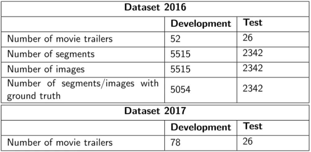
Dataset 2016
Development Test
Number of movie trailers 52 26 Number of segments 5515 2342 Number of images 5515 2342 Number of segments/images with
ground truth 5054 2342
Dataset 2017
Development Test
Number of movie trailers 78 26
Table 3.1: Structure of 2016 and 2017 dataset
3.1.3 Ground truth
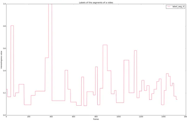
Ground truth annotations are provided for the images and for the video segments. The annotations were done by human assessors. For each sample, the interestingness value is given as 1 forinteresting and 0 fornot interesting. Additionally, a interestingness score is provided as a continuous value between 0 and 1. The rank of the image/segment within its movie trailer is also given.
Not all the images and segments have annotations because of the use of the adaptive square design method to annotate the data. This has to be taken into account for training the neural network since it requires both the input sample and its label. The number of segments and, consequently, the number of images for which annotations are provided, is the maximal number of segments which can be expressed as t =s2, where t is the number of segments and images with annotations in each video. E.g., for a video with 55 shots in total, only 49 = 72 shots and video frames, were annotated.
(a) [1, 1.0, 1] (b) [1, 0.327, 3] (c) [1, 0.729, 5] (d) [1, 1.0, 1] (e) [1, 0.238, 13]
(f) [0, 0.148, 80] (g) [0, 0.166, 57] (h) [0, 0.002, 77] (i) [0, 0.497, 11] (j) [0, 0.414, 13]
Figure 3.1: Example of interesting images (top row) and not interesting images (bottom row) with their [classification, interestingness value, and ranking] within its video respectively.
Figure 3.2: Ground truth labels of the segments of one video. Note that all the frames of one segment have the same label and the segments have different lengths.
3.2
Predicting Image Interestingness
The first subtask of the project is to predict image interestingness. To achieve this goal, a deep learning approach is explored.
3.2.1 Fine-tuning ResNet50
Fine-tuning means, given a pretrained model, modify it to approach a different problem. Since the pretrained model has its weights already calculated, the fine-tuned model will not start with random weights and this will help in the learning of the network. The model used for fine-tuning should be chosen according to what is the new problem to solve.
The model chosen for this task is theResNet50 [5]. ResNetis the Convolutinal Neural Network of Microsoft team that won the ILSRVC 20151 competition and surpassed the performance on the ImageNet dataset2. ResNet50 is one of the versions provided in the experiments of the
Microsoft team.
The Keras ResNet50 model3 has its weights pre-trained on ImageNet. Since it is pre-trained on images, we think that it will be easy to fine-tune and to obtain good results for predicting image interestingness. To fine-tune the network, different experiments have been performed by changing some parameters and analyzing the results for improvement.
The problem is approached as a classification problem, i.e. asoftmax activation is used at the last layer for predicting the probabilities for each class: 1 forinteresting and 0 fornot interesting
images.
3.2.1.1 Adding layers
The ResNet50 network 4 is a convolutional network formed by a feature extractor followed by a classifier with an output of 1000 dimensions. This output represents the probabilities for each one of the classes for the ImageNet classification 5. The model used for predicting image interestingness exchanges the last layer of the classifier (1000 dimensions) for our own classifier.
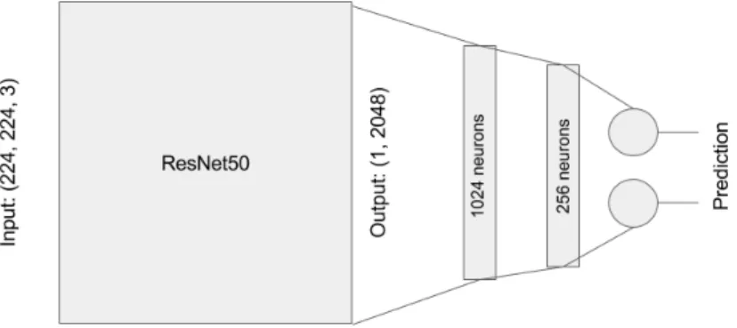
As commented before, we approach this problem as a classification task. Without the last layer, now theResNet50 network has 2048 dimensions as an output. With our classifier we want to obtain a prediction for each class: 1 for interesting, 0 for not interesting. To obtain this prediction a fully-connected layer with only two neurons and softmax activation is added after the 2048 dimensions layer ofResNet50.
With this architecture we obtain our first results. But since they still can be improved, more experiments are done adding more layers with different number of neurons in between the
ResNet50 and the two neuron output. Different learning rates are used to see the performance
1http://image-net.org/challenges/LSVRC/2015/ 2 http://image-net.org/explore 3https://keras.io/applications/#resnet50 4 http://ethereon.github.io/netscope/#/gist/db945b393d40bfa26006 5http://image-net.org/challenges/LSVRC/2015/browse-synsets
of the models.
Finally the architecture used for our next experiments consists of two fully-connected layers in between the ResNet50 and the two neuron output: first one with 1024 neurons and second one with 256 neurons. Figure 3.3 shows a schematic representation of the architecture.
Figure 3.3: Architecture of the network after adding layers.
3.2.1.2 Data augmentation
With the results obtained with the architecture of Figure 3.3 we observed that the model was learning in the training process but the validation curve was overfitting. We made a first hypothesis that this was happening because the dataset used was not big enough for the network to be able to learn.
For this reason we decide to augment our data to have more samples for training. We use theImage Data Generator 6 provided by Keras. This tool generates batches with real-time data augmentation. It also gives methods to upload the images from a directory, shuffle the samples, save the augmented images and much more.
TheImage Data Generator gives different options for processing the images. We just chose to augment our images with an horizontal flip. We did that because we wanted our network to see images that are interesting for human viewers. With the other options such as rotation, zoom or cropping the images had too much distortion.
We did some experiments with all the development data augmented, but we also tried to augment only images that are from the class Interesting. We did this due to the unbalanced dataset (see Section 3.2.1.4). By augmenting just the samples of classInteresting we could train the network with more samples of this class and make the data set less unbalanced, although still with morenot interesting samples thaninteresting
In some experiments we also augmented the dataset with height and width shifts, and with zoom besides the horizontal flip. We chose the following empirical numbers so the images have the minimum distortion but they can be seen as new samples:
• zoom range: 0.25
• height shift range: 0.25
• width shift range: 0.125
3.2.1.3 Dropout
After augmenting the dataset and having the architecture of Figure 3.3 our model was im-proving performance but the validation curve was still overfitting. We tried to see if our model would be better by adding dropout in between the layers.
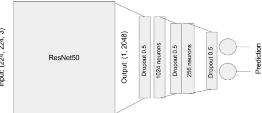
Overfitting sometimes happens because the model is too complex. Dropout consists in ran-domly setting a fraction of input units to 0 at each update during training time. Doing this we use the same model but we reduce complexity. In other words, not all neurons weights are updated each batch. The architecture used is represented in Figure 3.4. It is important to take into account that dropout only affects in the training process. In the testing the full model is used.
Figure 3.4: Architecture of the network after adding dropout.
3.2.1.4 Unbalanced classes
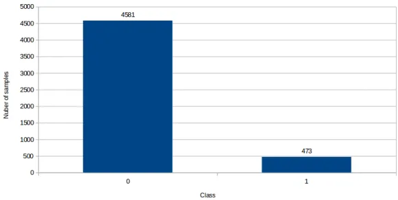
Another thing to be considered is that our dataset was unbalanced. We have approximately 90% of images of the classNo Interesting and 10% of images of the classInteresting (See Figure 3.5). Due to this, the network is seeing more samples of one class and this could bias the training and therefore the predictions.
One solution for dealing with unbalanced datasets is to give weights to the classes. This way the network uses this weights in the calculation of the loss function, giving more importance to the sample or classes that we want.
In our case, the weights for one classi were calculated using the following formula:
wi = 1 xi 1 n∗( 1 x1 + 1 x2... 1 xn) (3.1)
where wi is the weight of class i, xi is the number of samples of class i and n is the total number of classes.
Different separated experiments were run to deal with the unbalanced data:
1. Set manually the weights to 0.1 for class No Interesting and 0.9 for classInteresting due to the distribution of our dataset.
2. Reduce the No Interesting class to have the same number of samples as the Interesting
class and then augment both classes with the Image Data Generator from Keras. Class weights are not used.
3. Augment the Interesting class by flipping images horizontally (so we have double number of samples) and then reduce theNo Interesting class to have the same number of samples as the Interesting class. Class weights are not used.
4. Use the calculated weights with the formula 3.1 for the points 2. and 3. and repeat the experiments.
The experiments explained before were done first without the dropout (see section 3.2.1.3) and the results were analyzed. Then the dropout was added to some of the experiments with the best results to see if there was an improvement.
3.2.1.5 Train last layers ResNet50
The ResNet50 was trained with the ImageNet dataset, therefore the weights are already calculated to predict the 1000 classes of ImageNet. In the first experiments we are fine-tunning the network by adding new layers and calculating their weights without changing the weights of theResNet50 network. Later, the possibility of training the last inception blocks of theResNet50
network was explored.
To train the network, first our added layers were trained for 10 epochs. Next the last inception blocks were trained with our added layers for a number of epochs. The last inception blocks consist of the last 14 layers from the Keras model: they are the layers after the second last merging7.
With this experiments we want the hole network to be able to update the weights of more neurons and therefor try to improve the results. Despite this we observed that the results were more or less the same.
3.2.1.6 Classifier with SVM
Until now the classification problem has been done with a end-to-end deep learning network using an output of 2 neurons with softmax activation.
To be able to compare results with another type of classifier, a SVM is trained with the output feature vectors from the ResNet50. Different kernels are used to obtain the best results. After analyzing the results we can observe that the deep network architecture gives better results (See Chapter 4).
3.3
Predicting Video Interestingness
The second objective of the project is to predict video interestingness. To achieve this goal, a deep learning approach is also explored but with a different approach. A LSTM network will be trained with the features of the videos extracted from a 3D convolutional network.
As explained in Section 3.2, the problem is approached as a classification problem for predicting image interestingness. For predicting the interestingness of videos the problem is approached as a regression problem because we want a continuous value along all the segments of the video. Therefore, the label used for training the network is the interestingness level form the annotations instead of the binary classification label.
7
3.3.1 Extract features: C3D
Preprocess
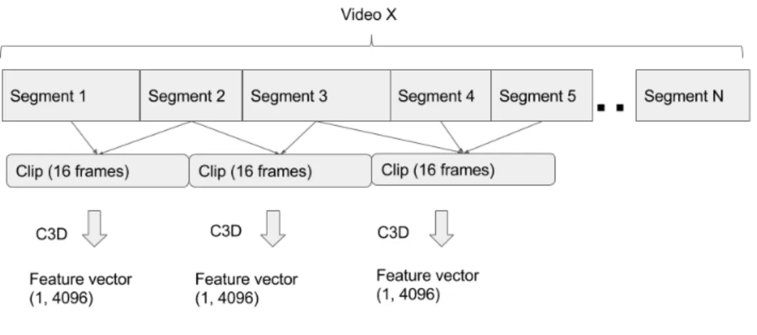
Before extracting the features of the videos with the 3D convolutional network, a preprocessing of the segments is needed because of the network input shape. The convolutional network extracts one feature vector for an input of a clip of 16 frames. Our video dataset is made of segments that have different number of frames with a minimum of 2 frames. To obtain clips of 16 frames, the segments that belong to the same movie trailer are put one after the other and grouped in clips of 16. If the number of frames of the movie trailer is not multiple of 16, the remaining frames are discarded.
At the end of this process, each movie trailer has the frames of the segments grouped in clips of 16 frames ready to extract the features.
Feature extraction
After the preprocessing of the video segments, the features of the clips of 16 frames are extracted using a 3D convolutional network. The model used for the network is the one used in [13] trained with theActivityNet dataset. The output feature vector has 4096 dimensions.
Figure 3.6: Preprocessing of the video segments for feature extraction with the C3D.
Label mapping
The labels provided in the ground truth are given for individual segments. The feature vector is extracted from a clip of 16 frames that may belong to one or more segments. Therefor a new label is needed for each feature vector before training the network.
The solution proposed is to take the weighted average of the labels of the segments in one clip taking into account the contribution of each segment in the clip as the number of frames.
Lci = Pk+N k WjSj Pk+N k Wj (3.2)
The weighted average is shown in the expression 3.2 where Lci is the label for clip i that is
the same as the label for the feature vector extracted from that clip. Wj is the number of frames (weight) of the segment j that is in clip ci. Sj is the interestingness score for that segment
(continuous value between 0 and 1). kis the first segment of the clip andN is the total number of segments in the clip. There is at least one segment in each clip.
The labels are back mapped once we obtain the prediction for each feature vector of a clip of 16 frames. The same approach as the label mapping from segments to feature vectors is done. The weighted average is computed with each of the labels of the clips that the segment belongs to. The weights are the number of frames that this segment has in each clip.
3.3.2 Fine-tuning LSTM network
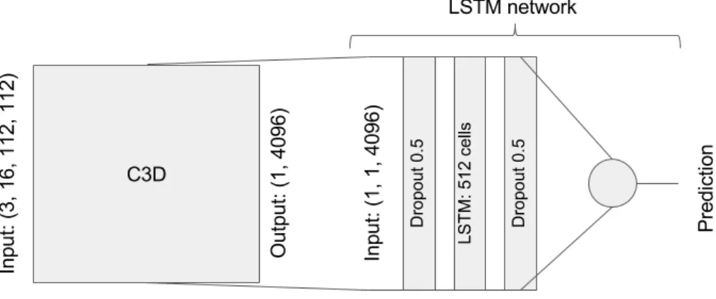
The model used for predicting video interestingness is a network that contains one Long Short Term Memory (LSTM) layer. LSTM networks are a special kind of recurrent neural network capable of learning long-term dependencies. One LSTM layer has some cells in it, and each cell has his own state. This state is the one that allows the network to learn time dependencies. The architecture of the pipeline is the one shown in Figure 3.7
As explained in the previous section, the input of the LSTM network are the features vectors extracted for each clip of 16 frames with the 3D convolutional network. Since we are dealing with video, we want the network to take into account the dependencies between consecutive feature vectors of one video.
The LSTM network from Montes et al [13] is the one used for training. It consists of 5 layers:
1. Abatch normalization layer that shifts inputs to zero-mean and unit variance. 2. Adropout regularization to prevent overfitting
3. The LSTM layer with 512 cells
4. Anotherdropout regularization
5. A fully-connected layer with 201 neurons for predicting each class probability
In the fine-tunning we first removed the last layer and instead we put a fully-connected layer with one neuron to predict the interestingness value. in Figure 3.7, the schematic of the network architecture is shown.
To train the network we have to make sure that features of different videos are not mixed, because this will make the LSTM learn time dependencies that we don’t want. To avoid that, all the features of one video are grouped and passed through the network for training. Next, the states of the cells are reseted and the same is done with the next video. Once the network has seen all the video samples, one epoch has finished and we start again the process for as many epoch we want.
After training and then predicting with the testset we obtained the same prediction for all the samples. This means that something was wrong. To solve this issue we took off the batch normalization layer. After this, the network was able to predict the interestingness value, but with a lower amplitude (see Figure 4.1). The hypothesis was that the network was learning to predict the average interestingness value instead of learning the interestingness time evolution.
Another approach that has not been explored but could be taken into account for future experiments is to input the LSTM with the raw pixels from the frames.
Chapter 4
Results
This chapter presents the results obtained with the experiments done with the methodology explained in Chapter 3.
4.1
Evaluation metric
The same evaluation metric is used for the predictions of image and video interestingness. The official evaluation metric used to compare the predictions with the ground truth is the Mean Average Precision (MAP) computed over all trailers, whereas average precision was to be computed on a per trailer basis, over all ranked images/segments. The computation of the MAP is made by a script provided by theMediaEval task organizers: the trec eval tool1. To compute the MAP a text file is needed with the classification value ofinteresting or not interesting along with a confidence value between 0 and 1 for each image and segment. As an output, the script provides the MAP of all the images and videos together with additional several other secondary metrics.
4.2
Baseline
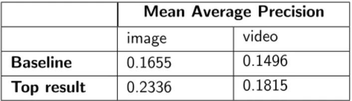
The baseline [2] for this project was generated by a random ranking run, i.e. samples were ranked randomly 5 times and the average MAP was taken. With this method, MediaEval ex-pects results to be better than just random ranking. The top result of the Predicting Media Interestingness task of 2016 is also taken into account.
Mean Average Precision
image video
Baseline 0.1655 0.1496
Top result 0.2336 0.1815
Table 4.1: Baseline and top results of 2016 for predicting image and video interestingness
4.3
Image interestingness results
The output of predicting image interestingness with the fine-tunned ResNet50 are the prob-abilities of being in each class: interesting or not interesting. To make the final classification a threshold has to be determined. E.g. if a image has a prediction of interesting: 0.6 and not
1
interesting: 0.4 and we use the threshold at 0.5 then the classification of that image will be ’1’ as interesting.
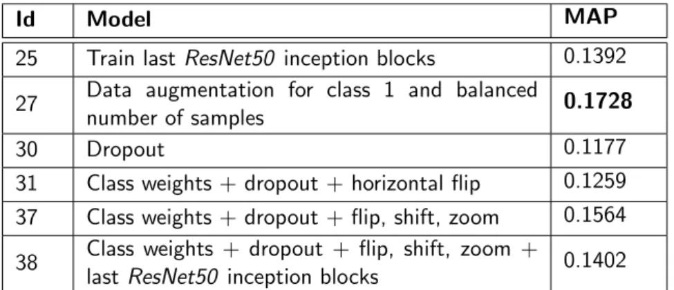
In Table 4.2 the MAP results of the best models are shown using a threshold of 0.5 for all the predictions.
Id Model MAP
25 Train last ResNet50 inception blocks 0.1392 27 Data augmentation for class 1 and balanced
number of samples 0.1728
30 Dropout 0.1177
31 Class weights + dropout + horizontal flip 0.1259 37 Class weights + dropout + flip, shift, zoom 0.1564
38 Class weights + dropout + flip, shift, zoom +
last ResNet50 inception blocks 0.1402
Table 4.2: Best MAP results of fine-tuning theResNet50 with 0.5 threshold
Another approach is to calculate a dynamic threshold for all the predictions. This method [2] was used by the organizers of the task to compute the ground truth. The method that they use to transform the interestingness values into binary decisions is the next one:
1. The interestingness values are ranked in increasing order and normalized between 0 and 1
2. The resulting curve is smoothed with a short averaging window, and the second derivative is computed
3. A threshold empirically set to 0.01 is applied on the second derivative to find the first point which value is above the threshold. This position corresponds to the limit between non interesting and interesting
In our case, the threshold used for the second derivative is set to 0, that is the point where the second derivative changes from negative to positive. After applying the dynamic threshold our MAP results improved, shown in Table 4.3
Id Threshold MAP 25 0.1577 0.1932 27 0.4875 0.1909 30 0.1572 0.2243 31 0.5066 0.2396 37 0.5295 0.2362 38 0.1336 0.1795
Table 4.3: Best MAP results of fine-tuning the ResNet50 with dynamic threshold
We can observe that the best results after using dynamic threshold were obtained with the models that had implemented class weights,dropout regularization and data augmentation.
Also some results were obtained using a SVM classifier to compare it to the end-to-end deep network architecture. The results using this type of classifier are shown in Table 4.4. Results show that the deep learning classifier with dynamic threshold gives better results than the SVM.
Id SVM Kernel MAP 40 linear 0.1392 41 rbf 0.1292 42 poly, grade 3 0.1425 43 poly, grade 4 0.1479 44 poly, grade 5 0.1471 46 sigmoid 0.1319
Table 4.4: MAP results using a SVM classifier
4.4
Video interestingness results
For the predicting video interestingness task, less results are obtained due to time permitting. Once all the videos were preprocessed and the network was trained the predictions are made. First, the prediction is made with a training video. Since the network has seen this video in the training process it should predict the output labels really good. In Figure 4.1 the labels from each feature vector corresponding to a clip of 16 frames are plotted along with the predictions made by the network. From the graph we can observe that the network is learning something about the peaks and valleys but the amplitude (interestingness value) is much lower.
Figure 4.1: Training labels (red) and predictions (green) of the feature vector labels for one video. x axes - feature vectors, y axes - interestingness value
With the predictions, the back label mapping is done (see Section 3.3.1) and the dynamic threshold is computed. In this case, the dynamic threshold is obtained from the second derivative of an approximated polynomial of order 3. This is done because the actual values have a high frequency component that affects the second derivative. The steps are almost the same:
1. The interestingness values are ranked in increasing order and normalized between 0 and 1
2. The resulting curve is approximated by a third order polynomial and the second derivative is computed
3. A threshold set to 0 is applied on the second derivative to find the first point which value is above the threshold (positive). This position corresponds to the limit between not interesting on the left and interesting on the right
On Figure 4.2 the procedure is shown for the predictions of one model. The top-left graph shows the normalized ranked interestingness values of all the video segments and the approxi-mated polynomial. The top-right graph shows also the approxiapproxi-mated polynomial. The bottom-left represents the first derivative and the bottom-right represents the second derivative of the approximated polynomial.
Since the threshold is set to 0 in the second derivative, that means that the threshold for the interestingness classification is in the change of concavity of the ranked values.
Figure 4.2: Graphs of the dynamic threshold computation.
Id MAP
65 0.1541
Table 4.5: Result for predicting video interestingness with the LSTM network
This result is above the baseline of0.1496. We can also compare the result with the Techni-color team [15] results since they used also deep learning architectures (see Section 2.1). With the LSTM architecture they got a MAP of0.1465.
Note also that the 3D convolutional network used for extracting the feature vectors was trained on the Sports1M 2 dataset. That means that the features extracted are good for predicting sports. This could bias the LSTM network while learning and after make predictions based on this features. One solution would be to use the features from the 3D convolutional network trained on the ActivityNet 3 dataset. In the Mediaeval task of 2017 this features are given but we have not used them because we decided to proceed with the other path. Another solution, but with more time and computational requirements, is to fine-tune the 3D convolutional network with our own dataset.
2http://cs.stanford.edu/people/karpathy/deepvideo/ 3
Chapter 5
Budget
This project has been developed using the resources provided by TU Wien, and as it is a comparative study, there are not maintenance costs.
Thus, the main costs of this projects comes from the salary of the researches and the time spent in it. It will be considered that my position has been as junior engineer, while the two professors who were advising me had a wage/hour of a senior engineer. I will consider that the total duration of the project was of 21 weeks, as depicted in the Gantt diagram in Figure 1.1.
Amount Wage/hour Dedication Total
Junior engineer 1 12,00 e/h 20 h/week 5,040 e Senior engineer 2 20,00 e/h 4 h/week 3,360 e
Total 8,400 e Table 5.1: Budget of the project
Chapter 6
Conclusions
The main objective of this project was to predict image and video interestingness. For both subtasks, some results are obtained and they are above the baseline. For this reason, I consider that the main goal of the thesis has been accomplished.
In the media community there is, to the best of our knowledge, no yet a perfect model for solving this task with high performance. Many models have been explored, and very few of them use a end-to-end deep learning architecture. Our solution has used a end-to-end deep learning architecture for predicting image and video interestingness.
For predicting image interestingness, fine tuning theResNet50 network has given good results. First we replaced the classifier of the ResNet50 for our own classifier. We realized that the new classifier was to simple so we made experiments by adding different number of layers with different number of neurons. Thanks to those experiments, we noticed that the network was learning but the validation curve was overfitting.
To prevent overfitting we first tried to augment the data set and after use the dropout
regularization. With this experiments, the network training improved but the predictions where still not as good as we wanted.
We realized that the training dataset had unbalanced classes and this was making the network to learn more about the not interesting class instead of the interesting class. To solve this problem we used class weights that helped the network to take into account both classes with the same importance.
All this changes improved the performance of our network. To explore more possibilities we also trained the last layers of theResNet50 network to see if the results improved. We observed that the results were more or less the same.
For predicting video interestingness, fine tuning the LSTM network has given results that are above the baseline. The challenging part of using LSTM network is how to train it making sure that it is learning time dependencies from the samples that you want. First, the video frames have to be grouped in a way to be able to extract the features. Next, this features are feed organized to the LSTM network. We realized that thebatch normalizationwas making our network predict always the same value, i.e the network was learning to predict an average interestingness value.
The predictions from both subtasks were a value between 0 and 1. If the threshold of 0.5 was used to classify the predictions in interesting or not interesting, the MAP was low. We learned that using a dynamic threshold the results improved in the image subtask. For the video subtask we directly used dynamic threshold. The dynamic threshold represents a ”jumping point” in the distribution of the ranked interestingness values.
As a future work, multi-modal (video and audio) approaches could be explored for the video subtask. Also, the C3D model used for extracting video features could be one trained with the
Chapter 7
Appendices
The code of the project can be found in the GitHub repository by the name of MediaInterest-ingness1. It has been fully developed in python using Keras with Tensorflow blackened.
In the repository, an unofficial sample application is provided. It is a simple telegram bot program that processes a image send by the user and returns the interestingness prediction.
1
Bibliography
[1] Jurandy Almeida. Unifesp at mediaeval 2016: Predicting media interestingness task.
[2] Claire-H´el`ene Demarty, Mats Sj¨oberg, Bogdan Ionescu, Thanh-Toan Do, Hanli Wang, Ngoc QK Duong, and Fr´ed´eric Lefebvre. Mediaeval 2016 predicting media interestingness task. InProc. of the MediaEval 2016 Workshop, Hilversum, Netherlands, 2016.
[3] Aykut Erdem Goksu Erdogan and Erkut Erdem. Hucvl at mediaeval 2016: Predicting interesting key frames with deep models.
[4] Michael Gygli, Helmut Grabner, Hayko Riemenschneider, Fabian Nater, and Luc Van Gool. The interestingness of images. In Proceedings of the IEEE International Conference on Computer Vision, pages 1633–1640, 2013.
[5] Kaiming He, Xiangyu Zhang, Shaoqing Ren, and Jian Sun. Deep residual learning for image recognition. InProceedings of the IEEE Conference on Computer Vision and Pattern Recognition, pages 770–778, 2016.
[6] Yu-Gang Jiang, Yanran Wang, Rui Feng, Xiangyang Xue, Yingbin Zheng, and Hanfang Yang. Understanding and predicting interestingness of videos. In AAAI, 2013.
[7] Harish Katti, Kwok Yang Bin, Chua Tat Seng, and Mohan Kankanhalli. Interestingness discrimination in images.
[8] Aditya Khosla, Atish Das Sarma, and Raffay Hamid. What makes an image popular? In
Proceedings of the 23rd international conference on World wide web, pages 867–876. ACM, 2014.
[9] Aditya Khosla, Akhil S Raju, Antonio Torralba, and Aude Oliva. Understanding and predict-ing image memorability at a large scale. InProceedings of the IEEE International Conference on Computer Vision, pages 2390–2398, 2015.
[10] Alex Krizhevsky, Ilya Sutskever, and Geoffrey E Hinton. Imagenet classification with deep convolutional neural networks. InAdvances in neural information processing systems, pages 1097–1105, 2012.
[11] Li-Jia Li, Hao Su, Li Fei-Fei, and Eric P Xing. Object bank: A high-level image representation for scene classification & semantic feature sparsification. InAdvances in neural information processing systems, pages 1378–1386, 2010.
[12] Luca Marchesotti, Naila Murray, and Florent Perronnin. Discovering beautiful attributes for aesthetic image analysis. International journal of computer vision, 113(3):246–266, 2015. [13] Alberto Montes, Amaia Salvador, Santiago Pascual, and Xavier Giro-i Nieto. Temporal
activity detection in untrimmed videos with recurrent neural networks. In1st NIPS Workshop on Large Scale Computer Vision Systems, December 2016.
[14] Soheil Rayatdoost and Mohammad Soleymani. Ranking images and videos on visual inter-estingness by visual sentiment features. In MediaEval, 2016.
[15] Yuesong Shen, Claire-H´el`ene Demarty, and Ngoc QK Duong. Technicolor@ mediaeval 2016 predicting media interestingness task. In MediaEval, 2016.
[16] Lorenzo Torresani, Martin Szummer, and Andrew Fitzgibbon. Efficient object category recognition using classemes. Computer Vision–ECCV 2010, pages 776–789, 2010.
[17] Baohan Xu13, Yanwei Fu23, and Yu-Gang Jiang13. Bigvid at mediaeval 2016: Predicting interestingness in images and videos.