A BRANCH PREDICTOR DIRECTED DATA CACHE PREFETCHER FOR OUT-OF-ORDER AND MULTICORE PROCESSORS
A Thesis by
PRABAL SHARMA
Submitted to the Office of Graduate Studies of Texas A&M University
in partial fulfillment of the requirements for the degree of MASTER OF SCIENCE
Chair of Committee, Paul Gratz Co-Chair of Committee, Jiang Hu Committee Member, Daniel Jimenez Head of Department, Chanan Singh
August 2013
Major Subject: Computer Engineering
ABSTRACT
Modern superscalar pipelines have tremendous capacity to consume the instruc-tion stream. This has been possible owing to improvements in process technology, technology scaling and microarchitectural design improvements that allow programs to speculate past control and data dependencies in the superscalar architecture. How-ever, the speed of the memory subsystem lags behind due to physical constraints in bringing in huge amounts of data to the processor core. Cache hierarchies have sub-dued the impact of this speed gap, however, there is much that can be still done in improving microarchitecture. Data prefetching techniques bring in memory content significantly before the instruction stream actually witnesses demand misses. How-ever, a majority of the techniques proposed so far depend upon an initial demand miss that initiates a stream of previously identified prefetches.
In this thesis, we propose a novel prefetching algorithm, which leverages branch prediction to facilitate deep memory system speculation. The branch predictor di-rected lookahead mechanism builds a speculative control flow path for the instruction stream about to be fetched by the main superscalar pipeline. Prefetches are gener-ated along this speculative path from a condensed representation of the memory instructions, leveraging register index based correlation. The technique integrates eloquently with the main pipeline’s branch predictor to filter out prefetches along invalid speculative paths. Impact of the prefetching scheme is analyzed using out-of-order model of the Gem5 cycle accurate simulator. Evaluation shows that on a set of 13 memory intensive SPEC CPU2006 benchmarks, our prefetching technique improves performance by an average of 5.6% over the baseline out-of-order processor.
DEDICATION
ACKNOWLEDGEMENTS
I would like to express my deep gratitude to my advisor, Dr. Paul Gratz for giving me an opportunity to work in the CAMSIN Group. His constant guidance and support always helped me move in the right direction in my research. I am really grateful to him for making my research experience a truly memorable one.
I would like to express my sincere thanks to Dr. Daniel Jimenez, for taking keen interest and giving his invaluable advice and suggestions during the course of this work. I would also like to thank Dr. Jiang Hu for agreeing to be on my thesis com-mittee and providing me valuable feedback and support.
A special thanks to the CAMSIN members who have worked with me on this, David Kadjo and Jinchun Kim. This work wouldnt have been possible without their valuable inputs and support.
My time at Texas A&M University was made enjoyable in large part due to many friends that became a part of my life. I am grateful for the time spent with room-mates and friends.
I would also like to thank my family for their love, support and encouragement throughout my life, and for inspiring me to always reach for higher and better edu-cation.
TABLE OF CONTENTS Page ABSTRACT . . . ii DEDICATION . . . iii ACKNOWLEDGEMENTS . . . iv TABLE OF CONTENTS . . . v
LIST OF FIGURES . . . vii
LIST OF TABLES . . . ix 1. INTRODUCTION . . . 1 1.1 Thesis Statement . . . 3 1.2 Document Organization . . . 4 2. PROPOSED APPROACH . . . 5 2.1 Background . . . 5 2.2 Motivation . . . 8 3. PRIOR WORK . . . 11 3.1 Prefetching . . . 11
3.2 B-Fetch for In-order Processors . . . 13
4. DESIGN AND IMPLEMENTATION . . . 17
4.1 Overall System Architecture . . . 17
4.2 System Components . . . 23
4.2.1 Branch Trace Cache . . . 23
4.2.2 Path Confidence Estimator . . . 26
4.2.3 Memory History Table . . . 29
4.2.4 Generate Deque . . . 35
4.2.5 Prefetch Deque . . . 39
4.2.6 Prefetch Filtering . . . 40
5. EVALUATION . . . 52
5.1 Methodology . . . 52
5.2 Results and Analysis . . . 54
5.2.1 Lookahead Depth Distribution Analysis . . . 54
5.2.2 Hit Rate Analysis . . . 59
5.2.3 Load Distribution in Basic Blocks . . . 61
5.2.4 MSHR Fill Analysis . . . 63
5.2.5 Performance Impact . . . 64
5.3 Hardware Overhead . . . 66
6. FUTURE WORK . . . 68
6.1 Priority Based Prefetch . . . 68
6.2 Dynamic Prefetch Region Sizing . . . 68
6.3 Dynamic Cache Selection . . . 69
6.4 Better Branch Prediction . . . 69
6.5 Multi-banked Tables . . . 70
6.6 Adaptive Lookahead Depth Threshold . . . 71
6.7 Instruction Cache Prefetching . . . 71
7. CONCLUSION . . . 72
LIST OF FIGURES
FIGURE Page
2.1 Relation between Data Access Pattern and Control Flow . . . 5
2.2 Branch Directed Prefetching . . . 7
2.3 Code Segment from SPEC CPU2006 . . . 9
4.1 B-Fetch Pipeline for OoO Processor . . . 18
4.2 B-Fetch Pipeline Internals . . . 22
4.3 Branch Trace Cache Structure . . . 24
4.4 Control Flow Graph and filled Trace Cache State . . . 25
4.5 Lookahead Algorithm . . . 27
4.6 Composite Branch Confidence Estimator . . . 28
4.7 Memory History Table . . . 30
4.8 Filled Memory History Table . . . 31
4.9 Prefetch Address Calculation Algorithm . . . 33
4.10 Generate Deque . . . 36
4.11 Generate Deque Forwarding Algorithms . . . 38
4.12 Prefetch Deque . . . 39
4.13 Prefetch Filtering via Flush from Main Pipeline . . . 41
4.14 Prefetch Filtering via Retire from Main Pipeline . . . 42
4.15 Memory History Update Algorithm . . . 44
4.16 Table Update Algorithm - Initial State . . . 45
4.17 Table Update Algorithm - Final State . . . 47
4.19 Calculating GenerateOffset Value in Offset Mode . . . 50
5.1 Lookahead Depth Distribution for SPEC CPU2006 FP Benchmarks . 55 5.2 Lookahead Depth Distribution for SPEC CPU2006 INT Benchmarks 56 5.3 Lookahead State Distribution . . . 57
5.4 Branch Trace Cache Hit Rate . . . 60
5.5 Memory History Table Hit Rate . . . 61
5.6 Prefetches Issued per Basic Block . . . 62
5.7 MSHR Fill Count Distribution . . . 63
5.8 IPC of B-Fetch Compared to Baseline and Stride . . . 64
5.9 Prefetch Lifecycle . . . 65
LIST OF TABLES
TABLE Page
5.1 Target Microarchitecture Parameters . . . 53 5.2 Hardware Overhead . . . 67
1. INTRODUCTION
Microarchitectural improvements and advancements in technology scaling have steadily increased processor speeds over the past decode. All this improvement has affected two out of the three major instruction categories, namely, control and arith-metic. Control instructions have gained speed owing to improvements in branch direction prediction and indirect branch prediction. Arithmetic instructions have witnessed major gains owing to technology and microarchitecture improvement in general. However, one front that is still left inadequately addressed has been the memory instructions. Memory instructions use a heavy network of design elements, which includes caches, main memory, and the underlying interconnection network, and in some applications the secondary storage. Studies [1, 9, 10] show that memory access latency is becoming a serious bottleneck towards further increase in system performance.
In an effort to bridge the gap between processor and memory speeds, many im-provements in techniques aim to mask the adverse effect of these high latencies. There is significant spatial and temporal locality in applications owing to the design of programs in general. This led to significant research to find ways of exploiting this spatial and temporal locality of references using Caches [22] between the processor and memory. With the advent of multicore systems another level of caches was added to the hierarchy and problem now included communication between cores. Through all this advancement in research, the ideas of spatial and temporal locality still hold true. As long as they do so, it is possible to direct focus of microarchitecture in exploiting these trends in memory access behavior. Several designs have been
im-plemented to improve cache behavior in general, which include, cache replacement policies, lock-up free caches [13] etc. These advancements tend to either reduce the number of misses or the hit time. However, these techniques do not target the penal-ties associated with long latency misses. The adverse effect only increases if a level of the cache hierarchy does not satisfy the miss, which is when main memory comes into play. It usually ends up taking hundreds of clock cycles to access memory in case a block does not exist in one of the caches.
The most commonly used technique currently used to hide the processor-memory speed divide is out-of-order execution. Out-of-order processors allow the instruction stream to continue past memory misses as long as there are no true data dependencies and the instruction window still has the available capacity. In essence, out-of-order execution overlaps the period in which a miss is being serviced, with execution of actual instructions making use of the underutilized resources. It is, however, possi-ble that much of the application code has a huge number of true data dependencies. Presence of such dependencies in the application code cripples the out-of-order core and forces it to operate at the speed of in-order cores while consuming many times the power and energy.
Prefetching is a well known technique that speculates on the memory address requirements of the instruction stream that is yet to appear in the main pipeline [12, 20, 17, 25, 24]. It issues requests for memory significantly before the actual memory instruction in the instruction stream issues a demand request. As previ-ously discussed, the higher up in the cache hierarchy that a block is, the lesser the time taken by the processor to access that block. In essence, a prefetcher eliminates the requirement to wait for an access to the main memory by bringing cache lines
closer to the processor core, in the high levels of the memory hierarchy. It is the efficiency of the prefetching technique that decides how much of the cache ends up being polluted by these prefetches. If prefetches end up evicting useful cache lines, they needlessly make the processor wait for those cache lines to be brought into the higher levels of the hierarchy again. Then there is the problem of large number of prefetch requests using up bandwidth that could otherwise be used in servicing de-mand requests. It is therefore very important for the prefetching algorithm to not only be proactive but also accurate.
1.1 Thesis Statement
This thesis attempts to explore and develop an innovative microarchitecture that takes care of the aforementioned requirements in order to design a prefetcher that is not only light weight and practical, but also highly effective in generating prefetch requests using the method of deep path speculation. We propose to take advantage of the advancement in branch prediction research in order create a lookahead stream that accurately represents the most likely control flow behavior expected from the instruction stream about to be seen in the main pipeline. Subsequently, we make use of the predictability in address generation format of memory instructions by captur-ing source register indices used for the same, seen at previous instances of the basic block (at basic block entry points). We use runtime values of the register file at these source register indices, to prefetch for basic blocks speculated by the lookahead stream.
1.2 Document Organization
The remainder of this thesis is organized as follows. In section 2 we discuss the background and motivation of our proposed approach. In section 3, we discuss prior work in prefetching and contrast our approach in B-Fetch for out-of-order, from a previous study done for in-order processors. Section 4 describes the prefetcher architecture in detail and in section 5 we discuss our methodology and evaluation of results. Section 6 lists the improvements that could potentially provide better performance gains in our current microarchitecture and we conclude in Section 7.
2. PROPOSED APPROACH
2.1 Background
This section provides a general overview of the branch-directed prefetching system and also discusses the motivation behind the proposed approach. The way that programs are constructed can be mapped to a control flow graph as shown in figure 2.1. The right side of the diagram shows the C code and its equivalent assembly is mapped to a control flow graph for clearity of understanding. We see that the direction of the branch determines which basic block shall be executed. The taken path on the right leads to one of the load instructions and the not taken path leads to the other load instruction. If we can predict where the branch will take us, we can effectively have an idea of what load shall be in the basic block subsequently following a branch instruction. This subtle but important link between branch instructions and the subsequent loads that shall be prefetched, leads to the core idea of the B-Fetch prefetcher.
To find out the path that a branch instruction shall take we make use of the branch predictor and the branch target buffer to guess the direction and the target basic block of branch instructions. On deciding upon a direction it is easy enough to find the link between a branch and the subsequent memory instructions seen in the linked basic block. The method thus described constitutes lookahead down one block.
Now that it is understood how to handle on basic block, our intention is to do so across multiple basic blocks, so as to create a path, for which, branches form the links until we reach to the end of the path. We make use of a branch trace cache structure to maintain a notion of what branch shall follow the current branch. The next branch information is used to index into the branch predictor and branch target buffer to dynamically determine the path in which the branch shall take us. However, it is not enough just to have a notion of where the branch predictor is taking us. We also need to be aware of certainties in going down a path. This notion of certainty is captured using a path confidence estimate. Path confidence is simply the cumulative confidence seen across all the branches that constitute a lookahead. The cumulative value is found by multiplying individual branch confidence values for branches that are part of the lookahead path. Hence, a low confidence branch tends to affect the path confidence estimate to great degree. The figure 2.2 gives the entirety of the B-Fetch algorithm in a very concise form.
Figure 2.2: Branch Directed Prefetching
The lookahead engine operates at the granularity of basic blocks and we are re-quired to lookup the value of path confidence estimate at each branch. If it is realized that the path confidence is not high enough, the lookahead engine stalls. It again resumes only when the path confidence estimates are high enough. Once the path confidence estimate is high, prefetches are issued for basic block that the branch leads to. It is then determined whether the lookahead engine has reached its maximum lookahead depth capacity. If it has, again, the lookahead engine is stalled. In case
that it is not, the lookahead engine move ahead and repeats the same process for the next branch.
2.2 Motivation
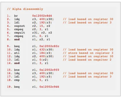
We now refer to figure 2.3. We see that there are three basic blocks in the code segment. In order to support the lookahead mechanism, the branches at entry points to these basic blocks need to be stored in a cache. This cache should essentially fa-cilitate lookaheads at the basic block granularity. We therefore, create a structure we term the branch trace cache to establish links between a branch instruction (en-try point of basic block), and the one that follows it in a particular direction, and with given target. Such an arrangement is needed since branches going to different directions (taken, not taken) and targets (indirect branches) may lead to different subsequent branch instructions.
Many of the loads are based on only a few register indexes. The link between branches and loads in the basic block is established using the source register indices that are used to create load addresses in the basic block. In the figure 2.3, these are register indices 30, 3, and 2. We link these source register indices to the correspond-ing branches that begin the basic block (entry points). This is done in a separate structure called the memory history table. The memory history table keeps track of the loads that exist in the basic block and links them to the corresponding branch instructions that lead to those basic blocks.
Figure 2.3: Code Segment from SPEC CPU2006
In this way, we keep a track of not only the path that branch instructions form, but also the loads that constitute those branch instructions.
Another aspect that needs to be discussed in this section is the actual calcula-tion of prefetch addresses. It is not enough to record the register indices that form the load. In the main pipeline, addresses are created by reading values for source registers of loads from the architectural register file. For the lookahead process, we need to access a more up to date runtime register file values when creating these addresses, since the register values would be stale if they were read from the archi-tectural register file. A separate register file structure updated at runtime by the dynamic execution core is maintained for this reason, which is called the execution register file in the remainder of this thesis.
It has been observed that there is considerable locality in the changes of register values across basic blocks and the change is highly correlated to fall within a 4-8 cache block spatial region size. This was the premise of a previous B-Fetch design for in-order cores [18]. To catch up to the changing register file values, we find the difference between the register file values read at the time of creating a prefetch ad-dress and the one seen in the commit stage. This offset is then used the next time prefetches are created to approximate the spatial variation in address values of the commit stage from the value of the register seen in the execution register file that reflects that state of the dynamic execution core.
Code based correlation is used in maintaining the branch trace cache and memory history table, because of which the storage requirement of these structures is not prohibitive. This is another factor that motivates our branch directed prefetcher design and makes it practical.
3. PRIOR WORK
This section discusses the work that is done in prefetching which relates to the field of study of this thesis. We first explore other approaches to prefetching and related topics. We then discuss work that bears passing resemblance to the ideas discussed in this thesis. The subsequent section we compare our work with a prior work done of B-Fetch for in-order processors [18].
3.1 Prefetching
Since the time that prefetching techniques have been explored, several attemps were made to support the design in this task. Earlier work focussed on changing the ISA. This method of prefetching used a totally different abstraction level to embody the idea of prefetching and has been discussed in [4], [15], and [26]. In its sim-plest form hardware prefetching was introduced in [21] in the form of the Sequential Prefetcher which prefeched caches lines successively following the cache block address that resulted in a demand miss. A Stride prefetcher [2] monitors demand misses and finds a pattern of repetitive behavior in the form of strides. Strides usually are a result of loop behavior in code. Content directed prefetcher [6] examines the content of the cache lines to find out if the words resemble a valid memory address and if so, prefetches for those addresses. In an extension to this work [8] hints are taken from the compiler in the form of ISA modifications to decide which of the addresses created with the CDP algorithm shall prove to be useful.
Another body of work related to pre-executing instructions speculatively with the hope that some of them might lead to memory instructions being correctly executed.
Such execution typically follows a demand miss leading to a long latency memory operation and is termed runahead prefetching [7]. An out-of-order version of this runahead mechanism [16] was proposed by Mutlu et al.
Spatial Memory Streaming [24] introduced one of the most practical prefetcher designs. It makes use of code-based correlation and takes advantage of locality (spa-tial) over a spatial region. As memory accesses are made the SMS prefetcher records patterns of accesses over a spatial region and encodes them in a bit vector. Once done they are then stored in a table. The prefetcher recognizes a pattern based on the first miss to a spatial region. This makes the prefetcher accurate but also renders the prefetcher dependent of witnessing misses in the data access stream which is a po-tential issue. As an extension of the SMS idea, to popo-tentially leverage performance previously lost as a result of waiting for misses to trigger prefetches, the STEMS prefetcher [23] was introduced. It took into account temporary characteristics of accesses to spatial regions and regenerated an entire stream of prefetches much more effectively compared to SMS. However, it incurred excessive hardware (of the order of 2 megabytes vs. roughly 33 kilobytes for SMS) for a 3% improvement in performance.
Branch Directed Prefetching techniques have been attempted in the past as well. The earliest work [14] proposes extending the branch target buffer to include a previ-ous address field, a stride field and metadata to manage state of the activating stride. The idea is to issue stride based prefetches while accessing the branch predictor and branch target buffer to go down a speculative path. A much more advanced work on the Tango Prefetcher [19] is an enhancement to the solution by Chen et. al.[5]. In this Tango prefetcher, dedicated tables are used to store the state of strides in a basic block while a lookahead mechanism attempts to predict branches at the rate
of one per clock cycle. This was done so as to issue prefetches way in advance before the superscalar processor would get to see actual loads from the instruction stream.
3.2 B-Fetch for In-order Processors
Our work is inspired by and is an extension to the previous work done by Panda et al. [18]. The previous work was predominantly a solution for in-order processors. We explore the differences and contrast the design of the two prefetchers here. We also discuss how the problem statement is different for the previous and the proposed B-Fetch design.
Design functionality is met by constructing a 4-stage pipeline that runs parallel to the main out-of-order pipeline. The broad goals considered while constructing this auxiliary pipeline (hereon called the B-fetch pipeline) were the ability to achieve very deep lookaheads across branches, to capture a subsequent amount of memory instructions within basic blocks, and to seamlessly be able to switch between loop and offset mode while generating memory addresses.
The new pipeline explores feasible ways to tackle problems in a previous version of the B-fetch pipeline for in-order systems that resulted because of certain design constraints that were sufficient for in-order systems but fall short for an out-of-order system which is the subject of this thesis. The following text explores these restrictions and why they need redesign.
1. Limited lookahead depths
Lookahead limit was restricted to a depth of around four basic blocks in B-fetch for in-order systems. This did not inhibit performance in such a system since
the rate of instruction consumption in in-order systems is relatively flat. Not only do they consume instructions one at a time but also end up stalling on misses a substantial number of times. For an out-of-order system instructions are essentially consumed at a very high rate, firstly because of its ability to ex-ecute instructions while bypassing anti and output dependences and secondly because of its wide construction and capacity to have more an a single instruc-tion in each of the pipeline stages. Such a consumpinstruc-tion hungry system can only benefit from lookaheads that are done way in advance of when the actual instruction even enters the main out-of-order pipeline. That can be made pos-sible only if lookahead stage is way ahead in speculating relative to the fetch stage. This would imply being at least twice as deep as the four basic block depth.
2. Lack of effective prefetch filtering
The previously explored in-order design of B-fetch had the tendency to some-times use excessive bandwidth. Once prefetches were let loose into the prefetch queue, there was essentially no way of retracting them in case it was realized later that the branch at some stage during the lookahead had been mispre-dicted. This may well have been a minor issue with for in-order systems, how-ever, for the very deep lookaheads that our design aims of achieving it would be very harmful if a lot of incorrect prefetches clog up the prefetch queue. Not only would this delay the issue of correct prefetch requests from being launched to the cache, but it would also be detrimental to overall system because of cache pollution. Especially if the L1 Data cache has a simply LRU policy there is more chance of a useful block being evicted to pull in prefetches. Our design aims at combating this menace by handling prefetches before and after
gen-eration much the same way as histories are managed in the branch predictor. Once it is realized that a lookahead was down a mispredicted path fetch over-rides lookahead and forces a flush to pervasively remove any prefetches that have already been or that may be created because of deep speculation along that incorrect path.
3. Insufficient load coverage
For the in-order B-fetch design had a maximum of five loads that could be allocated to the branch register table. Each entry had five units to support identification of five loads per basic block. This was based on profiling data collected that showed a majority of basic blocks has as many loads. However, without too much overhead our new design is able to pull in multiple loads for a register index into just one unit. This is possible because of a newly proposed compact and dense representation of loads based off of a particular register index. Also our design makes sure that loads after register redefinition are actually allocated new entries since their behavior is inherently different from previous loads off the same index after being modified to an arbitrary address.
4. Overbearing Bandwidth usage
The previous design begin modeled on an in-order core did not have a limitation as far as bandwidth availability is concerned. Because the density of loads being seen by the in-order execution unit is very less they lay less stress on the memory subsystem leaving substantial bandwidth available for making prefetch requests. Hence it was possible for the previous design to prefetch a band of cache lines termed a spatial region of eight contiguous cache lines. The dynamics of the game completely change when we talk about doing such a
thing for out-of-order systems. These systems are inherently fast consumers of instructions, be they memory or arithmetic or branch. As such because multiple loads can be outstanding at a moment, there is considerable usage of MSHR to hold outstanding requests while missed loads are being allowed to bypass. Prefetching a spatial region, intuitively, does not seem the best choice option since it would take up a large number of MSHR and bus bandwidth as a result. It is therefore a much wiser approach to restrict prefetching to a one cache line granularity or something that is less restrictive of the MSHRs and the bus bandwidth and that does not choke the load store unit of the main pipeline. Our design is restricted prefetching a single cache line.
5. The Multicore dilemma
Similar to the restrictions discussed above multicore systems is a different prob-lem in itself. A multicore system is much more bandwidth limited and does not play well to high demand in memory subsystem. A high prefetch rate in component cores lay stress to not only their L1 Data caches but also to the L2 cache. As such, having inaccurate prefetches flood the L2 cache adversely affects throughput of the multicore system. With high bandwidth demand comes the problem of energy wastage. Our designs tries to limit the scope of this problem with its filtering and stalling schemes, which limits the MSHR usage by prefetches and hence the demand for the subsystem resources.
4. DESIGN AND IMPLEMENTATION
We discuss the overall design and implementation of our proposed B-Fetch pipeline in this section.
4.1 Overall System Architecture
The types of instructions in the instruction stream are varied among branch, memory, and arithmetic types that produce the desired output of a program. Arith-metic instructions are typically fed input through load instructions that brings in data from lower levels of the memory hierarchy until they occupy state in the fastest storage structure possible, which is the register file. The time that it takes to bring in inputs to the program from down the memory hierarchy is a major contributor to the execution time of a program. Since long, even though the speed of process-ing arithmetic instructions has increased considerably, the speed at which input are brought in from the slower storage medium has not increased proportionately. The search for an answer to this problem has now fallen to microarchitects. Prefetch-ing attempts to bridge the gap between rate of delivery of inputs to the core from lower levels of the hierarchy and the rate at which arithmetic instructions consume these inputs to produce outputs. A processor pipeline proceeds every clock cycle at granularity of individual instructions. The intention behind B-fetch pipeline is to mark out the variable latency load instructions and store them in a structure that is representative of their behavior in the actual processor pipeline. In a sense B-fetch traces control flow in the form of branch instructions previously encountered in the main pipeline and attempts to pre-execute load instructions previously encountered along that control path. Because of its imitation of the main pipeline the B-fetch
pipeline is constructed somewhat similar to the main processor pipeline.
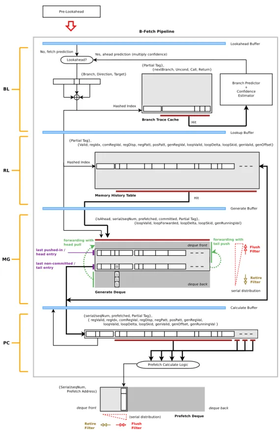
Figure 4.1: B-Fetch Pipeline for OoO Processor
Each of the B-fetch pipeline stages in figure 4.1 are discussed below. 1. Branch Lookahead Stage
Much like the fetch stage of the main pipeline branch lookahead functions with the support of a trace of previously encountered branches. This trace is stored in a structure called the Branch Trace Cache. The branch trace cache paves the way ahead for B-fetch pipeline at the granularity of basic blocks. It is a terse representation of all the branch instructions recently encountered
the instruction stream. When designing such a lookahead mechanism it is important to keep in mind that the directional support provided by the branch predictor is not infallible. Branch prediction is a speculative technique, in that, the speculation is not always correct. Hence a confidence estimator is used along with the lookahead mechanism that stops the lookahead from going down too deep along a speculative path.
2. Register Lookup Stage
Once it is known that the program flow will take a certain path in the future, a list of all the loads that were last seen down that path needs to be looked up. This lookup is of information about which registers constituted loads in a basic block. It is observed that there are typically not too many loads in repeating basic blocks. However, the design needs to have sufficient coverage so as to not overlook important loads that might block the main pipeline because of demand misses. Our design uses a very dense representation to capture the most common cases that arise as a result of loads distributed by the compiler in various forms within basic blocks. This representation of loads within basic blocks is captured in a structure called the Memory History Table that is part of this stage. It should be noted that not all basic blocks have loads. When committing branch traces in the lookahead stage above, it is required to have opening branch of every basic block in the trace cache. However, once the opening branch identity is propagated down the pipeline stage to the register lookup stage there might be a miss in the memory history table owing to the absence of loads in that basic block. Of course there also cases where aliasing knocks off entries that might actually be useful.
Once we have the knowledge of what loads are present in a basic block it is only a matter of unpacking the information present in the compressed rep-resentation to generate effective addresses that are dumped into the prefetch queue. However, there is a pitfall in how this creation of effective addresses is managed. We need to be able to propagate enough metadata into the prefetch deque to be able to wipe out prefetching once it recognized that they were down an incorrectly predicted lookahead path. Also it is not practically possible to create all prefetch addresses at once and push them onto the prefetch queue since that would require having a huge amount of write ports into the prefetch queue. In our highly dense design there is also the issue that each register unit defined within an MHT table entry needs to be decoded and address produced one after the other. Hence, a stage is required where entries are buffered into a deque structure once they are read from the MHT. Further, we reduce the overhead of loop maintenance by overloading this deque structure with the ca-pacity to forward running effective address values once it is recognized that a unit exhibits looping behavior.
4. Prefetch Calculate Stage
Once mode has been set and the required forwarding done, prefetches need to be calculated. Unlike previous B-fetch design for in-order core, address calculation cannot be done instantaneously within a single clock cycle. The problem mainly arises because of the densely encoded bits representing nega-tive and posinega-tive spatial locations around the (first) basic loads based off of a register index. The pattern needs to be decoded and related addresses need to be generated, sequentially unsetting the bit patterns in the process to mark that addresses corresponding to them have been created and pushed into the
prefetch deque. Because there are five units within an entry it can be possi-ble to put addresses into the prefetch deque from more than one such units at a time to parallelize the consumption of generate deque entries and speed up the calculate stage. However, that would not gain much since the prefetch deque addresses have only one port to make requests to the L2 cache limiting consumption of addresses to a maximum of one per clock cycle.
We shall now summarize the working of the B-Fetch pipeline’s pre-lookahead stage and thereafter lead the discussion toward exploring the technical design of each individual component involved in the various auxiliary pipeline stages.
As can be seen if figure 4.2 before the main pipeline there is a pre-lookahead stage. This stage is essentially a part of the fetch stage of the main pipeline. The func-tion of this stage to synchronize the events that are seen in the main pipeline with the auxiliary pipeline. Whenever a branch retires in the main pipeline the branch predictor of the main pipeline receives information about the retired branch. This allows the speculative history to be retired by writing its state onto the main branch predictor structures. This is how the retire signal integrates with the branch predic-tor. The B-Fetch pipeline simply borrows these signals and uses them to update its structures in the all the pipeline stages. These include the B-Fetch pipeline buffers, the generate deque, and the prefetch deque. Another signal that is borrowed from fetch stage’s communication with the branch predictor is the flush signal. Typically when there speculation proceeds down a path that is proved to be incorrect, all the state created because of that speculation is treated as begin useless and needs to be removed. The same thing needs to be done with the above mentioned structural components of the B-Fetch pipeline as well.
Technically, the prefetch deque is part of the L1 data cache, but because the B-Fetch pipeline needs to write content directly onto the deque structure and also flush/retire based on signals from the main pipeline, this structure is shared with between these two components i.e. Prefetch Calculate stage and the L1 data cache.
4.2 System Components
We shall now go through descriptions of each component used in the stages of the B-fetch pipeline. All the hardware structures are important in realizing an accurate and flexible branch directed prefetching scheme.
4.2.1 Branch Trace Cache
Every program has control nodes that block the flow of instructions in either one direction or the other. These branches, which are handled in the main pipeline by a branch execution unit, may also be speculated using a branch predictor. However, speculation itself does not form a good source of updating a trace cache structure. We therefore make use of branch commits to update the branch trace cache. The branch trace cache forms a series of links in the program control flow marked by branch instructions.
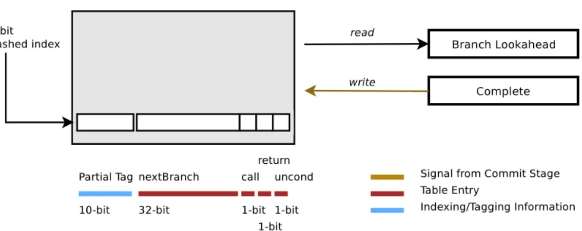
Figure 4.3: Branch Trace Cache Structure
An entry in the branch trace cache (shown in figure 4.3) is indexed by the current branch information, viz. its program counter, direction, and the target. It is im-portant to note here that different from in-order design for B-fetch, our design also uses target to generate branch trace cache index. Doing so inherently takes care of indirect branches. Hence, a branch that is predicted taken may land up executing instructions from different targets and each will have a different closing branch. So, once the branch trace cache is indexed as described it yields the branch that follows the current branch. This next branch is then fed to the branch predictor to deter-mine its target and direction, which then used to index the trace cache again to see if a valid path forward, exists for this branch. In this way, the branch trace cache structure helps guide lookahead stage forward and the branch predictor and target buffer help maneuver it in the right direction.
We now illustrate how the branch trace cache structure gets filled up using a control flow graph as the input. Figure 4.4 shows the example that we discuss
here. The control flow graph starts off with Branch 1 being the first encountered branch. When the commit stage first sees this branch it loads the branch address, the direction, and the target of this branch onto the last committed branch buffer (LCB). When the next branch following this branch retires, the LCB buffer shall be replace. Before that is done an entry is created whose index is decided by the current contents of the LCB buffer. A partial tag is inserted for semantic correctness. What the entry contains is the detail of the address of the next branch i.e. its address, and meta information required by the branch predictor, such as whether the branch is a call, a return, or an unconditional branch.
In this way an entry gets created in the branch trace cache. Following the taken path to basic block 3 (the target), the next branch is the Branch, which is an uncon-ditional branch and is illustrated as so in the figure 4.4. It is to be noted that the branch trace cache will have links for only the branches that have been seen by the commit stage of the main pipeline. That is to say that only the dynamic instruction stream gets to decide what is loaded onto the branch trace cache, not the static layout or the physical placement of code in the stream.
4.2.2 Path Confidence Estimator
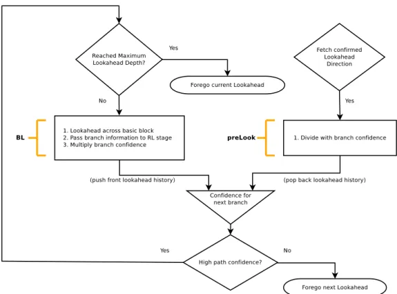
While looking ahead at the granularity of basic blocks it is not always wise to trust the prediction of the branch predictor. Lookahead down the incorrect path lead to incorrect address being prefetched. This can easily lead to cache pollution in the L1 data cache. It is therefore a very important requirement of the B-fetch design to have an estimation of the confidence of the path down which the lookahead engine is creating prefetch candidates. Once confidence falls below a certain preset threshold lookahead mechanism stalls to wait for the confidence to improve. Out B-fetch design has preset confidence thresholds for each level of depth of lookahead. More details can be found in figure 4.5.
The confidence threshold is set to a relatively lower value at small depths. This is done because out-of-order pipelines consume instructions pretty quickly. Lookahead always needs to be a certain number of basic blocks beyond what the main pipeline is executing. The situation is entirely different from in-order cores where every cache miss ends up stalling the main pipeline.
Figure 4.5: Lookahead Algorithm
We shall now discuss some of the technical details about the branch confidence es-timator design. The branch confidence eses-timator design is approximately a 2 kilobyte structure that uses the tournament predictor’s local and global history components to index into a two separate tables that contain confidence counters. The design has been inspired by Jimenez et. al. [11] that computes confidence as sum of the JRS up/down counters and self-counters salvaged from the tournament predictor itself. Local history is used to index a 1024 entry structure that has 5-bit confidence value for each of the histories. In the case the prediction matches the final outcome of the branch, the counter is incremented. However, in the situation that the prediction does not match the final outcome the whole counter value is right shifted i.e. divided by two. In this way, the counter remains more sensitive to misprediction than to
a correct prediction and is not easily biased by the high predictability of branches in the instruction stream. The second table is index using global history and has 4096 entries of 3-bit each. On correct prediction the confidence counter value is incre-ment and it is reset on a misprediction. The detailed algorithm is shown in figure 4.6.
The confidence values generated as a result of the prediction from the tournament value comprise of the values read from the 2-bit saturating counters of the tables. These values are also used as described in [11] to help compute the final confidence number value. Once the confidence number value has been found, it is simple enough to use this number to index into a number of ”confidence buckets”. In out design, the maximum confidence number (sum of confidence values from local/global confidence and predictor self counters) comes to be 44. These 44 buckets contain the confidence estimates for a classification of branches that index into a particular bucket.
Each of the 44 buckets keeps a track of how many predictions whose confidence number value indexed into a particular bucket proved to correct from the total num-ber of predictions made that indexed into that particular bucket. At regular intervals (such as a certain number of branches), the ratio of the total correct predictions to the total predictions that index into a bucket are computed. This fractional value is then used to estimate the confidence of individual branches. It is this fractional value that gets multiplied over consecutive lookaheads to determine the confidence of a path.
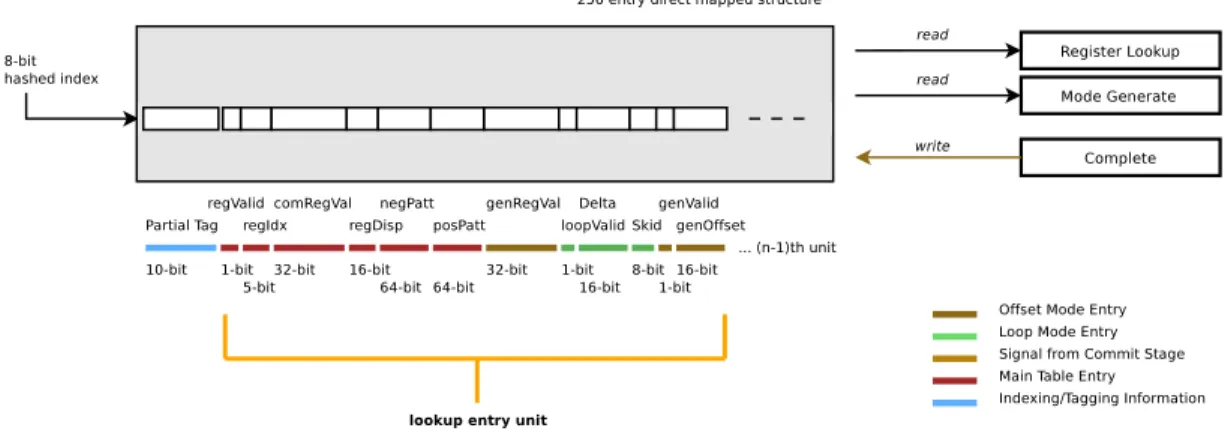
4.2.3 Memory History Table
Compaction of the loads seen in basic blocks resides in the MHT. Each entry (shown in figure 4.7) has associated metadata and a number of units that store in-formation specific to each basic load encountered within a basic block. From profiling it has been found that it is enough to have somewhere around five units to store indi-vidual basic loads information. Again entry and its associated units are updated at commit. The only exception to this is the register value picked up from the execution register file at the time of generation of prefetch addresses in the prefetch calculate stage of the B-fetch pipeline. There is a unit alias table associated with filling up of the entries into the MHT.
Figure 4.7: Memory History Table
A UAT (unit allocation table) takes care of cases where a register redefinition changes the register value that is used to create memory addresses. In such cases, a new entry linked to that register index gets created since the new load address may be completely unrelated to the initial loads and hence does not suffice as candidate for negative and positive pattern of unit previously assigned to the load based off of that register index.
Figure 4.8 represents the changes that occur in the MHT state. First time around the MHT is updated, at the commit stage when the instruction stream first gets seen by the out-of-order core. The second time around the instruction stream comes in from the fetch, lookahead mechanism gets activated and creates prefetches fol-lowed by writing in values of the execution register file that is used to create those prefetches. The instruction stream then goes to the commit stage and while com-mitting the state, realizes the difference between the actual register value used and the ones that were used to issue the prefetches.
Figure 4.8: Filled Memory History Table
The core idea behind B-Fetch shall be explained in brief in the following text. We continue the idea as explained above. We now intend to capture what the loads in a basic block look like. We also aim to capture the functioning of the two basic modes i.e. loop mode and offset mode.
1. Offset mode
There are three entries in the MHT that are used to support the offset mode i.e. generateRegVal, generateValid, and generateOffset. This is the mode that is activated by default in B-Fetch. This is actually the main core idea behind B-Fetch. What we intend to do is to create a snapshot of what the basic block looks like during the first go of the basic block in the commit stage of the main pipeline. This captures the displacement, register index and related entries as can be seen in figure 4.8 as is labeled in the figure. The next time around that the instruction stream gets seen, the value of the register index in the execution
register file (the register contents as they exist in the dynamic execution core) is picked up and recorded as the generateRegVal. The value is also marked as valid via generateRegValid. The B-Fetch prefetch engine then proceeds to create prefetch candidates for the memory address seen in the execution register file. The same instruction then moves onto the commit stage of the main pipeline where it reads the value of the architectural register file that was used to create the effective address for the load. This value is compared against the execution register file value that was used to create the prefetch in the first place. The difference between the two values is quantified in an entry called the generateOffset. Effectively, generateOffset is the difference by which the execution register value is running away (ahead or behind in terms of memory mapping) from the value which finally gets seen during the commit stage of the main pipeline. The next time that the instruction stream gets seen, the value of generateOffset gets added to the prefetch that gets created using the execution register file value. This is done in an attempt to get as near as possible to the value that will be seen in the commit stage in the architectural register file. A bit more detail is captured in figure 4.9.
Figure 4.9: Prefetch Address Calculation Algorithm
2. Loop mode
Another important aspect of the prefetch algorithm used in B-Fetch is the loop mode. It requires special fields to hold the value of dynamic change seen in memory references during each iteration of the loop. The fields are Delta, Skid and loopValid. The Delta value keeps track of the difference in commit stage effective address values of two consecutive iterations of the loop. Using the
last effective address value seen by the load and adding Delta on top of that value helps calculate value of the address for the next iteration of the loop that needs to be prefetched. The loop algorithm is validated each time a load is seen in the commit stage when it is not a new entry being created. Difference between the commit register value used to create the effective address the last time around is compared to the value of the commit register in the current commit. At a level beyond commit register values, it is confirmed that the delta’s are actually stable. For this the skid value is calculated as the difference between the originally existing delta in the memory history table entry and the one being calculated dynamically in the current commit state. If delta’s are constant the skid is zero and hence the entry qualifies for loop mode. Some over-provisioning has also been done, in that if the delta values are changing but the skid is constant we still classify the mht entry’s unit as being a valid candidate for loop mode. The loop mode algorithm comes into play in the generate deque structure before prefetches are actually created. Only when two instances of the same branch are seen in the generate deque structure, the old value of the generateRunningAddr is forwarded to the next value and delta/skid are added to create the memory address value that needs to be prefetched for that loop iteration.
The flowchart in Figure 4.9 shows how the entries in the MHT end up being used to create prefetch addresses in either one of the two modes - loop mode or the offset mode. The offset mode is enabled by default and loop mode comes into play when the generate deque has a entry that is valid for loop and was seen previously as part of the instruction window. More details on loop mode shall be explained in the section to follow.
4.2.4 Generate Deque
The third B-fetch pipeline stage called mode generate uses a deque structure called generate deque. The basic idea behind generate deque is to store information about loops that are inflight and to respond to squashes and updates from the main pipeline. Loops are recognized at the granularity of units of basic loads, not just MHT entries for the entire basic blocks. What this means is that out of the four units that can exist in the MHT entry, three units can be operating in offset mode, while one unit will be in loop mode. Recognizing such behavior within basic blocks where only on the load exhibits looping behavior is very important. In such a case, all entries were to be statically locked to loop mode behavior, there might be vari-ation in register value that could possibly be captured by the offset mode, which is based on dynamically reading the execution register file. We might miss out on the prefetch candidates that would otherwise be created in the offset mode. We shall now discuss the mechanism with which we implement looping behavior in our design.
Loops are identified in the commit stage, as discussed in the previous section. However, in B-Fetch as entries are read out of the MHT they are thrust onto the generate deque. When that is done the generate deque sifts between what units in what entries are classified as loops and if so, forwarding is done to take the current running values of memory addresses for the loop. Forwarding is possible in two ways in the generate deque. We discuss below why we need to account for two ways of forwarding and continue onto discussion about what exactly is forwarded.
Figure 4.10: Generate Deque
1. Forwarding via front pull
The forwarding algorithm of front pull is shown in the left side of figure 4.11. There might come a case when prefetches have been created for a basic block or its entry has been committed in the recent past. In such a case when a new instance of the same branch is pushed from the front of the generate deque 4.10, it needs to scan the deque associatively for a match. Once a match has been found and it is seen that the previous instance of that branch has either prefetched or has been retired, it is then probed whether the previous units of that branch entry were actually enabled for loops. Only when both, the new incoming branch and the old resident branch, instances of the same static branch have proven to be valid loops (via loopValid) do we actually forward
values for using front pull. Again, the pre-requisite of this technique is that the resident branch should either be an instance that has prefetched or one that has already committed. Another thing to keep in mind is that the associative search may give many matches. The match that is closest to the incoming branch being put in from the front of the deque is taken into account. This is done so that correction iteration of the loop is the one from which the incoming entry pulls its loop information. The forwarding in this case is driven by the head entry of the deque.
2. Forwarding via back push
This algorithm is shown on the right hand side of figure 4.11. This happens at the tail entry of the generate deque and the forwarding is driven by the tail entry of the generate deque. The tail entry of the deque is one which is the entry that is currently calculating its prefetch addresses in the prefetch calculate stage. Once it is done calculating all the prefetches it needs to the entry searches for a match from another instance of the same branch. Again, if there are multiple instances, the most recent one is taken in. The whole prioritization of associative search can be done with the help of a priority encoder circuitry. The intent of forwarding via back push is that when an entry is done creating prefetch candidates it should (with more priority than front pull) forward its value onto the next incoming basic block entry that is going to create its prefetch addresses. In the case the entry comes in later, after the calculate has already finished prefetching for the this basic block entry, the front pull algorithm can take care of handling the loops.
In this way, as described above, both the front pull and back push contribute to making sure that loops are handled correctly via forwarding and adding of address
values in the generate deque structure itself. No additional calculation is later re-quired when prefetches are calculated in the prefetch calculate stage since the running sum of address holds the next address that a loop needs to create for a particular unit.
Figure 4.11: Generate Deque Forwarding Algorithms
To sum up, once it is recognized that a unit in MHT entry is behaving as a loop its entry in the generate deque latches onto a running value of effective addresses be-ing generated at each loop iteration. This runnbe-ing value is then used is the prefetch calculate stage to handle creation of effective addresses for loops.
Another thing that needs to be discussed in context to generate deque (that also applies to prefetch deque in next section) is the process of filtering. Filtering is
brought out with the help of two predominant signals that are borrowed from the main pipeline, i.e. the flush and the retire signals. We shall discuss, more in detail, about filtering mechanisms in the next section once we develop an understanding of how prefetch deque works.
4.2.5 Prefetch Deque
This structure holds the prefetch addresses that created in the prefetch calculate stage and yet to be issues as a request. With such an aggressive lookahead mechanism it is important to be able to discard prefetches that have been created from deep lookaheads, once it is known that the fetch engine itself is being redirected. If that were not done, a vast amount of prefetches would still remain in the prefetch deque that really have not use and will just end up polluting the L1 data cache. The structure of prefetch deque is shown in figure 4.12.
All the address values that are created in the prefetch calculate stage are pushed onto the back of the prefetch deque. How these address values are created shall be explained in the following text. Once a value is brought to the Calculate Buffer from the generate deque structure, it is all set to create prefetch addresses. All the candi-dates are classified as being in offset mode unless the generate deque has a flag that tells this stage that a loop was identified and its value was subsequently forwarded. This is the loopForwarded bit of the calculate buffer. In case the offset mode is set, the current value of the execution register file is read and its corresponding address is created for prefetch using the sum of execution register file, displacement, and the offset previously discussed.
4.2.6 Prefetch Filtering
We shall now discuss the two methods of prefetch filtering that have been de-scribed as an integral part of the the generate deque and the prefetch deque. The prefetch filtering process not only takes place in these two structures but is also done in the buffers that drive each of the pipeline stages. Broadly speaking all those prefetches need to be filtered which have no connection to the future execution path and whose instruction stream is no longer part of the the main pipeline. What that means is that all the prefetches that are on a path that has been known to be incor-rect, they need to be flushed from the B-Fetch pipeline. Also, all prefetches whose loads have already issued demand requests to L1 data cache also have no place in the B-Fetch pipeline.
Figure 4.13 describes the algorithm for filtering the B-Fetch pipeline based on flush signals received from either the decode stage of the main pipeline or a flush
due to branch mispredict. In such a case, all the instructions that appear after the mispredicted instruction in the instruction stream - which may be part of the lookahead stream - need to be removed, since an edge in the control flow graph has been proven to have been speculated down the incorrect path. In the flowchart of figure 4.13 we drive the flush through each of the buffers of the auxiliary pipeline followed by the generate deque and then the prefetch deque. This ensures a clean sweep of incorrect state.
Figure 4.13: Prefetch Filtering via Flush from Main Pipeline
affects the branch prediction history structures. In branch predictors speculatiev histories are created as the speculation progresses one branch at a time. The main prediction history structures cannot be updated on speculation and hence, specula-tive local and global histories are maintained.
Prefetches are filtered both ways in the deque. First because of updates from commit, since they would already have been taken care of by the main pipeline. And second because of squashing due to branch mispredictions or exceptions. Filtering is triggered by squash and commit signal from the main pipeline.
Figure 4.14: Prefetch Filtering via Retire from Main Pipeline
Now, to discuss how retire signal affects the filtering process, we need to make sure the same mechanisms are installed for retire as are for flush. The only difference is
that retires take place of instructions that are older in the instruction stream, which means that we need to remove basic block entries in generate deque and prefetch deque from the other side of the deque than the one used by the flush signal. The motive behind using the retire signal is that we should get to creating prefetches which actually matter in the context that will show up in the future. Essentially, if prefetches were not generated for a basic block and all of its instructions have retired, they would very well have issued all their loads and got a response from the lower levels of the cache hierarchy. In such a case it better to have the prefetch calculate stage calculate prefetch addresses for a basic block that is about to show up in the future of the instruction stream. We see the concise algorithm in figure 4.14.
4.3 Working Example
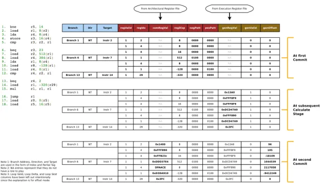
The working example illustrates how the the flowchart in figure 4.15 is used to update the MHT, the first and second time the commit sees the instruction stream.
Before starting with the working example we build a bit of background as to how we shall progress through this example. In figure 4.16 and figure 4.17 we update table state based on the context collected during retirement of individual instruc-tions in the commit stage of the main pipeline. The algorithm for the same has been presented in the form of a flowchar in figure 4.15. All the components that form an important part of the commit update process are displayed in figure 4.16. These include the branch trace cache, the memory history table, unit allocation ta-ble and the last committed branch buffer. To start with the description, we need to understand that we are building links between branches in the branch trace cache and gathering load context observed in basic blocks in the memory history table
entries. For the sake of simplicity this example only explains the offset mode. The loop mode working has been explained in previous sections and shall not form part of this discussion. For this reason the generate deque is also not an important aspect of this discussion and is not shown here. So as branches and load instructions retire they update B-Fetch context.
Figure 4.15: Memory History Update Algorithm
The first thing to update is the last committed branch buffer. This has infor-mation about the branch that was committed most recently and is used to create a
link between that branch and the branch the will next be retired in commit order. The initial and final state are shown in the relevant figures. Because all the branch instructions that have been encountered has simply committed with not taken direc-tion during this observed control flow they have only entries corresponding to that direction alone to create the links. There are certain special aspects of entry creation in the commit stage that we shall discuss in this example.
Figure 4.16: Table Update Algorithm - Initial State
The first thing to notice is that in the table entry for branch 1 there are two entries with register index 4. This is so because in instruction 3, the register at index 4 has been redefined. Because it has been redefined we need to create a new entry
for it, since the context has the possibility to jump to anywhere within the address space based on the content of the register at index 4 itself, which is used to create the address for that load. The second peculiarity is the entry for Branch 6. Both instructions 7 and 8 are loads based off of register at index 1 and since there is no redefinition, both these loads are squeezed onto one unit in the entry for branch 6. That has been made possible with the help of the negPatt field which is basically the relative displacement of the second load when compared to the first load based on that offset. It just so happens that in this example the second load off of register at index 7 is 2 cache blocks in away from the first load in the negative direction and hence we set the second bit of the negPatt to symbolize this relationship. Similary, loads at instructions 10 and 11 have this relationship but set the posPatt second bit. This basically compresses the entry and helps us store more loads from the basic blocks into a restrictive number of entries in the memory history table, which is four in our case.
Eventually, the table fills up and commit stage has gone through the code once. Figure 4.17 shows the final state once we go through the code in the figure. This state shall be used to create memory addresses for prefetch when the stream is seen next time around in the fetch stage of the pipeline.
Figure 4.17: Table Update Algorithm - Final State
To summarize, figure 4.16 shows all the components in the B-Fetch pipeline that are updated from the commit stage of the main pipeline. Once all the instructions have been committed, both the BTC and the MHT get the information about the instruction stream. This is illustrated in figure 4.17. This information then guides the lookahead mechanism in creating prefetch candidates that get issued to the L1D cache.
Figure 4.18: Post Prefetch Issue Memory History Table State
The next time around that the fetch stage sees this instruction stream, the looka-head stage gets activated. This link is established through the pre-lookalooka-head being integrated with the fetch stage of the pipeline. As this lookahead mechanism gets activated the instruction stream is no longer a driver. What drives the lookahead stream is the branch trace cache and the memory history table. the branch trace cache is indexed for first branch i.e. branch 1 to find which is the linked branch in the direction and with that particular target. Once that is known the current branch information is flown down the pipeline and linked branch is fed back to the branch trace cache to find the next link. As can been seen in the figure, the lookahead buffer, lookup buffer, generate buffer, and calculate buffer are shown in this figure 4.18. So
in the next cycle, MHT is accessed the the accessed entry flows down the pipe until it sees the calculate stage. When in the calculate stage, the prefetch addresses are created one per unit at a time. In special cases, where negPatt and posPatt are seen, they are processed in the next clock cycle which new entries are held back in the generate deque.
While this process happens, the algorithm used to create prefetch addresses is in offset mode. In this algorithm, the value of the execution register file is read and thereafter prefetch addresses are created. The value that is used to create the prefetches are recorded in the genRegVal field and its valid bit is set. This shall be consumed in the upcoming commit phase of this instruction stream.
To summarize, once prefetches have been issued, the MHT is updated with in-formation about what values were picked up from the execution register file while creating prefetch addresses. Once the prefetch addresses are known, they can be compared to the actual register values that get seen during the commit stage. This is shown in figure 4.18.
Figure 4.19: Calculating GenerateOffset Value in Offset Mode
At the second commit of the instruction stream, in values of effective addresses are observed. These need to be compared with the effective addresses that have been generated in the lookahead stage, to find out how different they were from the ones that calculate stage made. This is done along with retiring of individual instructions. As genValid is recognized to be set, the value of the genValid and invalidated. The generateOffset value is computed as the difference between the register value seen in the architectural register file and the one seen in the execution register file. The one seen in the execution register file was previously recorded in the genRegVal field. This gives us the difference between the dynamic execution core based value of effective address generated and the actual effective address as seen by the second commit.
So, now that the commit has seen the difference between the prefetch register value used and the commit register value used, the difference is computed as the Generate Offset. This offset shall be added the next time around the prefetch gets issued. The figure 4.19 only shows the offset mode. The loop mode is similar and hasn’t been discussed for brevity.
5. EVALUATION
In this section we lay emphasis on the evaluation of our design. We lay much stress on the internals of our microarchitecture, to build to the final results, going through statistics from each stage.
5.1 Methodology
Simulations were performed using Gem5 [3], a cycle accurate simulator . The ar-chitectural configuration is shown in Table 5.1. We model a 5-stage 20-deep pipeline out-of-order pipeline using the o3 pipeline model in Gem5. The pipeline is 2-wide which is comparable in configuration to most modern architectures in use today. The modelled memory uses the gem5 classic memory model. It is a two level cache hierarchy with a 64 kilobyte 4-way set associative L1 instruction cache, as well as data cache. The level 2 cache is 2 megabytes in size and 16-way set associate. The configuration of the memory model is such that memory accesses time for level 1 caches is 1 ns, while that for level 2 cache is 16 ns. The main memory takes 60 ns to service a request.
We run 13 of the memory intensive SPEC CPU2006 benchmarks, compiled for ALPHA ISA. The simulation runs in system emulation mode for SPEC benchmarks. Multicore simulations use PARSEC benchmarks in full system mode. Results pre-sented hereafter use around 2 billion instructions to gather simulation statistics with the reference input set.1
Table 5.1: Target Microarchitecture Parameters
Simulator Gem5 Simulator, ALPHA ISA, Full System Simulation / System Emulation Mode
Architecture O3 5-stage 20-deep Pipeline, 2-wide, 2 GHz Frequency
Branch Predictor Tournament Predictor
BTB 4096 entries
Register File Gem5 Simulator, 32 Integer Registers, 32 Floating-point Registers
ICache / DCache 64KB, 4-way set-associative cache, 64 Byte Line size, 1 ns access latency, 10 MSHRs, 3 Cache Ports L2Cache 2MB, 16-way set associative, 64 byte line size, 16 ns
access latency, 20MSHRs, 1 port
Memory 60 ns access Latency
The number of MSHRs plays a vital role here. The number of outstanding re-quests to the L1 data cache is dependent on the MSHRs available. Once a request is made to the L1 cache an MSHR gets allocated and is freed only when the request is serviced. it should be noted here that out of the 10 MSHRs, B-Fetch prefetcher is allowed to use up only a maximum of 70% of the capacity. Rest are always left for demand accesses.