AMELIA II: A Program for Missing Data

(1)

AMELIA II

: A Program for Missing Data

James Honaker, Gary King, and Matthew Blackwell

Version 1.7.4

December 5, 2015

1 Introduction

Missing data is a ubiquitous problem in social science data. Respondents do not answer every question, countries do not collect statistics every year, archives are incomplete, subjects drop out of panels. Most statistical analysis methods, however, assume the absence of missing data, and are only able to include observations for which every variable is measured. _Amelia_IIallows users to impute (“fill in” or rectan-gularize) incomplete data sets so that analyses which require complete observations can appropriately use all the information present in a dataset with missingness, and avoid the biases, inefficiencies, and incorrect uncertainty estimates that can result from dropping all partially observed observations from the analysis.

AmeliaIIperformsmultiple imputation, a general-purpose approach to data with

missing values. Multiple imputation has been shown to reduce bias and increase ef-ficiency compared to listwise deletion. Furthermore, ad-hoc methods of imputation, such as mean imputation, can lead to serious biases in variances and covariances. Unfortunately, creating multiple imputations can be a burdensome process due to the technical nature of algorithms involved. _Amelia provides users with a simple way to create and implement an imputation model, generate imputed datasets, and check its fit using diagnostics.

The _Amelia _II program goes several significant steps beyond the capabilities of the first version of _Amelia (Honaker, Joseph, King, Scheve and Singh., 1998-2002). For one, the bootstrap-based EMB algorithm included in _Amelia _II can impute many more variables, with many more observations, in much less time. The great simplicity and power of the EMB algorithm made it possible to write _Amelia _II so that it virtually never crashes — which to our knowledge makes it unique among all existing multiple imputation software — and is much faster than the alternatives too. _Amelia_II also has features to make valid and much more accurate imputations for cross-sectional, time-series, and time-series-cross-section data, and allows the incorporation of observation and data-matrix-cell level prior information. In addition to all of this,_Amelia_IIprovides many diagnostic functions that help users check the validity of their imputation model. This software implements the ideas developed in Honaker and King (2010).

2 What

_A

melia Does

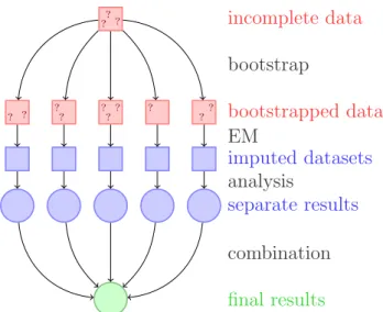
Multiple imputation involves imputing m values for each missing cell in your data matrix and creatingm“completed” data sets. Across these completed data sets, the observed values are the same, but the missing values are filled in with a distribution of imputations that reflect the uncertainty about the missing data. After imputation with _Amelia _II’s EMB algorithm, you can apply whatever statistical method you would have used if there had been no missing values to each of the m data sets, and use a simple procedure, described below, to combine the results1_{. Under normal}

circumstances, you only need to impute once and can then analyze the m imputed

1_{You can combine the results automatically by doing your data analyses within Zelig for R, or}

(4)

data sets as many times and for as many purposes as you wish. The advantage of

AmeliaIIis that it combines the comparative speed and ease-of-use of our algorithm

with the power of multiple imputation, to let you focus on your substantive research questions rather than spending time developing complex application-specific models for nonresponse in each new data set. Unless the rate of missingness is very high,

m= 5 (the program default) is probably adequate.

2.1 Assumptions

The imputation model in _Amelia _II assumes that the complete data (that is, both observed and unobserved) are multivariate normal. If we denote the (n×k) dataset asD (with observed part Dobs _{and unobserved part} _Dmis_{), then this assumption is}

D∼ Nk(µ,Σ), (1)

which states thatD has a multivariate normal distribution with mean vectorµand covariance matrix Σ. The multivariate normal distribution is often a crude approx-imation to the true distribution of the data, yet there is evidence that this model works as well as other, more complicated models even in the face of categorical or mixed data (see Schafer, 1997; Schafer and Olsen, 1998). Furthermore, transforma-tions of many types of variables can often make this normality assumption more plausible (see 4.4 for more information on how to implement this in _Amelia).

The essential problem of imputation is that we only observeDobs_{, not the entirety}

of D. In order to gain traction, we need to make the usual assumption in multiple imputation that the data are missing at random (MAR). This assumption means that the pattern of missingness only depends on the observed data Dobs_{, not the}

unobserved data Dmis. Let M to be the missingness matrix, with cells mij = 1 if

dij ∈Dmis andmij = 0 otherwise. Put simply,M is a matrix that indicates whether

or not a cell is missing in the data. With this, we can define the MAR assumption as

p(M|D) =p(M|Dobs). (2) Note that MAR includes the case when missing values are created randomly by, say, coin flips, but it also includes many more sophisticated missingness models. When missingness is not dependent on the data at all, we say that the data are missing

completely at random (MCAR). _Amelia requires both the multivariate normality

and the MAR assumption (or the simpler special case of MCAR). Note that the MAR assumption can be made more plausible by including additional variables in the dataset Din the imputation dataset than just those eventually envisioned to be used in the analysis model.

2.2 Algorithm

In multiple imputation, we are concerned with the complete-data parameters, θ = (µ,Σ). When writing down a model of the data, it is clear that our observed data is actually Dobs _and _M_{, the missingness matrix. Thus, the likelihood of our observed}

(5)

data isp(Dobs_{, M}_|_θ_{). Using the MAR assumption}2_{, we can break this up,}

p(Dobs, M|θ) = p(M|Dobs)p(Dobs|θ). (3) As we only care about inference on the complete data parameters, we can write the likelihood as

L(θ|Dobs)∝p(Dobs|θ), (4) which we can rewrite using the law of iterated expectations as

p(Dobs|θ) =

Z

p(D|θ)dDmis. (5)

With this likelihood and a flat prior onθ, we can see that the posterior is

p(θ|Dobs)∝p(Dobs|θ) =

Z

p(D|θ)dDmis. (6) The main computational difficulty in the analysis of incomplete data is taking draws from this posterior. The EM algorithm (Dempster, Laird and Rubin, 1977) is a simple computational approach to finding the mode of the posterior. Our EMB al-gorithm combines the classic EM alal-gorithm with a bootstrap approach to take draws from this posterior. For each draw, we bootstrap the data to simulate estimation uncertainty and then run the EM algorithm to find the mode of the posterior for the bootstrapped data, which gives us fundamental uncertainty too (see Honaker and King (2010) for details of the EMB algorithm).

Once we have draws of the posterior of the complete-data parameters, we make imputations by drawing values of Dmis _{from its distribution conditional on}_Dobs _and

the draws of θ, which is a linear regression with parameters that can be calculated directly from θ.

2.3 Analysis

In order to combine the results across m data sets, first decide on the quantity of interest to compute, such as a univariate mean, regression coefficient, predicted probability, or first difference. Then, the easiest way is to draw 1/msimulations ofq

from each of them data sets, combine them into one set ofm simulations, and then to use the standard simulation-based methods of interpretation common for single data sets (King, Tomz and Wittenberg, 2000).

Alternatively, you can combine directly and use as the multiple imputation esti-mate of this parameter, ¯q, the average of themseparate estimates,qj (j = 1, . . . , m):

¯ q = 1 m m X j=1 qj. (7)

2_{There is an additional assumption hidden here that}_M _{does not depend on the complete-data}

(6)

incomplete data ? ? ? ? ?? ? ? ?? ? ?? bootstrap bootstrapped data imputed datasets EM analysis separate results combination final results

Figure 1: A schematic of our approach to multiple imputation with the EMB algo-rithm.

The variance of the point estimate is the average of the estimated variances from

within each completed data set, plus the sample variance in the point estimates

across the data sets (multiplied by a factor that corrects for the bias because m <

∞). LetSE(qj)2 denote the estimated variance (squared standard error) of qj from

the data set j, and S_q2 = Σm_j₌₁(qj −q¯)2/(m−1) be the sample variance across the

m point estimates. The standard error of the multiple imputation point estimate is the square root of

SE(q)2 = 1 m m X j=1 SE(qj)2+Sq2(1 + 1/m). (8)

3 Versions of

_A

melia

Two versions of_Amelia_IIare available, each with its own advantages and drawbacks, but both of which use the same underlying code and algorithms. First, _Amelia _II exists as a package for the R statistical software package. Users can utilize their knowledge of theRlanguage to run_Amelia_IIat the command line or to create scripts that will run_Amelia_IIand preserve the commands for future use. Alternatively, you may prefer_Amelia_View, where an interactive Graphical User Interface (GUI) allows you to set options and run _Amelia without any knowledge of the R programming language.

Both versions of_Amelia _IIare available on the Windows, Mac OS X, and Linux platforms and _Amelia _II for R runs in any environment that R can. All versions of

Amelia require theR software, which is freely available athttp://www.r-project. org/.

Before installing _Amelia _II, you must have installed R version 2.1.0 or higher, which is freely available at http://www.r-project.org/.

(7)

3.1 Installation and Updates from R

To install the _Amelia package on any platform, simply type the following at the R

command prompt,

> install.packages("Amelia")

andRwill automatically install the package to your system from CRAN. If you wish to use the most current beta version of _Amelia feel free to install the test version,

> install.packages("Amelia", repos = "http://gking.harvard.edu")

In order to keep your copy of _Amelia completely up to date, you should use the command

> update.packages()

3.2 Installation in Windows of

_A

melia

_V

iew as a Standalone

Program

To install a standalone version of _Amelia_View in the Windows environment, simply download the installer setup.exe from http://gking.harvard.edu/amelia/ and run it. The installer will ask you to choose a location to install _Amelia _II. If you have installed R with the default options, _Amelia _II will automatically find the location of R. If the installer cannot find R, it will ask you to locate the directory of the most current version of R. Make sure you choose the directory name that includes the version number of R (e.g. C:/Program Files/R/R-2.9.0) and contains a subdirectory named bin. The installer will also put shortcuts on your Desktop and Start Menu.

Even users familiar with theR language may find it useful to utilize_Amelia_View to set options on variables, change arguments, or run diagnostics. From the com-mand line,_Amelia_View can be brought up with the call:

> library(Amelia) > AmeliaView()

3.3 Linux (local installation)

Installing _Amelia on a Linux system is slightly more complicated due to user per-missions. If you are running R with root access, you can simply run the above installation procedure. If you do not have root access, you can install _Amelia to a local library. First, create a local directory to house the packages,

w4:mblackwell [~]: mkdir ~/myrlibrary

and then, in an R session, install the package directing R to this location:

(8)

Once this is complete you need to edit or create yourR profile. Locate or create

~

/.Rprofile in your home directory and add this line:

.libPath("~/myrlibrary")

This will add your local library to the list of library paths that R searches in when you load libraries.

Linux users can use _Amelia_View in the same way as Windows users of _Amelia for R. From the command line, _Amelia_View can be brought up with the call:

> AmeliaView()

4 A User’s Guide

4.1 Data and Initial Results

We now demonstrate how to use_Amelia using data from Milner and Kubota (2005) which studies the effect of democracy on trade policy. For the purposes of this user’s guide, we will use a subset restricted to nine developing countries in Asia from 1980 to 19993. This dataset includes 9 variables: year (year), country (country), average tariff rates (tariff), Polity IV score4₍_polity_{), total population (}_pop_{), gross}

domestic product per capita (gdp.pc), gross international reserves (intresmi), a dummy variable signifying whether the country had signed an IMF agreement in that year (signed), a measure of financial openness (fivop), and a measure of US hegemony5 ₍_usheg_{). These variables correspond to the variables used in the analysis}

model of Milner and Kubota (2005) in table 2. We first load the _Amelia and the data:

> require(Amelia) > data(freetrade)

We can check the summary statistics of the data to see that there is missingness on many of the variables:

> summary(freetrade)

year country tariff polity

Min. :1981 Length:171 Min. : 7.1 Min. :-8.0

1st Qu.:1985 Class :character 1st Qu.: 16.3 1st Qu.:-2.0

Median :1990 Mode :character Median : 25.2 Median : 5.0

Mean :1990 Mean : 31.6 Mean : 2.9

3rd Qu.:1995 3rd Qu.: 40.8 3rd Qu.: 8.0

3_{We have artificially added some missingness to these data for presentational purposes. You}

can access the original data athttp://www.princeton.edu/~hmilner/Research.htm

4_{The Polity score is a number between -10 and 10 indicating how democratic a country is. A}

fully autocratic country would be a -10 while a fully democratic country would be 1 10.

5_{This measure of US hegemony is the US imports and exports as a percent of the world total}

(9)

Max. :1999 Max. :100.0 Max. : 9.0

NA's :58 NA's :2

pop gdp.pc intresmi signed

Min. :1.41e+07 Min. : 150 Min. :0.904 Min. :0.000

1st Qu.:1.97e+07 1st Qu.: 420 1st Qu.:2.223 1st Qu.:0.000

Median :5.28e+07 Median : 814 Median :3.182 Median :0.000

Mean :1.50e+08 Mean : 1867 Mean :3.375 Mean :0.155

3rd Qu.:1.21e+08 3rd Qu.: 2463 3rd Qu.:4.406 3rd Qu.:0.000

Max. :9.98e+08 Max. :12086 Max. :7.935 Max. :1.000

NA's :13 NA's :3 fiveop usheg Min. :12.3 Min. :0.256 1st Qu.:12.5 1st Qu.:0.262 Median :12.6 Median :0.276 Mean :12.7 Mean :0.276 3rd Qu.:13.2 3rd Qu.:0.289 Max. :13.2 Max. :0.308 NA's :18

In the presence of missing data, most statistical packages use listwise deletion, which removes any row that contains a missing value from the analysis. Using the base model of Milner and Kubota (2005) table 2, we run a simple linear model inR, which uses listwise deletion:

> summary(lm(tariff ~ polity + pop + gdp.pc + year + country, + data = freetrade))

Call:

lm(formula = tariff ~ polity + pop + gdp.pc + year + country, data = freetrade)

Residuals:

Min 1Q Median 3Q Max

-30.764 -3.259 0.087 2.598 18.310

Coefficients:

Estimate Std. Error t value Pr(>|t|)

(Intercept) 1.97e+03 4.02e+02 4.91 3.6e-06

polity -1.37e-01 1.82e-01 -0.75 0.45

pop -2.02e-07 2.54e-08 -7.95 3.2e-12

gdp.pc 6.10e-04 7.44e-04 0.82 0.41

year -8.71e-01 2.08e-01 -4.18 6.4e-05

countryIndonesia -1.82e+02 1.86e+01 -9.82 3.0e-16

countryKorea -2.20e+02 2.08e+01 -10.61 < 2e-16

countryMalaysia -2.25e+02 2.17e+01 -10.34 < 2e-16

countryNepal -2.16e+02 2.25e+01 -9.63 7.7e-16

(10)

countryPhilippines -2.04e+02 2.09e+01 -9.77 3.7e-16

countrySriLanka -2.09e+02 2.21e+01 -9.46 1.8e-15

countryThailand -1.96e+02 2.10e+01 -9.36 3.0e-15

Residual standard error: 6.22 on 98 degrees of freedom (60 observations deleted due to missingness)

Multiple R-squared: 0.925, Adjusted R-squared: 0.915

F-statistic: 100 on 12 and 98 DF, p-value: <2e-16

Note that 60 of the 171 original observations are deleted due to missingness. These observations, however, are partially observed, and contain valuable informa-tion about the relainforma-tionships between those variables which are present in the partially completed observations. Multiple imputation will help us retrieve that information and make better, more efficient, inferences.

4.2 Multiple Imputation

When performing multiple imputation, the first step is to identify the variables to include in the imputation model. It is crucial to include at least as much information as will be used in the analysis model. That is, any variable that will be in the analysis model should also be in the imputation model. This includes any transformations or interactions of variables that will appear in the analysis model.

In fact, it is often useful to add more information to the imputation model than will be present when the analysis is run. Since imputation is predictive, any variables that would increase predictive power should be included in the model, even if including them in the analysis model would produce bias in estimating a causal effect (such as for post-treatment variables) or collinearity would preclude determining which variable had a relationship with the dependent variable (such as including multiple alternate measures of GDP). In our case, we include all the variables in freetrade in the imputation model, even though our analysis model focuses on polity, popand gdp.pc6.

To create multiple imputations in _Amelia, we can simply run

> a.out <- amelia(freetrade, m = 5, ts = "year", cs = "country")

Imputation 1

--1 2 3 4 5 6 7 8 9 10 11 12 13 14

Imputation 2

--1 2 3 4 5 6 7 8 9 10 11 12 13 14 15

Imputation 3

--6_{Note that this specification does not utilize time or spatial data yet. The}_ts_and_cs_arguments

(11)

1 2 3 4 5 6 7 8 9 Imputation 4 --1 2 3 4 5 6 7 8 9 10 11 12 13 14 Imputation 5 --1 2 3 4 5 6 7 8 9 10 > a.out

Amelia output with 5 imputed datasets.

Return code: 1

Message: Normal EM convergence.

Chain Lengths: ---Imputation 1: 14 Imputation 2: 15 Imputation 3: 9 Imputation 4: 14 Imputation 5: 10

Note that our example dataset is deliberately small both in variables and in cross-sectional elements. Typical datasets may often have hundreds or possibly a couple thousand steps to the EM algorithm. Long chains should remind the ana-lyst to consider whether transformations of the variables would more closely fit the multivariate normal assumptions of the model (correct but omitted transformations will shorten the number of steps and improve the fit of the imputations), but do not necessarily denote problems with the imputation model.

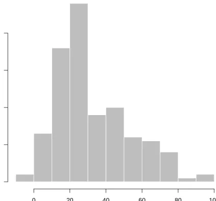
The output gives some information about how the algorithm ran. Each of the imputed datasets is now in the list a.out$imputations. Thus, we could plot a histogram of the tariff variable from the 3rd imputation,

> hist(a.out$imputations[[3]]$tariff, col="grey", border="white")

4.2.1 Saving imputed datasets

If you need to save your imputed datasets, one direct method is to save the output list from amelia,

> save(a.out, file = "imputations.RData")

As in the previous example, the ith imputed datasets can be retrieved from this list as a.out$imputations[[i]].

In addition, you can save each of the imputed datasets to its own file using the

(12)

Histogram of a.out$imputations[[3]]$tariff a.out$imputations[[3]]$tariff Frequency 0 20 40 60 80 100 0 10 20 30 40

(13)

> write.amelia(obj=a.out, file.stem = "outdata")

This will create one comma-separated value file for each imputed dataset in the following manner: outdata1.csv outdata2.csv outdata3.csv outdata4.csv outdata5.csv

Thewrite.ameliafunction can also save files in tab-delimited and Stata (.dta) file formats. For instance, to save Stata files, simply change the format argument to

"dta",

> write.amelia(obj=a.out, file.stem = "outdata", format = "dta")

Additionally,write.ameliacan create a “stacked” version of the imputed dataset which stacks each imputed dataset on top of one another. This can be done by setting the separate argument to FALSE. The resulting matrix is of size (N ·m)×p if the original dataset is excluded (orig.data = FALSE) and of size (N ·(m+ 1))×p if it is included (orig.data = TRUE). The stacked dataset will include a variable (set with impvar) that indicates to which imputed dataset the observation belongs. See Section 4.10 for a description of how to use this stacked dataset with the mi

commands in Stata.

4.2.2 Combining Multiple _Amelia Runs

The EMB algorithm is what computer scientists callembarrassingly parallel, meaning that it is simple to separate each imputation into parallel processes. With_Amelia it is simple to run subsets of the imputations on different machines and then combine them after the imputation for use in analysis model. This allows for a huge increase in the speed of the algorithm.

Output lists from different_Amelia runs can be combined together into a new list. For instance, suppose that we wanted to add another ten imputed datasets to our earlier call to amelia. First, run the function to get these additional imputations,

> a.out.more <- amelia(freetrade, m = 10, ts = "year", cs = "country", p2s=0) > a.out.more

Return code: 1

Chain Lengths:

---Imputation 1: 12

(14)

Imputation 3: 13 Imputation 4: 14 Imputation 5: 17 Imputation 6: 15 Imputation 7: 15 Imputation 8: 15 Imputation 9: 15 Imputation 10: 19

then combine this output with our original output using the ameliabind function,

> a.out.more <- ameliabind(a.out, a.out.more) > a.out.more

Return code: 1

Message: Normal EM convergence

Chain Lengths: ---Imputation 1: 14 Imputation 2: 15 Imputation 3: 9 Imputation 4: 14 Imputation 5: 10 Imputation 6: 12 Imputation 7: 13 Imputation 8: 13 Imputation 9: 14 Imputation 10: 17 Imputation 11: 15 Imputation 12: 15 Imputation 13: 15 Imputation 14: 15 Imputation 15: 19

This function binds the two outputs into the same output so that you can pass the combined imputations easily to analysis models and diagnostics. Note that

a.out.more now has a total of 15 imputations.

A simple way to execute a parallel processing scheme with _Amelia would be to run amelia with m set to 1 onm different machines or processors, save each output using the save function, load them all on the same R session using load command and then combine them using ameliabind. In order to do this, however, make sure to name each of the outputs a different name so that they do not overwrite each other when loading into the same R session. Also, some parallel environments will dump all generated files into a common directory, where they may overwrite each other. If it is convenient in a parallel environment to run a large number of amelia

(15)

calls from a single piece of code, one useful way to avoid overwriting is to create the

file.stem with a random suffix. For example:

> b<-round(runif(1,min=1111,max=9999)) > random.name<-paste("am",b,sep="")

> amelia <- write.amelia(obj=a.out, file.stem = random.name)

4.2.3 Screen Output

Screen output can be adjusted with the “print to screen” argument, p2s. At a value of 0, no screen printing will occur. This may be useful in large jobs or simulations where a very large number of imputation models may be required. The default value of 1, lists each bootstrap, and displays the number of iterations required to reach convergence in that bootstrapped dataset. The value of 2 gives more thorough screen output, including, at each iteration, the number of parameters that have significantly changed since the last iteration. This may be useful when the EM chain length is very long, as it can provide an intuition for many parameters still need to converge in the EM chain, and a sense of the time remaining. However, it is worth noting that the last several parameters can often take a significant fraction of the total number of iterations to converge. Setting p2s to 2 will also generate information on how EM algorithm is behaving, such as a ! when the current estimated complete data covariance matrix is not invertible and a*when the likelihood has not monotonically increased in that step. Having many of these two symbols in the screen output is an indication of a problematic imputation model7.

An example of the output when p2s is 2 would be

> amelia(freetrade, m = 1, ts = "year", cs = "country", p2s = 2)

amelia starting

beginning prep functions

Variables used: tariff polity pop gdp.pc intresmi signed fiveop usheg

running bootstrap Imputation 1

--setting up EM chain indicies

1(44) 2(34) 3(31) 4(25) 5(24) 6(23) 7(20) 8(17) 9(15) 10(14) 11(6) 12(6) 13(4) 14(2) 15(0)

saving and cleaning

Return code: 1

7_{Problems of non-invertible matrices often mean that current guess for the covariance matrix is}

singular. This is a sign that there may be two highly correlated variables in the model. One way to resolve is to use a ridge prior (see 4.7.1)

(16)

Chain Lengths:

---Imputation 1: 15

4.3 Parallel Imputation Using Multicore CPUs

Each imputation in the above EMB algorithm is completely independent of any other imputation, a property called embarrassingly parallel. This type of approach can take advantage of the multiple -core infrastructure of modern CPUs. Each core in a multi-core processor can execute independent operations in parallel. _Amelia can utilize this parallel processing internally via the parallel and the ncpus ar-guments. The parallelargument sets the parallel processing backend, either with

"multicore" or "snow" (or "no" for no parallel processing). The "multicore"

backend is not available on Windows systems, but tends to be quicker at parallel processing. On a Windows system, the "snow"backend provides parallel processing through a cluster of worker processes across the CPUs. You can set the default for this argument using the"amelia.parallel"option. This allows you to run Amelia in parallel as the default for an entire R session without setting arguments in the

amelia call.

For each of the parallel backends, _Amelia requires a number of CPUs to use in parallel. This can be set using thencpusargument. It can be higher than the number of physical cores in the system if hyperthreading or other technologies are available. You can use the parallel::detectCores function to determine how many cores are available on your machine. The default for this argument can be set using the

"amelia.ncpus" option.

On Unix-alike systems (such as Mac OS X and Linux distributions), the"multicore"

backend automatically sets up and stops the parallel workers by forking the process. On Windows, the "snow" backend requires more attention. _Amelia will attempt to create a parallel cluster of worker processes (since Windows systems cannot fork a process) and will stop this cluster after the imputations are complete. Alternatively,

Amelia also has a cl argument, which accepts a predefined cluster made using the parallel::makePSOCKcluster. For more information about parallel processing in R, see the documentation for the parallel package that ships along with R.

4.4 Imputation-improving Transformations

Social science data commonly includes variables that fail to fit to a multivariate normal distribution. Indeed, numerous models have been introduced specifically to deal with the problems they present. As it turns out, much evidence in the literature (discussed in King et al. 2001) indicates that the multivariate normal model used in _Amelia usually works well for the imputation stage even when discrete or non-normal variables are included and when the analysis stage involves these limited dependent variable models. Nevertheless, _Amelia includes some limited capacity to deal directly with ordinal and nominal variables and to modify variables that require other transformations. In general nominal and log transform variables should be declared to _Amelia, whereas ordinal (including dichotomous) variables often need

(17)

not be, as described below. (For harder cases, see (Schafer, 1997), for specialized MCMC-based imputation models for discrete variables.)

Although these transformations are taken internally on these variables to better fit the data to the multivariate normal assumptions of the imputation model, all the imputations that are created will be returned in the original untransformed form of the data. If the user has already performed transformations on their data (such as by taking a log or square root prior to feeding the data toamelia) these do not need to be declared, as that would result in the transformation occurring doubly in the imputation model. The fully imputed data sets that are returned will always be in the form of the original data that is passed to the amelia routine.

4.4.1 Ordinal

In much statistical research, researchers treat independent ordinal (including di-chotomous) variables as if they were really continuous. If the analysis model to be employed is of this type, then nothing extra is required of the of the imputation model. Users are advised to allow _Amelia to impute non-integer values for any missing data, and to use these non-integer values in their analysis. Sometimes this makes sense, and sometimes this defies intuition. One particular imputation of 2.35 for a missing value on a seven point scale carries the intuition that the respondent is between a 2 and a 3 and most probably would have responded 2 had the data been observed. This is easier to accept than an imputation of 0.79 for a dichotomous variable where a zero represents a male and a one represents a female respondent. However, in both cases the non-integer imputations carry more information about the underlying distribution than would be carried if we were to force the imputa-tions to be integers. Thus whenever the analysis model permits, missing ordinal observations should be allowed to take on continuously valued imputations.

In the freetrade data, one such ordinal variable is polity which ranges from -10 (full autocracy) to 10 (full democracy). If we tabulate this variable from one of the imputed datasets,

> table(a.out$imputations[[3]]$polity) -8 -7 -6 1 22 4 -5.80706995403517 -5 -4 1 7 3 -2 -1 2 9 1 7 3 4 5 7 15 26 5.73196387493741 6 7 1 13 5 8 9 36 13

(18)

we can see that there is one imputation between -4 and -3 and one imputation between 6 and 7. Again, the interpretation of these values is rather straightforward even if they are not strictly in the coding of the original Polity data.

Often, however, analysis models require some variables to be strictly ordinal, as for example, when the dependent variable will be modeled in a logistical or Pois-son regression. Imputations for variables set as ordinal are created by taking the continuously valued imputation and using an appropriately scaled version of this as the probability of success in a binomial distribution. The draw from this binomial distribution is then translated back into one of the ordinal categories.

For our data we can simply add polity to the ordsargument:

> a.out1 <- amelia(freetrade, m = 5, ts = "year", cs = "country", ords = + "polity", p2s = 0)

> table(a.out1$imputations[[3]]$polity)

-8 -7 -6 -5 -4 -2 -1 1 2 3 4 5 6 7 8 9

1 22 4 7 3 9 1 1 7 7 15 27 13 5 36 13

Now, we can see that all of the imputations fall into one of the original polity categories.

4.4.2 Nominal

Nominal variables8 _{must be treated quite differently than ordinal variables. Any}

multinomial variables in the data set (such as religion coded 1 for Catholic, 2 for Jewish, and 3 for Protestant) must be specified to_Amelia. In ourfreetradedataset, we havesigned which is 1 if a country signed an IMF agreement in that year and 0 if it did not. Of course, our first imputation did not limit the imputations to these two categories > table(a.out1$imputations[[3]]$signed) 0 0.223643650691989 0.332106092816539 142 1 1 0.416019978704527 1 1 26

In order to fix this for a p-category multinomial variable,_Amelia will determine p

(as long as your data contain at least one value in each category), and substitutep−1 binary variables to specify each possible category. These newp−1 variables will be treated as the other variables in the multivariate normal imputation method chosen, and receive continuous imputations. These continuously valued imputations will then be appropriately scaled into probabilities for each of the p possible categories, and one of these categories will be drawn, where upon the originalp-category multi-nomial variable will be reconstructed and returned to the user. Thus all imputations will be appropriately multinomial.

For our data we can simply add signed to the nomsargument:

8_{Dichotomous (two category) variables are a special case of nominal variables. For these}

(19)

Histogram of freetrade$tariff freetrade$tariff Frequency 0 20 40 60 80 100 0 5 10 15 20 25 30 35 Histogram of log(freetrade$tariff) log(freetrade$tariff) Frequency 1.5 2.0 2.5 3.0 3.5 4.0 4.5 5.0 0 10 20 30 40

Figure 3: Histogram of tariff and log(tariff).

> a.out2 <- amelia(freetrade, m = 5, ts = "year", cs = "country", noms = + "signed", p2s = 0)

> table(a.out2$imputations[[3]]$signed)

0 1

144 27

Note that _Amelia can only fit imputations into categories that exist in the original data. Thus, if there was a third category of signed, say 2, that corresponded to a different kind of IMF agreement, but it never occurred in the original data, _Amelia could not match imputations to it.

Since_Amelia properly treats ap-category multinomial variable asp−1 variables, one should understand the number of parameters that are quickly accumulating if many multinomial variables are being used. If the square of the number of real and constructed variables is large relative to the number of observations, it is useful to use a ridge prior as in section 4.7.1.

4.4.3 Natural Log

If one of your variables is heavily skewed or has outliers that may alter the imputation in an unwanted way, you can use a natural logarithm transformation of that variable in order to normalize its distribution. This transformed distribution helps _Amelia to avoid imputing values that depend too heavily on outlying data points. Log transformations are common in expenditure and economic variables where we have strong beliefs that the marginal relationship between two variables decreases as we move across the range.

For instance, figure 3 show the tariff variable clearly has positive (or, right) skew while its natural log transformation has a roughly normal distribution.

(20)

4.4.4 Square Root

Event count data is often heavily skewed and has nonlinear relationships with other variables. One common transformation to tailor the linear model to count data is to take the square roots of the counts. This is a transformation that can be set as an option in _Amelia.

4.4.5 Logistic

Proportional data is sharply bounded between 0 and 1. A logistic transformation is one possible option in _Amelia to make the distribution symmetric and relatively unbounded.

4.5 Identification Variables

Datasets often contain identification variables, such as country names, respondent numbers, or other identification numbers, codes or abbreviations. Sometimes these are text and sometimes these are numeric. Often it is not appropriate to include these variables in the imputation model, but it is useful to have them remain in the imputed datasets (However, there are models that would include the ID variables in the imputation model, such as fixed effects model for data with repeated observations of the same countries). Identification variables which are not to be included in the imputation model can be identified with the argument idvars. These variables will not be used in the imputation model, but will be kept in the imputed datasets.

If the year and country contained no information except labels, we could omit them from the imputation:

> amelia(freetrade, idvars = c("year", "country"))

Note that Amelia will return with an error if your dataset contains a factor or character variable that is not marked as a nominal or identification variable. Thus, if we were to omit the factor countryfrom the cs oridvars arguments, we would receive an error:

> a.out2 <- amelia(freetrade, idvars = c("year"))

Amelia Error Code: 38

The following variable(s) are characters: country

You may have wanted to set this as a ID variable to remove it from the imputation model or as an ordinal or nominal

variable to be imputed. Please set it as either and

try again.

In order to conserve memory, it is wise to remove unnecessary variables from a data set before loading it into _Amelia. The only variables you should include in your data when running _Amelia are variables you will use in the analysis stage and those variables that will help in the imputation model. While it may be tempting to simply mark unneeded variables as IDs, it only serves to waste memory and slow down the imputation procedure.

(21)

4.6 Time Series, or Time Series Cross Sectional Data

Many variables that are recorded over time within a cross-sectional unit are observed to vary smoothly over time. In such cases, knowing the observed values of obser-vations close in time to any missing value may enormously aid the imputation of that value. However, the exact pattern may vary over time within any cross-section. There may be periods of growth, stability, or decline; in each of which the observed values would be used in a different fashion to impute missing values. Also, these patterns may vary enormously across different cross-sections, or may exist in some and not others. _Amelia can build a general model of patterns within variables across time by creating a sequence of polynomials of the time index. If, for example, tariffs vary smoothly over time, then we make the modeling assumption that there exists some polynomial that describes the economy in cross-sectional unit i at timet as:

tariffti =β0+β1t+β1t2+β1t3. . . (9)

And thus if we include enough higher order terms of time then the pattern between observed values of the tariff rate can be estimated. _Amelia will create polynomials of time up to the user definedk-th order, (k≤3).

We can implement this with thets andpolytimearguments. If we thought that a second-order polynomial would help predict we could run

> a.out2 <- amelia(freetrade, ts = "year", cs = "country", polytime = 2)

With this input, _Amelia will add covariates to the model that correspond to time and its polynomials. These covariates will help better predict the missing values.

If cross-sectional units are specified these polynomials can be interacted with the cross-section unit to allow the patterns over time to vary between cross-sectional units. Unless you strongly believe all units have the same patterns over time in all variables (including the same constant term), this is a reasonable setting. When k

is set to 0, this interaction simply results in a model offixed effects where every unit has a uniquely estimated constant term. _Amelia does not smooth the observed data, and only uses this functional form, or one you choose, with all the other variables in the analysis and the uncertainty of the prediction, to impute the missing values. In order to impute with trends specific to each cross-sectional unit, we can set

intercsto TRUE:

> a.out.time <- amelia(freetrade, ts = "year", cs = "country", polytime = 2, + intercs = TRUE, p2s = 2)

Note that attempting to use polytime without the ts argument, or intercs

without thecs argument will result in an error.

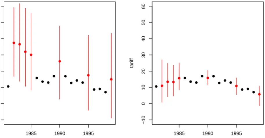
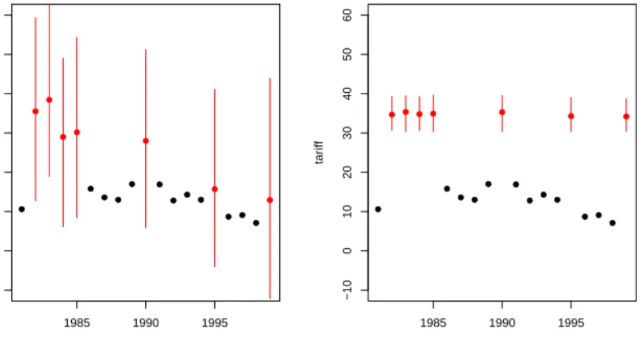
Using the tscsPlot function (discussed below), we can see in figure 4 that we have a much better prediction about the missing values when incorporating time than when we omit it:

> tscsPlot(a.out, cs = "Malaysia", main = "Malaysia (no time settings)", + var = "tariff", ylim = c(-10, 60))

> tscsPlot(a.out.time, cs = "Malaysia", main = "Malaysia (with time settings)", + var = "tariff", ylim = c(-10, 60))

(22)

● ● _● ● ● ● ● ● ● ● ● ● ● ● ● ● ● ● ● 1985 1990 1995 −10 0 10 20 30 40 50 60

Malaysia (no time settings)

time tar iff ● ● ● ● ● ● ● ● ● _● ● ● ● ● ● ● ● ● _● 1985 1990 1995 −10 0 10 20 30 40 50 60

Malaysia (with time settings)

time

tar

iff

Figure 4: The increase in predictive power when using polynomials of time. The panels shows mean imputations with 95% bands (in red) and observed data point (in black). The left panel shows an imputation without using time and the right panel includes polynomials of time.

4.6.1 Lags and Leads

An alternative way of handling time-series information is to include lags and leads of certain variables into the imputation model. Lags are variables that take the value of another variable in the previous time period whileleads take the value of another variable in the next time period. Many analysis models use lagged variables to deal with issues of endogeneity, thus using leads may seems strange. It is important to remember, however, that imputation models are predictive, not causal. Thus, since both past and future values of a variable are likely correlated with the present value, both lags and leads should improve the model.

If we wanted to include lags and leads of tariffs, for instance, we would simply pass this to the lags and leads arguments:

> a.out2 <- amelia(freetrade, ts = "year", cs = "country", lags = "tariff", + leads = "tariff")

4.7 Including Prior Information

Amelia has a number of methods of setting priors within the imputation model.

Two of these are commonly used and discussed below, ridge priors and observational priors.

4.7.1 Ridge Priors for High Missingness, Small n’s, or Large Correla-tions

When the data to be analyzed contain a high degree of missingness or very strong correlations among the variables, or when the number of observations is only slightly

(23)

greater than the number of parameters p(p+ 3)/2 (where p is the number of vari-ables), results from your analysis model will be more dependent on the choice of imputation model. This suggests more testing in these cases of alternative specifica-tions under_Amelia. This can happen when using the polynomials of time interacted with the cross section are included in the imputation model. In our running example, we used a polynomial of degree 2 and there are 9 countries. This adds 3×9−1 = 17 more variables to the imputation model (One of the constant “fixed effects” will be dropped so the model will be identified). When these are added, the EM algorithm can become unstable, as indicated by the vastly differing chain lengths for each imputation:

> a.out.time

Return code: 1

In these circumstances, we recommend adding a ridge prior which will help with numerical stability by shrinking the covariances among the variables toward zero without changing the means or variances. This can be done by including theempri

argument. Including this prior as a positive number is roughly equivalent to adding

empri artificial observations to the data set with the same means and variances as the existing data but with zero covariances. Thus, increasing the empri setting results in more shrinkage of the covariances, thus putting more a priori structure on the estimation problem: like many Bayesian methods, it reduces variance in return for an increase in bias that one hopes does not overwhelm the advantages in efficiency. In general, we suggest keeping the value on this prior relatively small and increase it only when necessary. A recommendation of 0.5 to 1 percent of the number of observations, n, is a reasonable starting value, and often useful in large datasets to add some numerical stability. For example, in a dataset of two thousand observations, this would translate to a prior value of 10 or 20 respectively. A prior of up to 5 percent is moderate in most applications and 10 percent is reasonable upper bound.

For our data, it is easy to code up a 1 percent ridge prior:

> a.out.time2 <- amelia(freetrade, ts = "year", cs = "country", polytime = 2, + intercs = TRUE, p2s = 0, empri = .01*nrow(freetrade)) > a.out.time2

(24)

●● ● ● ● ● ● ● ● ●● ● ● ● ● ● ● ● _● 1985 1990 1995 −10 0 10 20 30 40 50 60

Malaysia (no ridge prior)

time tar iff ● ● ● ● ● ● ● ● ● ● ● ● ● ● ● ● ● ● ● 1985 1990 1995 −10 0 10 20 30 40 50 60

Malaysia (with ridge prior)

time

tar

iff

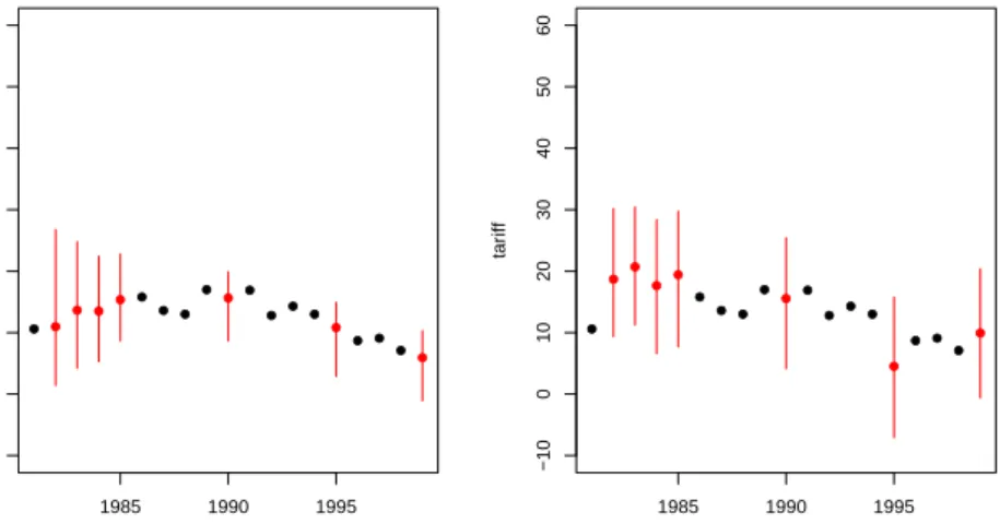
Figure 5: The difference in imputations when using no ridge prior (left) and when using a ridge prior set to 1% of the data (right).

Return code: 1

This new imputation model is much more stable and, as shown by using tscsPlot, produces about the same imputations as the original model (see figure 5):

> tscsPlot(a.out.time, cs = "Malaysia", main = "Malaysia (no ridge prior)", + var = "tariff", ylim = c(-10, 60))

> tscsPlot(a.out.time2, cs = "Malaysia", main = "Malaysia (with ridge prior)", + var = "tariff", ylim = c(-10, 60))

4.7.2 Observation-level priors

Researchers often have additional prior information about missing data values based on previous research, academic consensus, or personal experience. _Amelia can in-corporate this information to produce vastly improved imputations. The _Amelia algorithm allows users to include informative Bayesian priors about individual miss-ing data cells instead of the more general model parameters, many of which have little direct meaning.

(25)

The incorporation of priors follows basic Bayesian analysis where the imputation turns out to be a weighted average of the model-based imputation and the prior mean, where the weights are functions of the relative strength of the data and prior: when the model predicts very well, the imputation will down-weight the prior, and vice versa (Honaker and King, 2010).

The priors about individual observations should describe the analyst’s belief about the distribution of the missing data cell. This can either take the form of a mean and a standard deviation or a confidence interval. For instance, we might know that 1986 tariff rates in Thailand around 40%, but we have some uncertainty as to the exact value. Our prior belief about the distribution of the missing data cell, then, centers on 40 with a standard deviation that reflects the amount of uncertainty we have about our prior belief.

To input priors you must build a priors matrix with either four or five columns. Each row of the matrix represents a prior on either one observation or one variable. In any row, the entry in the first column is the row of the observation and the entry is the second column is the column of the observation. In the four column priors matrix the third and fourth columns are the mean and standard deviation of the prior distribution of the missing value.

For instance, suppose that we had some expert prior information about tariff rates in Thailand. We know from the data that Thailand is missing tariff rates in many years,

> freetrade[freetrade$country == "Thailand", c("year","country","tariff")]

year country tariff

153 1981 Thailand 32.3 154 1982 Thailand NA 155 1983 Thailand NA 156 1984 Thailand NA 157 1985 Thailand 41.2 158 1986 Thailand NA 159 1987 Thailand NA 160 1988 Thailand NA 161 1989 Thailand 40.8 162 1990 Thailand 39.8 163 1991 Thailand 37.8 164 1992 Thailand NA 165 1993 Thailand 45.6 166 1994 Thailand 23.3 167 1995 Thailand 23.1 168 1996 Thailand NA 169 1997 Thailand NA 170 1998 Thailand 20.1 171 1999 Thailand 17.1

Suppose that we had expert information that tariff rates were roughly 40% in Thailand between 1986 and 1988 with about a 6% margin of error. This corresponds

(26)

to a standard deviation of about 3. In order to include this information, we must form the priors matrix:

> pr <- matrix(c(158,159,160,3,3,3,40,40,40,3,3,3), nrow=3, ncol=4) > pr

[,1] [,2] [,3] [,4]

[1,] 158 3 40 3

[2,] 159 3 40 3

[3,] 160 3 40 3

The first column of this matrix corresponds to the row numbers of Thailand in these three years, the second column refers to the column number of tariff in the data and the last two columns refer to the actual prior. Once we have this matrix, we can pass it to amelia,

> a.out.pr <- amelia(freetrade, ts = "year", cs = "country", priors = pr)

In the five column matrix, the last three columns describe a confidence range of the data. The columns are a lower bound, an upper bound, and a confidence level between 0 and 1, exclusive. Whichever format you choose, it must be consistent across the entire matrix. We could get roughly the same prior as above by utilizing this method. Our margin of error implies that we would want imputations between 34 and 46, so our matrix would be

> pr.2 <- matrix(c(158,159,160,3,3,3,34,34,34,46,46,46,.95,.95,.95), nrow=3, ncol=5) > pr.2

[,1] [,2] [,3] [,4] [,5]

[1,] 158 3 34 46 0.95

[2,] 159 3 34 46 0.95

[3,] 160 3 34 46 0.95

These priors indicate that we are 95% confident that these missing values are in the range 34 to 46.

If a prior has the value 0 in the first column, this prior will be applied to all missing values in this variable, except for explicitly set priors. Thus, we could set a prior for the entire tariff variable of 20, but still keep the above specific priors with the following code:

> pr.3 <- matrix(c(158,159,160,0,3,3,3,3,40,40,40,20,3,3,3,5), nrow=4, ncol=4) > pr.3 [,1] [,2] [,3] [,4] [1,] 158 3 40 3 [2,] 159 3 40 3 [3,] 160 3 40 3 [4,] 0 3 20 5

(27)

4.7.3 Logical bounds

In some cases, variables in the social sciences have known logical bounds. Pro-portions must be between 0 and 1 and duration data must be greater than 0, for instance. Many of these logical bounds can be handled by using the correct trans-formation for that type of variable (see 4.4 for more details on the transtrans-formations handled by _Amelia). In the occasional case that imputations must satisfy certain logical bounds not handled by these transformations, _Amelia can take draws from a truncated normal distribution in order to achieve imputations that satisfy the bounds. Note, however, that this procedure imposes extremely strong restrictions on the imputations and can lead to lower variances than the imputation model im-plies. The mean value across all the imputed values of a missing cell is the best guess from the imputation model of that missing value. The variance of the distri-bution across imputed datasets correctly reflects the uncertainty in that imputation. It is often the mean imputed value that should conform to the any known bounds, even if individual imputations are drawn beyond those bounds. The mean imputed value can be checked with the diagnostics presented in the next section. In general, building a more predictive imputation model will lead to better imputations than imposing bounds.

Amelia implements these bounds by rejection sampling. When drawing the

im-putations from their posterior, we repeatedly resample until we have a draw that satisfies all of the logical constraints. You can set an upper limit on the number of times to resample with the max.resamplearguments. Thus, if after max.resample

draws, the imputations are still outside the bounds, _Amelia will set the imputation at the edge of the bounds. Thus, if the bounds were 0 and 100 and all of the draws were negative,_Amelia would simply impute 0.

As an extreme example, suppose that we know, for certain that tariff rates had to fall between 30 and 40. This, obviously, is not true, but we can generate imputations from this model. In order to specify these bounds, we need to generate a matrix of bounds to pass to the bounds argument. This matrix will have 3 columns: the first is the column for the bounded variable, the second is the lower bound and the third is the upper bound. Thus, to implement our bound on tariff rates (the 3rd column of the dataset), we would create the matrix,

> bds <- matrix(c(3, 30, 40), nrow = 1, ncol = 3) > bds

[,1] [,2] [,3]

[1,] 3 30 40

which we can pass to the bounds argument,

> a.out.bds <- amelia(freetrade, ts = "year", cs = "country", bounds = bds,

+ max.resample = 1000)

Imputation 1

(28)

Imputation 2 --1 2 3 4 5 6 7 8 9 10 11 12 13 14 15 16 Imputation 3 --1 2 3 4 5 6 7 8 9 10 11 12 13 14 15 Imputation 4 --1 2 3 4 5 6 7 8 9 10 11 12 13 14 15 16 Imputation 5 --1 2 3 4 5 6 7 8 9 10 11 12 13 14

The difference in results between the bounded and unbounded model are not obvious from the output, but inspection of the imputed tariff rates for Malaysia in figure 6 shows that there has been a drastic restriction of the imputations to the desired range:

> tscsPlot(a.out, cs = "Malaysia", main = "No logical bounds", var = + "tariff", ylim = c(-10,60))

> tscsPlot(a.out.bds, cs = "Malaysia", main = "Bounded between 30 and 40", var = + "tariff", ylim = c(-10,60))

Again, analysts should be extremely cautious when using these bounds as they can seriously affect the inferences from the imputation model, as shown in this example. Even when logical bounds exist, we recommend simply imputing variables normally, as the violation of the logical bounds represents part of the true uncertainty of imputation.

4.8 Diagnostics

Amelia currently provides a number of diagnostic tools to inspect the imputations

that are created.

4.8.1 Comparing Densities

One check on the plausibility of the imputation model is check the distribution of imputed values to the distribution of observed values. Obviously we cannot expect,

a priori, that these distribution will be identical as the missing values may differ

systematically from the observed value–this is fundamental reason to impute to begin with! Imputations with strange distributions or those that are far from the observed data may indicate that imputation model needs at least some investigation and possibly some improvement.

(29)

● ● ● ● ● ● ● ● ● ● ● ● ● ● ● ● ● ● ● 1985 1990 1995 −10 0 10 20 30 40 50 60 No logical bounds time tar iff ● ● ● ● ● ● ● ● ● ● ● ● ● ● ● ● ● ● ● 1985 1990 1995 −10 0 10 20 30 40 50 60

Bounded between 30 and 40

time

tar

iff

Figure 6: On the left are the original imputations without logical bounds and on the right are the imputation after imposing the bounds.

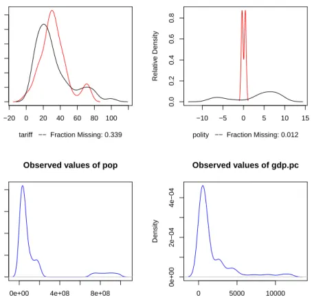
The plot method works on output from ameliaand, by default, shows for each variable a plot of the relative frequencies of the observed data with an overlay of the relative frequency of the imputed values.

> plot(a.out, which.vars = 3:6)

where the argument which.vars indicates which of the variables to plot (in this case, we are taking the 3rd through the 6th variables).

The imputed curve (in red) plots the density of themean imputation over them

datasets. That is, for each cell that is missing in the variable, the diagnostic will find the mean of that cell across each of themdatasets and use that value for the density plot. The black distributions are the those of the observed data. When variables are completely observed, their densities are plotted in blue. These graphs will allow you to inspect how the density of imputations compares to the density of observed data. Some discussion of these graphs can be found in Abayomi, Gelman and Levy (2008). Minimally, these graphs can be used to check that the mean imputation falls within known bounds, when such bounds exist in certain variables or settings.

We can also use the function compare.density directly to make these plots for an individual variable:

> compare.density(a.out, var = "signed") 4.8.2 Overimpute

Overimputing is a technique we have developed to judge the fit of the imputation

model. Because of the nature of the missing data mechanism, it is impossible to tell whether the mean prediction of the imputation model is close to the unobserved value that is trying to be recovered. By definition this missing data does not exist to

(30)

−20 0 20 40 60 80 100

0.000

0.010

0.020

0.030

Observed and Imputed values of tariff

tariff −− Fraction Missing: 0.339

Relativ e Density −10 −5 0 5 10 15 0.0 0.2 0.4 0.6 0.8

Observed and Imputed values of polity

polity −− Fraction Missing: 0.012

Relativ

e Density

0e+00 4e+08 8e+08

0e+00

4e−09

8e−09

Observed values of pop

N = 171 Bandwidth = 2.431e+07 Density 0 5000 10000 0e+00 2e−04 4e−04 Observed values of gdp.pc N = 171 Bandwidth = 490.6 Density

Figure 7: The output of the plot method as applied to output from amelia. In the upper panels, the distribution of mean imputations (in red) is overlayed on the distribution of observed values (in black) for each variable. In the lower panels, there are no missing values and the distribution of observed values is simply plotted (in blue). Note that now imputed tariff rates are very similar to observed tariff rates, but the imputation of the Polity score are quite different. This is plausible if different types of regimes tend to be missing at different rates.

(31)

create this comparison, and if it existed we would no longer need the imputations or care about their accuracy. However, a natural question the applied researcher will often ask is how accurate are these imputed values?

Overimputing involves sequentially treating each of the observed values as if they had actually been missing. For each observed value in turn we then generate several hundred imputed values of that observed value, as if it had been missing. While m= 5 imputations are sufficient for most analysis models, this large number of imputations allows us to construct a confidence interval of what the imputed value would have been, had any of the observed data been missing. We can then graphically inspect whether our observed data tends to fall within the region where it would have been imputed had it been missing.

For example, we can run the overimputation diagnostic on our data by running

> overimpute(a.out, var = "tariff")

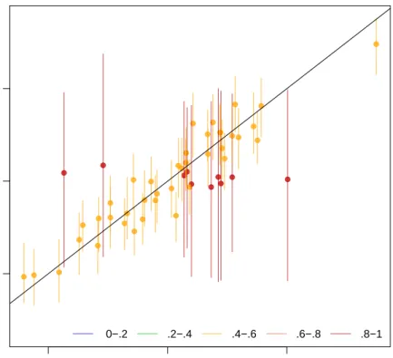
Our overimputation diagnostic, shown in Figure 8, runs this procedure through all of the observed values for a user selected variable. We can graph the estimates of each observation against the true values of the observation. On this graph, a y=x

line indicates the line of perfect agreement; that is, if the imputation model was a perfect predictor of the true value, all the imputations would fall on this line. For each observation, _Amelia also plots 90% confidence intervals that allows the user to visually inspect the behavior of the imputation model. By checking how many of the confidence intervals cover the y =x line, we can tell how often the imputation model can confidently predict the true value of the observation.

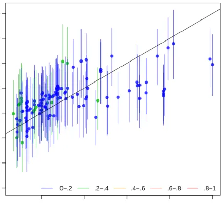
Occasionally, the overimputation can display unintuitive results. For example, different observations may have different numbers of observed covariates. If covari-ates that are useful to the prediction are themselves missing, then the confidence interval for this observation will be much larger. In the extreme, there may be ob-servations where the observed value we are trying to overimpute isthe only observed value in that observation, and thus there is nothing left to impute that observation with when we pretend that it is missing, other than the mean and variance of that variable. In these cases, we should correctly expect the confidence interval to be very large.

An example of this graph is shown in figure 9. In this simulated bivariate dataset, one variable is overimputed and the results displayed. The second variable is either observed, in which case the confidence intervals are very small and the imputa-tions (yellow) are very accurate, or the second variable is missing in which case this variable is being imputed simply from the mean and variance parameters, and the imputations (red) have a very large and encompassing spread. The circles represent the mean of all the imputations for that value. As the amount of missing information in a particular pattern of missingness increases, we expect the width of the confi-dence interval to increase. The color of the conficonfi-dence interval reflects the percent of covariates observed in that pattern of missingness, as reflected in the legend at the bottom.

(32)

20 40 60 80 100 −40 −20 0 20 40 60 80 100

Observed versus Imputed Values of tariff

Observed Values

Imputed V

alues

0−.2 .2−.4 .4−.6 .6−.8 .8−1

Figure 8: An example of the overimputation diagnostic graph. Here ninety percent confidence intervals are constructed that detail where an observed value would have been imputed had it been missing from the dataset, given the imputation model. The dots represent the mean imputation. Around ninety percent of these confidence intervals contain the y = x line, which means that the true observed value falls within this range. The color of the line (as coded in the legend) represents the fraction of missing observations in the pattern of missingness for that observation.

(33)

0.0 0.5 1.0

0.0

0.5

1.0

Observed versus Imputed Values

Observed Values

Imputed V

alues

0−.2 .2−.4 .4−.6 .6−.8 .8−1

Figure 9: Another example of the overimpute diagnostic graph. Note that the red lines are those observations that have fewer covariates observed and have a higher variance across the imputed values.

(34)

4.8.3 Overdispersed Starting Values

If the data given to _Amelia has a poorly behaved likelihood, the EM algorithm can have problems finding a global maximum of the likelihood surface and starting values can begin to effect imputations. Because the EM algorithm is deterministic, the point in the parameter space where you start it can impact where it ends, though this is irrelevant when the likelihood has only one mode. However, if the starting values of an EM chain are close to a local maximum, the algorithm may find this maximum, unaware that there is a global maximum farther away. To make sure that our imputations do not depend on our starting values, a good test is to run the EM algorithm from multiple, dispersed starting values and check their convergence. In a well behaved likelihood, we will see all of these chains converging to the same value, and reasonably conclude that this is the likely global maximum. On the other hand, we might see our EM chain converging to multiple locations. The algorithm may also wander around portions of the parameter space that are not fully identified, such as a ridge of equal likelihood, as would happen for example, if the same variable were accidentally included in the imputation model twice.

Amelia includes a diagnostic to run the EM chain from multiple starting values

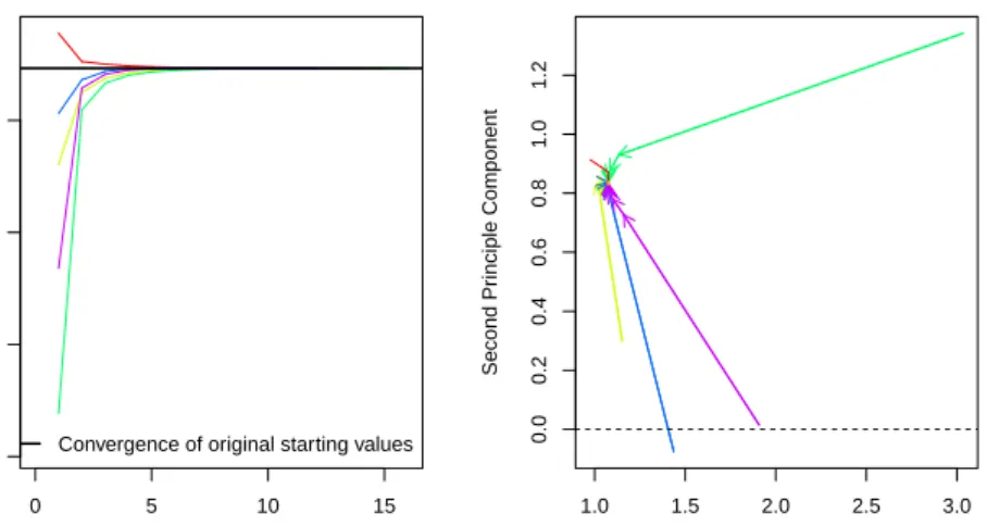
that are overdispersed from the estimated maximum. The overdispersion diagnostic will display a graph of the paths of each chain. Since these chains move through spaces that are in an extremely high number of dimensions and can not be graphically displayed, the diagnostic reduces the dimensionality of the EM paths by showing the paths relative to the largest principle components of the final mode(s) that are reached. Users can choose between graphing the movement over the two largest principal components, or more simply the largest dimension with time (iteration number) on the x-axis. The number of EM chains can also be adjusted. Once the diagnostic draws the graph, the user can visually inspect the results to check that all chains convergence to the same point.

For our original model, this is a simple call to disperse:

> disperse(a.out, dims = 1, m = 5) > disperse(a.out, dims = 2, m = 5)

where m designates the number of places to start EM chains from and dims are the number of dimensions of the principal components to show.

In one dimension, the diagnostic plots movement of the chain on the y-axis and time, in the form of the iteration number, on the x-axis. Figures 10 show two examples of these plots. The first shows a well behaved likelihood, as the starting values all converge to the same point. The black horizontal line is the point where

Amelia converges when it uses the default method for choosing the starting values.

The diagnostic takes the end point of this chain as the possible maximum and disperses the starting values away from it to see if the chain will ever finish at another mode.

4.8.4 Time-series plots

As discussed above, information about time trends and fixed effects can help produce better imputations. One way to check the plausibility of our imputation model is

(35)

0 5 10 15

−0.5

0.0

0.5

1.0

Overdispersed Start Values

Number of Iterations

Largest Pr

inciple Component

Convergence of original starting values

1.0 1.5 2.0 2.5 3.0 0.0 0.2 0.4 0.6 0.8 1.0 1.2

Overdispersed Starting Values

First Principle Component

Second Pr

inciple Component

Figure 10: A plot from the overdispersion diagnostic where all EM chains are con-verging to the same mode, regardless of starting value. On the left, the y-axis represents movement in the (very high dimensional) parameter space, and the x -axis represents the iteration number of the chain. On the right, we visualize the parameter space in two dimensions using the first two principal components of the end points of the EM chains. The iteration number is no longer represented on the

y-axis, although the distance between iterations is marked by the distance between arrowheads on each chain.

to see how it predicts missing values in a time series. If the imputations for the Malaysian tariff rate were drastically higher in 1990 than the observed years of 1989 or 1991, we might worry that there is a problem in our imputation model. Checking these time series is easy to do with the tscsPlot command. Simply choose the variable (with the var argument) and the cross-section (with the cs argument) to plot the observed time-series along with distributions of the imputed values for each missing time period. For instance, we can run

> tscsPlot(a.out.time, cs = "Malaysia", main = "Malaysia (with time settings)", + var = "tariff", ylim = c(-10, 60))

to get the plot in figure 11. Here, the black point are observed tariff rates for Malaysia from 1980 to 2000. The red points are the mean imputation for each of the missing values, along with their 95% confidence bands. We draw these bands by imputing each of missing values 100 times to get the imputation distribution for that observation.

(36)

● ● ● ● ● ● ● _● ● ● ● ● ● ● ● ● ● ● ● 1985 1990 1995 −10 0 10 20 30 40 50 60

Malaysia (with time settings)

time

tar

iff

Figure 11: Tariff rates in Malaysia, 1980-2000. An example of thetscsPlotfunction, the black points are observed values of the time series and the red points are the mean of the imputation distributions. The red lines represent the 95% confidence bands of the imputation distribution.

AMELIA II: A Program for Missing Data

AMELIA II

: A Program for Missing Data

James Honaker, Gary King, and Matthew Blackwell

Version 1.7.4

December 5, 2015

Contents

1

Introduction

2

What

A

melia Does

2.1

Assumptions

2.2

Algorithm

2.3

Analysis

3

Versions of

A

melia

3.1

Installation and Updates from R

3.2

Installation in Windows of

A

melia

V

iew as a Standalone

Program

3.3

Linux (local installation)

4

A User’s Guide

4.1

Data and Initial Results

4.2

Multiple Imputation

4.3

Parallel Imputation Using Multicore CPUs

4.4

Imputation-improving Transformations

4.5

Identification Variables

4.6

Time Series, or Time Series Cross Sectional Data

4.7

Including Prior Information

4.8

Diagnostics

_A

_A

_A

_V