ABSTRACT
BHATTACHARYYA, ABHISHA. Evaluating Generalized Path Queries by Integrating Algebraic Path Problem Solving with Graph Pattern Matching. (Under the direction of Dr. Kemafor Anyanwu Ogan.) Path querying on Semantic Networks is gaining increased focus because of its broad applicability. Some graph databases offer support for variants of path queries e.g. shortest path. However, many applications have the need for the set version of various path problem i.e. finding paths between multiple source and multiple destination nodes (subject to different kinds of constraints). Further, the sets of source and destination nodes may be described declaratively as patterns, rather than given explicitly. Such queries lead to the requirement of integrating graph pattern matching with path problem solving. There are currently existing limitations in support of such queries (either inability to express some classes, incomplete results, inability to complete query evaluation unless graph patterns are extremely selective, etc).
Evaluating Generalized Path Queries by Integrating Algebraic Path Problem Solving with Graph Pattern Matching
by
Abhisha Bhattacharyya
A thesis submitted to the Graduate Faculty of North Carolina State University
in partial fulfillment of the requirements for the Degree of
Master of Science
Computer Science
Raleigh, North Carolina 2019
APPROVED BY:
Dr. Rada Chirkova Dr. Nagiza Samatova
DEDICATION
BIOGRAPHY
ACKNOWLEDGEMENTS
I am indebted to my advisor, my committee members, my peers and my family without whom I would never have finished my thesis. First and foremost, I would like to express my sincerest gratitude to my advisor, Dr. Kemafor Anyanwu Ogan who gave me the opportunity to join her lab even before I was a student and then gave me a recommendation letter which helped me immensely in getting accepted in the graduate program at NC State. Without her continuous help, support and guidance I would not have gotten my masters degree. I also thank Dr. Rada Chirkova and Dr. Nagiza Samatova for serving on my thesis committee.
I would like to acknowledge the support of my past and present lab members, HyeongSik Kim, Ruth Okoilu, Shalki Shrivastava, Sidan Gao, Akanksha Mohan and Arunkumar Krishnamoorthy. I would like to specially thank HyeongSik Kim for taking time to help me out and giving me valuable knowledge which helped me immensely in my research work.
Last but not the least, I would like to extend my deepest gratitude to my family, particularly, my parents, Sujit Bhattacharyya and Kaberi Bhattacharyya and my brother, Arkajyoti Bhattacharyya for their constant support and words of encouragement which helped me tide over the difficult perids of my life and career. I would also, like to wholeheartedly thank my husband, Punnag Chatterjee, for encouraging me to get into graduate studies and supporting me immensely during the stressful periods of graduate school. Without my family I would not be where I am today.
TABLE OF CONTENTS
LIST OF FIGURES. . . vii
Chapter 1 INTRODUCTION . . . 1
1.1 Motivation . . . 3
1.2 Observation . . . 5
1.3 Structure of the Thesis . . . 6
Chapter 2 RELATED WORK. . . 7
2.1 Graph Theoretic Approach . . . 7
2.2 Algebraic Approach . . . 8
2.2.1 Relational Algebra (Database Approach) . . . 8
2.2.2 Hybrid Approach (Partially Relational+Graph Approach) . . . 8
2.2.3 Total Algebraic Approach (Relational Algebra*+Path Algebra) . . . 10
Chapter 3 BACKGROUND. . . 12
3.1 Algebraic Path Problem Solving . . . 12
3.2 RDF . . . 15
3.2.1 RDF Data Model . . . 15
3.3 Algebraic Query Evaluation of Graph Pattern Matching . . . 17
3.3.1 Apache Jena . . . 18
3.4 Semstorm . . . 19
3.4.1 Apache Tez . . . 20
3.4.2 Loops and Cycles: . . . 20
3.5 Serpent . . . 20
Chapter 4 APPROACH . . . 21
4.1 Query Expression . . . 22
4.1.1 Identifying GPQ Sub-Query Components in SPARQL* Queries: . . . 23
4.1.2 Implementation Strategy: . . . 23
4.2 Query Compilation . . . 25
4.2.1 Logical Query Plan Transformation: . . . 26
4.3 Query Execution . . . 27
4.3.1 Implementation Strategy . . . 27
4.4 Path Constraints . . . 29
4.5 User Interface Updations: . . . 29
Chapter 5 EVALUATION . . . 31
5.1 Test setup . . . 31
5.1.1 Dataset and Queries: . . . 31
5.1.2 Hardware Configuration: . . . 32
5.2 Evaluation Results . . . 32
5.2.1 Performance Evaluation: . . . 32
5.2.3 Expressiveness: . . . 34
5.2.4 Query Compilation Time Comparison: . . . 36
5.3 List of Queries . . . 36
5.3.1 Small Queries . . . 37
5.3.2 Large Queries . . . 40
Chapter 6 CONCLUSION AND FUTURE WORK . . . 45
BIBLIOGRAPHY . . . 46
APPENDIX . . . 49
Appendix A CODE . . . 50
LIST OF FIGURES
Figure 1.1 QueryPlan . . . 5
Figure 2.1 Categories of Existing Platforms . . . 8
Figure 3.1 Example graph, Path Expression and Path Sequence . . . 13
Figure 3.2 Example explaining Path Sequence . . . 14
Figure 3.3 Example showing a few steps of the SOLVE algorithm for sources=1 . . . 15
Figure 3.4 RDF Data Model: Table showing example RDF triples . . . 16
Figure 3.5 RDF Data Model: Triples represented in the form of graph with directed edges 17 Figure 3.6 Example SPARQL query and its transformation after compilation by Jena’s parser (a) Example query (b) Corresponding SSE . . . 19
Figure 4.1 (a) An example path query in our implementation of the integrated platform (b) The SSE produced by Jena’s parser and compiler . . . 22
Figure 4.2 Mapping of the parts of motivating example to components of gpq . . . 25
Figure 4.3 Query plan transformation from graph pattern matching query to gpq . . . 26
Figure 4.4 The Tez DAG representating the physical plan for the query shown in Figure 4.1(a) . . . 28
Figure 5.1 Size of source and destination sets for each query . . . 32
Figure 5.2 Number of paths comparison . . . 33
Figure 5.3 Explanation of self-loops (a) Example graph (b) Comparison of the paths found by Sem-Ser vs Stardog . . . 34
Figure 5.4 Time taken per path (a) For Small Queries (b) For Large Queries . . . 34
Figure 5.5 Execution Time of constrained queries vs unconstrained queries . . . 35
Figure 5.6 Table showing comparison of the level of expressiveness of our platform with Neo4j and Stardog . . . 35
CHAPTER
1
INTRODUCTION
Many applications have the need to find connections between entities in data sets. In graph theoretic terms, this amounts to querying for paths in graphs, between sources and destinations. For most real world applications in such scenarios, the connection sought is not usually between a singe source and single destination but multiple source and destination nodes. Often the sets of sources and destinations cannot be easily given explicitly but these can rather be described declaratively in terms of patterns to be matched in graphs.
level)or otherstructural constraints. Such constraints are more expressive than the property path queries which requires a regular expression of the properties in path being searched for. In a sense, these queries are traditional path queries generalized to include graph patterns and path constraints. We refer to such queries asGeneralized Path Queries - gpqs.
With the standardization of property path expressions in SPARQL, there is increased focus on graph traversal queries. However, property path queries have a fundamental difference besides their expressiveness when compared to path queries - the result of a property path expression is not the paths connecting the source and destination nodes but rather sets of source and destination nodes connected by paths that match the property path pattern. G-Core[Ang18]presents a good discussion of classes of these queries. For graph-based query engines such as Neo4j[Neo], StarDog [Sta], Allegrogaph[Aas06], AnzoGraph[Anz], Virtuoso[EM09]that support the RDF model, there is varied support for path querying. Some other earlier platform such as[GA13a] [Gao18] [Gao10] [Fio12] [PZ11] [GN]has focused exclusively on the path querying
A common thread across existing path querying evaluation strategies is that they are built on traditional graph algorithms. The challenge with graph theoretic interpretations of such queries is that the different constraints in gpqs may translate to different classes of graph problems, requiring different algorithms. For example, shortest path algorithms vs. subgraph isomorphism algorithms vs. subgraph homeomorphism, and so on. From the point of view of query processing, this is a limited approach because of the limited opportunity for decomposition and reusability. On the other hand, adopting an algebraic perspective allows problems to be interpreted in a more generalized form. This also allows for more natural integration with algebraic graph pattern query engines. Considering such a strategy makes sense once one observes that gpqs are essentially comprised of four elements: graph pattern matching, joining/filtering of graph patterns, path computation, path filtering. There are only a few platforms that do allow the sources and destinations to be expressed in a more generalized manner (for example using a graph pattern to describe the source and destination nodes). But these usually employ a graph theoritical approach of computing the paths. Some existing platforms like[Sta]do partially interpret gpq-like queries algebraically. However, the absence of a complete algebraic query interpretation framework results on falling back on traditional graph algorithms in many situations.
In this thesis, such an algebraic approach has been proposed to evaluate Generalized Path Queries (gpqs). Since determining the exact sources and destinations for a particular path query involves simple graph pattern matching, graph computation is not required for it. We propose to use existing pattern matching approaches, for example Union of Conjunctive Queries to compute the exact sources and destinations and then add the path computation operator at the root of the query plan. This approach works because we possess the knowledge that path computation would always be the last step of query computation, i.e., the output of the graph pattern matching would feed into the path computation operator. This thesis also describes two different implementation models for the algebraic approach: the deep approach and the lightweight approach. An example integration using existing graph pattern matching platform and path computation platform has been shown. A comparative study has also been done between the integrated platform and other platforms that can handle such generalized path queries.
1.1
Motivation
There are a lot of applications that require path query computation for multiple sources and mul-tiple destinations and in most cases the sources and destinations will not be explicitly stated but described declaratively. One possible application of this type of path query isFlight and Airport Risk Assessment(which has been described in[Any07]). To determine potential threats to flight and airport safety, security officials would query for and investigate all high risk passengers scheduled for the flight. An example query could be find the relationships betweenpassengers scheduled for flights to Washington DC, who purchased their tickets by cash or purchased their tickets less than a day before departure, andhave links to flight training. Another example query in the same scenario would be finding connections withfinancial linksbetweenpassengers who fall within a certain demographic on a particular flightandknown groups that endorse extremism or countries that support such groups.
Another possible application isLocal Threat Assessment. To determine threats to local safety, for example, to prevent an attack like the San Bernardino Shooting incident[San], the local security officials would want to regularly query and investigate high risk residents in the locality. An example query for this purpose would be finding the relationships betweenresidents who recently purchased weapons or are frequent visitors at a shooting range, and have been in touch with any person suspected of terrorism. An important point to be noted for this example query is that the source and destination sets are the same and we are trying to find connections between the members of the set. Here, security officials may also be interested insocial media links that show if the person likes or follows posts from known extremist groups.
declaratively (for example,passengers scheduled for flights to Washington DC, who purchased their tickets by cashorgroups that endorse extremism). The resulting paths are also subject to some constraints (for example,associated with flight training orfinancial linksorsocial media links to extremist groups). Such queries can have very important applications where network analysis plays a significant role. Thus, an integrated system that can take declarative descriptions of the sources, destinations and required constraints (if any) and produce qualifying paths and connections between the sources and destinations would have a wide range of real-world applications.
There are several different ways to try to approach this problem, and the first one is a graph theoritical approach. The problems we are trying to solve are homeomorphic in nature for which graph traversal based algorithm can be developed, but such algorithms are NP hard. Also such graph traversal algorithms usually require the whole graph to be in memory to be able to produce correct and consistent results. Pure graph traversal algorithms also have a few other disadvantages. Firstly, such algorithms assume explicit definitions of the source and destination nodes. Such explicit definitions are not always available for a lot of practical problems as seen in the examples described earlier. Secondly, the problems we are dealing with are a class or set of problems where addition of a new constraint makes it a slightly different problem in the same set. Pure graph algorithms would have to approach each problem separately and have different solutions to each problem in the set. Thirdly, graph algorithms are notoriously difficult to parallelize, for example, depth-first-search algorithm is inherently sequential.
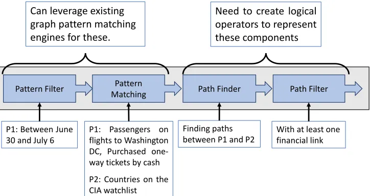
The alternative to pure graph algorithms is analgebraic interpretationof the problem where query evaluation can be represented by an expression that is composed of multiple operators in a defined order. In each of the scenarios described earlier four distinct components can be distinguished clearly.
1. Pattern matching, to interpret the sets of source and destination nodes which have been described declaratively.
2. Pattern filtering, to filter out unnecessary triples.
3. Path problem solving, to find the actual links between the set of sources and destinations. 4. Path constraint filtering, to filter out irrelevant paths according to the given conditions.
1.2
Observation
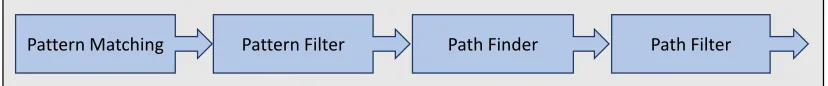
The first component which is the graph pattern matching can be solved using any existing pattern matching platforms. For the second and third components,[Tar79b] [Tar79a]discusses the basic idea behind an algebraic technique for solving path problems, where a variety of path problems can be interpreted in terms of sum and product operations. There is also some recent work on this in[Any07]which shows the overall architecture of such an integrated system and also the query evaluation plan. Figure 1.1 shows the implementation plan proposed in[Any07]. Here thePattern matching andPattern Filtersteps can be taken care of by any existing graph pattern matching platform. For thePath FinderandPath Filtersteps we would need a path operator for the algebraic approach.
Usually in such scenarios, where different queries on a dataset differ only slightly from each other, there is a lot of overlap between the answers to those queries, many of them tending to sharing sub-expressions and sub paths. The algebraic approach makes query evaluation much more amenable to multi-query optimization since this approach allows reuse of the common sub-expressions. The most commonly occurring sub-expressions and sub-paths may be computed only once and then reused for each subsequent query as necessary.
In this thesis, we propose an algebraic query evaluation technique for gpqs that delineates the four gpqs subquery elements and their mapping to algebraic query operations so that gpqs query planning translates to composition and ordering of query operations. More specifically, the thesis presents
• a conceptual query evaluation model that integrates algebraic graph pattern matching with algebraic path problem solving.
• an implementation model that perturbs the plan for graph pattern matching query generated by a SPARQL query compiler by splicing in algebraic path querying operators to produce a gpqs query plan. Another advantage of this strategy is that current SPARQL parsers and existing graph pattern matching compiler can be adopted without modification.
• an example implementation strategy using Apache Jena’s query compiler and Apache Tez’ DAG for physical execution is presented.
Path Filter Path Finder
Pattern Filter Pattern Matching
• comparison of the performance and expressiveness of the integrated platform with a popular engine.
1.3
Structure of the Thesis
The thesis has been subdivided into five chapters, where the first Chapter gives a brief introduction to the topic, motivation behind the research and the contributions of the thesis.
The background of the research has been discussed in the second Chapter. This chapter contains information about the RDF data model, SPARQL querying language, graph pattern matching, path querying etc. The second chapter also introduces the open source Apache Jena[McB02]framework for RDF storage and SPARQL query processing, the Apache Tez[Tez]project which is used to build application frameworks that allows for a complex directed-acyclic-graph of tasks for processing data. Apart from the tools and models, this chapter also includes an introduction to SemStorm[Kim17b] and the PrefixSolve algorithm[GA13b]. SemStorm is a query processing and storage framework for large-scale knowledge graph. The PrefixSolve algorithm is an implementation framework that allows efficient querying of graphs on disk. The code changes involved in the thesis topic has been built on the existing code base these two projects. More explanation regarding these two platforms can be found in the second Chapter of this thesis.
The third chapter includes the literature study required for the research like existing integrated platforms and their disadvantages. The fourth chapter discusses the approach used for the integra-tion of Semstorm’s processing followed by path query computaintegra-tion on the input dataset using a single query. This chapter also includes implementation details.
CHAPTER
2
RELATED WORK
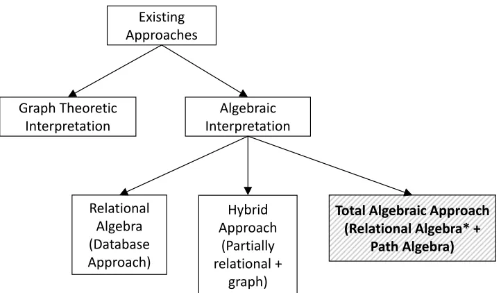
[AG08][Woo12]provides a good survey of graph query languages. Figure 2.1 shows the categories that existing platforms can be divided into. Existing approaches can be divided into two main cate-gories: Graph Theoretic Approach and Algebraic Approach. The Algebraic Approach can be further sub-divided into Relational Algebra (Database Approach), Hybrid Approach (Partially Relational+ Graph Approach) and Total Algebraic Approach (Relational Algebra*+Path Algebra). Each of these categories are explained in detail in the next few sections.
2.1
Graph Theoretic Approach
Existing Approaches
Graph Theoretic Interpretation
Algebraic Interpretation
Relational Algebra (Database Approach)
Hybrid Approach
(Partially relational +
graph)
Total Algebraic Approach (Relational Algebra* +
Path Algebra)
Figure 2.1Categories of Existing Platforms
2.2
Algebraic Approach
The second method of query evaluation is an algebraic approach where query operators act as the building blocks of query evaluation and are composed by an optimizer.
2.2.1 Relational Algebra (Database Approach)
In this approach introduced by[GN]the nodes on the paths are interpreted in terms of joins. The Database approach Hence, every edge with start and end nodes is joined with the next edge with start and end nodes thus forming paths. For queries using this approach the length of the resulting path must be bound since the query needs to specify the number of joins expected in the path. If the dataset is partitioned into different tables based on any parameter, the query would need to specify the tables that have to be joined. Since the number of tables mentioned in the query must be bound, this approach cannot find paths of arbitrary length. Also, the approach is mostly focused on efficiently finding shortest path.
2.2.2 Hybrid Approach (Partially Relational+Graph Approach)
provides a limited range of path constraints. Similar to the previous category these platforms also focus on shortest path queries, and cannot efficiently run all-paths queries.
Neo4j[Neo], AgensGraph[Age]uses Cypher[Fra18][Cyp]as its query language. Cypher uses a fast bidirectional breadth-first search algorithm for optimizing path queries. However, this algorithm can be used only in certain scenarios. Firstly, this algorithm can only be used for finding shortest path, when finding all paths Neo4j uses a much slower exhaustive depth-first search algorithm. Even when finding shortest paths the fast algorithm is used only if the predicates in the path query can be evaluated on the fly while searching for the path. In case of predicates that need to look at the full path before deciding whether to keep or discard that particular path Neo4j’s query evaluation must fall back to exhaustive searching.
Triples that have a constant as the object are considered as properties of the subject node. For example after loading the triple
acm:person-297809 akt:full -name "Wendy E. Mackay"
into Neo4j the node identified byacm:person-297809would have a propertyfull-namewith the value"Wendy E. Mackay". Now suppose we have a shortest path query with the predicate that saysALL nodes in the path must have a full-name property. This predicate can be evaluated on the fly while running the query and thus this query will be evaluated using the fast bidirectional breadth-first search algorithm. However, suppose the the predicate in the above query wasAt least one node in the path must have a full-name property. To evaluate this query Neo4j needs to inspect the whole path before it can decide whether the path meets the requirements. Thus, for this query exhaustive depth-first search algorithm will be used. Neo4j’s Cypher also has another drawback where it’s shortest path algorithm does not work when the start and end nodes are the same. Such a scenario might occur when performing a shortestPath search where the sources and destinations are overlapping sets of nodes. This error can be avoided by changing certain configuration parameters, but, in that case there might be some missing results. Also this issue does not occur when running all paths queries.Stardog follows a more traditional SPARQL operators for query evaluation. For any path query with start and end variable patterns Stardog uses the below evaluation strategy
eval(PQ(s, PS, e, PE, PQ) = Join(PS, Join(PE, eval(PQ(s, e, PQ), DG)))
resultset which will then need to be joined with the start and end patterns. Figure??shows some of the existing platforms and the algorithms used by these platforms.
There is another hybrid approach that is followed by platforms such as Virtuoso[EM09], RDFPath [PZ11], Blazegraph[Bla], Gremlin[Rod15]which is the query language for JanusGraph[Jan]and Nep-tune[Nep], Oracle’s PGQL[Res16][Sev16][Ora][Pgq]which use Path expression queries. Their focus is on patterns for path constructs and they do not have any provision for patterns for sources and desti-nations. These platforms require users to write a regular expression of the properties in the path and the result of the query is the set of sources and destinations and not necessarily the paths between them. To write a regular expression the users need to possess the knowledge of the properties in the path and also a general ordering of the properties.
?a akt:has-author/akt:has-affiliation*
?b.
is an example query which is looking for paths that has one "has-author" property and zero or more "has-affiliation" properties.Virtuoso, RDFPath and Blazegraph use property paths which is a route through a graph between two graph nodes. SPARQL 1.1[HS]supports these property paths[Pro]which allows the extension of matching triple patterns to arbitrary length paths. However, using property paths it is only possible to know the specific sources and destination, but not the exact paths. Gremlin also requires the predicates of the path to be specified in the query. Oracle’s PGQL finds paths using general expressions over vertices and edges of the graph. In this case, like in the case of property paths the user needs to have the knowledge of the sequence of edges of the paths required.
2.2.3 Total Algebraic Approach (Relational Algebra*+Path Algebra)
In this approach the problem is decomposed in a way that makes it amenable for efficient evaluation. Suppose we have the motivating example query:
Query:Find relationships between passengers on any flights to Washington DC between June 30 and July 6 who purchased one-way tickets by cash, and countries on the CIA watchlist where there is at least one financial link through any bank.
In the total algebraic approach this above mentioned query will be decomposed into the following components:
• two set queries called graph pattern queries, • a connection query connecting the two sets,
• a constraint specified on the nature of the connection.
Hence, the query now becomes a constrained path query. This approach provides a few advantages over the other approaches.
CHAPTER
3
BACKGROUND
3.1
Algebraic Path Problem Solving
Let us review an existing approach of algebraic path problem solving introduced by[Tar79b]. An edge e in a directed labeled graphG= (V,E)is denoted ase = (v1,v2)with labelλ(e) =lewherev1,v2∈V ande∈E. A pathpin such a graphG = (V,E)is defined as an alternating sequence of nodes and labeled edges terminating in a nodep={v1,le1,v2,le2, ...,vn,len,vn+1}wherev1,v2, ...,vn,vn+1∈V
ande1,e2, ...,en∈E. A path expression of type(s,d),P E(s,d), as defined in[Tar79b], is a 3-tuple〈
s,
d, R
〉, whereR
is a regular expression over the set of edges defined using the standard operators union(∪), concatenation(•)and closure(∗)such that the languageL(R)
ofR
represents paths froms
tod
where the RDF graph contains nodess
andd
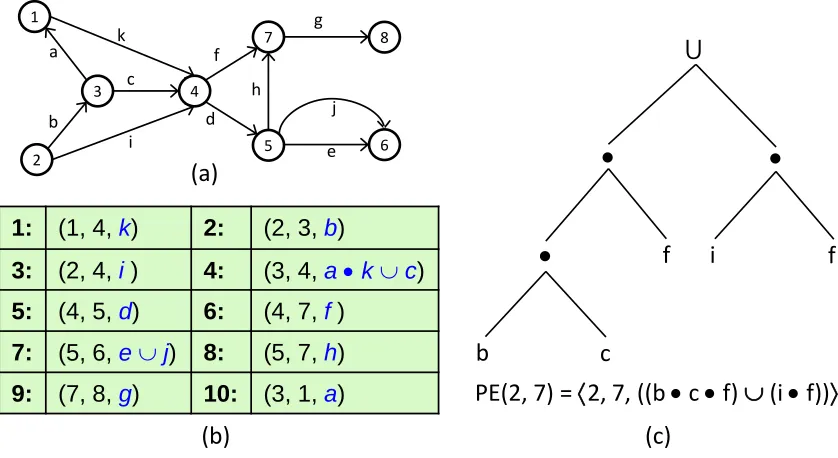
. Let us consider the example graph shown in Figure 3.1(a) which has been borrowed from[GA13a]. Also,λandφdenote empty string and empty set respectively. Now the path expression of type(2,7)
in the example graph would bePE(2, 7)
=
〈2, 7,((b•c•f)∪(i•f))〉1:
(1, 4,
k
)
2:
(2, 3,
b
)
3:
(2, 4,
i
)
4:
(3, 4,
a •
k
c
)
5:
(4, 5,
d
)
6:
(4, 7,
f
)
7:
(5, 6,
e
j
)
8:
(5, 7,
h
)
9:
(7, 8,
g
)
10:
(3, 1,
a
)
⋃
f
b
c
i
f
1: (1, 3, a) 2: (1, 4, k) 3: (2, 3, b) 4: (2, 4, i ) 5: (3, 4, c)
6: (4, 5, d) 7: (4, 7, f ) 8: (5, 6, e) 9: (5, 7, h) 10: (7, 8, g)
(c)
(b)
PE(2, 7) =
2, 7, ((b
•
c
•
f)
(i
•
f))
(a)
1 4 2 3 7 5 8 6 k a b i c d f h g e jFigure 3.1Example graph, Path Expression and Path Sequence
internal nodes while the edges form the leaves of the tree. Figure 3.1(c) shows the AST for the PE shown above.
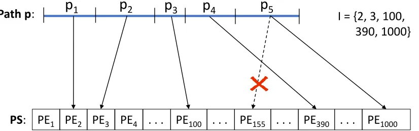
If a graph is ordered using any numbering scheme, information about paths in the graph can be represented using a particular sequence of path expressions called a path sequence (PS)[Tar79b] [GA13a]. A Path Sequence (P S) is a unique ordering of path expressions that represent all path information in a graph, such that for any pathp, there is a unique partition ofp into non empty subpaths, and a unique sequences of indicesI ofP S, such that thei t hsubpath ofpis represented by the path expression inP S at thei t h index inI. Figure 3.1(b) shows the path sequences that represents the example graph in Figure 3.1(a). Figure 3.2 explains the property of Path Sequence that allows the algorithm that uses this construct to solve all paths problem by scanning the path sequence from left to right. Suppose pathp can be divided into 5 subpathsp1,p2,p3,p4,p5and indicesI ={2, 3, 100, 390, 1000}. Then the pathsp1top5must be represented by the path expressions at these indices of the path sequence. However,p5cannot be represented by sayP E155.
Given a path sequence, many path problems can be solved using a simple propagation SOLVE algorithm[Tar79b] [GA13a]that assembles path information as it scans the path sequence from left to right. At every iteration of theSOLVE algorithmthe following step is performed
P E(s,wi)∪(P E(s,vi)•P E(vi,wi))−>S A[wi].
PE
1PE
2PE
3PE
4. . . PE
100. . .
PE
155. . . PE
390. . .
PE
1000PS
:
Path p
:
p
1p
2p
3p
4p
5I = {2, 3, 100,
390, 1000}
Figure 3.2Example explaining Path Sequence
path expression currently inS A[vi], ie,P E(s,vi)by concatenating it withP E(vi,wi)resulting in P E(s,wi). This represents paths fromstowi viavi. This is then used to extend the path expression currently inS A[wi]using union operation resulting in updated path expressionP E(s,wi)which is stored inS A[wi]. This step is performed over and over till the algorithm reaches the end of the path sequence and at the end of the scan, we are guaranteed completeness of the source node used to drive the propagation phase. Figure 3.3 shows a few steps of the SOLVE algorithm with source s =1. Multiple path problems can be solved using the same algorithm by interpreting Union(∪) and concatenation(•) operators appropriately. The same algorithm can be performed for multiple sources to solve path queries with multiple sources and multiple destinations.[GA13a]shows how thisSOLVE algorithmcan be optimized when running for multiple sources such that common paths can be reused instead of being recomputed.
PE(1, 4)
⋃
( )
PE(s, w
i)
⋃
( ) →
SA[w
i]
PE(1, 5)
⋃
( )
Solving(s =1, d):
Initialize: PE(s, s) =
→
SA[s],
PE(s, d) =
for d
≠ 𝑠 →
SA[d]
Step i (iteration i):
PE(s,v
i)
•
PE(v
i,w
i)
Step 1 (s=1, v
1=1, w
1=4):
PE(1,1)
•
PE(1, 4)
=
SA[4]
⋃
(
SA[1]
•
PE(1,4)
)
Step 5 (s=1, v
5=4, w
5=5):
PE(1,4)
•
PE(4, 5)
=
SA[5]
⋃
(
SA[4]
•
PE(4,5)
)
PE(1, 6)
⋃
( )
Step 7 (s=1, v
7=4, w
7=5):
PE(1,5)
•
PE(5, 6)
=
⋃
((k •
d)
•
(e
⋃
j)
= (k •
d •
e)
⋃
(k
•
d •
j)
→
SA[6]
……
……
=
⋃
(
•
k) = k →
SA[4]
=
⋃
(k
•
d) = k •
d →
SA[5]
=
SA[6]
⋃
(
SA[5]
•
PE(5, 6)
)
Figure 3.3Example showing a few steps of the SOLVE algorithm for sources=1
3.2
RDF
The World Wide Web[Www], also known as WWW or simply the Web is a network of informa-tion where each entity, known as resources, is identified by a Uniform Resource Identifiers (URI). This unique identification of each resource facilitates referencing that resource in further build-ing the information network larger by linkbuild-ing each resource to other resources usbuild-ing meanbuild-ingful connections.
The World Wide Web Consortium (W3C)[W3c]is the international standards organization and community that develops and maintains standards for the Web. The Resource Description Framework (RDF)[Rdfb]is a W3C standard model for data on the Web. In the RDF data model two resources identified by their URIs are linked using a predicate. The next subsection discusses the RDF data model in detail.
3.2.1 RDF Data Model
The RDF[Rdfb]data model structures data intotriplesconsisting of asubject,predicateandobject. Now RDF data can also be viewed as graphs where the subject and object are nodes and the predicate is a directed edge from the subject node to the object node. Both these data models are used in this thesis as the pattern matching platform uses the triple data model while the graph processing platform uses the graph data model.
RDF Data Triples RDF Data Triples (Cont.) RDF Data Triples (Cont.)
:prs1 :affWith :u1 :prs3 :affWith :u1 :FP1 :researchInterest “Research1”
:prs1 :affWith :u3 :prs3 :affWith :u4 :Dept1 :name “Dept1” :prs1 :hpage “a.com” :prs3 :affWith :u6 :Dept1 :subOrganizationOf :Univ1 :prs1 :lectures :crs1 :prs3 :mbox “[email protected]” :u1 :name “Univ1” :prs1 :mbox “[email protected]” :prs3 :name “c” :u1 rdf:type :University
:prs1 :name “a” :prs3 :name “cc” …
:prs1 rdf:type :Faculty :prs3 rdf:type :Person RDF Schema Triples
:prs1 rdf:type :Person :prs3 rdf:type :Faculty :lectures rdfs:domain :Faculty
:prs2 :affWith :u1 :crs1 :hpage “crs1.edu” :affWith rdfs:domain :Person :prs2 :affWith :u3 :crs1 :mbox “[email protected]” :affWith rdfs:range xsd:String
:prs2 :affWith :u5 :crs1 :name “crs1” :headOf rdfs:subPropertyOf :worksFor :prs2 :mbox “[email protected]” :crs1 :rating “10” :worksFor rdfs:subPropertyOf :memberOf :prs2 :name “b” :crs1 rdf:type :Course :worksFor rdfs:domain :Employee
:prs2 :name “bb” :FP1 :headOf :Dept1 :Employee rdfs:subClassOf :Person :prs2 rdf:type :Person :FP1 rdf:type :FullProfessor :worksFor rdfs:range :Organization
:prs2 rdf:type :Faculty :FP1 :name “FProf1” :subOrganizationOf rdfs:range :Organization
Figure 3.4RDF Data Model: Table showing example RDF triples
triples in bold and blue. The former capture instance data (assertions about instances of relation-ships or instances of class memberrelation-ships). The latter describes domain concepts, relationrelation-ships and the relationships between them. All the entities that start with ":" have a leading prefix such as 〈
http://swat.cse.lehigh.edu/onto/univ-bench.owl#
〉which has been omitted from the table for brevity. Hence, each entity that starts with ":" is a unique identifiers or URI while each entity that is enclosed in quotes is a string literal.:prs1 :u1
:u3 :crs1
:Faculty
:Person :University
:Dept1
:affWith rdf:type rdf:type
:subOrganizat ionOf
:name
:n
am
e
“Univ1” “a.com”
“a” “[email protected]”
“Dept1”
Figure 3.5RDF Data Model: Triples represented in the form of graph with directed edges
triple〈
:affWith rdfs:range :University
〉denotes that the property:affWith
will always have entities of type:University
as the object, for example〈:prs1 :affWith :u1
〉where〈:u1
rdf:type :University
〉.Figure 3.5 shows the part of the RDF data shown in Figure 3.4 represented as a graph where the subjects and objects like
:prs1
and:u1
respectively are nodes while the predicates like:affWith
are directed and labeled edges between the nodes where the lable of the edge is the predicate itself. Nodes denoted using ovals are resources identified by unique identifiers or URIs and the nodes denoted by rectangular boxes are string literals. Also therdf:type
edges are shown with bold arrows. Although this graph only shows a sample of the data triples, the schema triples can also be denoted in a similar manner. For path computation RDF data is modelled in this way as a graph with directed and labeled edges.3.3
Algebraic Query Evaluation of Graph Pattern Matching
pattern in a SPARQL query is joined to the next triple pattern using a "." at the end of the triple pattern and the join is performed on the common variable between two triple patterns. For example, if the query contains the graph pattern〈
?s :affWith :u1 . ?s :affWith :u3 .
〉then?s
will bind to only{:prs1, :prs2
}. This graph pattern contains a "subject-subject" join since both the triple patterns have the join variable in their subject position. Joins in SPARQL can also be "subject-object" join where one triple pattern has the join variable in the subject position while the other triple pattern. An exmaple of such a join would be the graph pattern〈:prs1 :lectures ?o
. ?o rdf:type :Course .
〉. Here the variable?o
will bind to{:crs1
}. The last type of join in SPARQL is the object-object join, for example, the graph pattern〈:prs1 :affWith ?o . :prs3
:affWith ?o .
〉where the variable?o
would bind to{:u1
}.Evaluation of graph pattern matching query is usually performed using operators with an algebraic query plan where we typically use relational-like query operators. The graph patterns are compiled into an algebraic logical plan representation, which is generally a sequence of query operators with an implied execution ordering. For example, Jena ARQ[McB02][Jen]is a popular query engine that supports SPARQL queries and it creates a SPARQL Syntax-Expression(SSE) as an algebraic logical query plan. The last step in query evaluation is transforming the logical plan to a physical plan which depends on the physical execution environment.
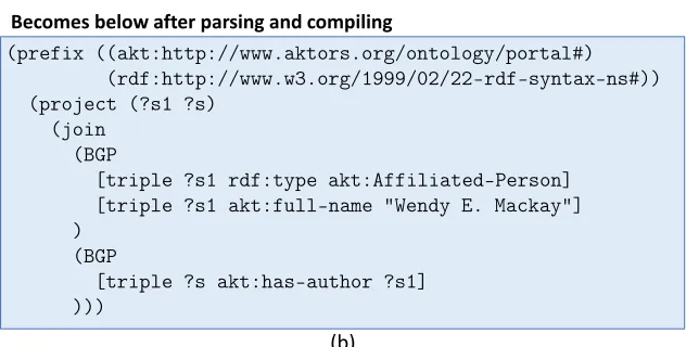
3.3.1 Apache Jena
PREFIX akt:<http://www.aktors.org/ontology/portal#> PREFIX rdf:<http://www.w3.org/1999/02/22-rdf-syntax-ns#>
SELECT * WHERE {
?s1 rdf:type akt:Affiliated-Person . ?s1 akt:full-name "Wendy E. Mackay" . ?s akt:has-author ?s1 .
}
Original Query String
(prefix ((akt:http://www.aktors.org/ontology/portal#) (rdf:http://www.w3.org/1999/02/22-rdf-syntax-ns#)) (project (?s1 ?s)
(join (BGP
[triple ?s1 rdf:type akt:Affiliated-Person] [triple ?s1 akt:full-name "Wendy E. Mackay"] )
(BGP
[triple ?s akt:has-author ?s1] )))
Becomes below after parsing and compiling
(a)
(b)
Figure 3.6Example SPARQL query and its transformation after compilation by Jena’s parser (a) Example query (b) Corresponding SSE
3.4
Semstorm
[Kim17d] [Kim17a]introduces a Hadoop-based file organization that supports efficient storage of data collections. It also supports optimized graph pattern matching queries which are executed in Apache Tez[Tez]environment. Prior to using Semstorm for executing SPARQL queries, a pre-processing step is necessary. This step prepares the dataset for querying by grouping triples in triplegroups. Triples are grouped together based on their subject URI and then these triplegroups are typed based on the specific predicates in each triplegroup. These pre-processed triples are stored in files and these files are later used for querying instead of the actual dataset. This pre-processing step helps in eliminating subject-subject joins during query execution since the data is stored and indexed accordingly, thus, improving the efficiency of Semstorm’s query execution.
3.4.1 Apache Tez
Apache Tez is a framework that can be used by data processing applications in Hadoop. Tez im-proves upon the old MapReduce framework by dramatically improving its speed, while maintaining MapReduce’s ability to scale. Tez provides a simple API to represent data processing steps in the form of a Directed Acyclic Graph (DAG). Each vertex in the DAG defines the logic for data manipulation (for example, filter conditions) and also states the resources and environment required for the logic to be executed (for example, input file or output file location etc). Every vertex is a composition of Logical Input, Logical Output, Processorand an optionalConfiguration payload. Each edge in the DAG defines the flow of data between producer and consumer vertices. During query execution in Tez, the intermediate results are stored in memory and only spills to disk when there is not enough memory to hold the data. Another factor that adds to the efficiency of Apache Tez is the fact that it processes a batch of rows instead of one row at a time.
In the DAG created by Semstorm the leaves are usually the nodes that reads data from HDFS while the root vertex writes output to HDFS. The intermediate vertices are involved in different types of processing steps such as joining, annotating, filtering etc.
3.4.2 Loops and Cycles:
Asimple pathis a path that does not contain any repeated nodes while acycleis an alternating set of nodes and edges (a path) where a node is reachable starting from itself. Now cycles can be of multiple types such as asimple cyclewhere only the starting and ending node can be repeated. A loop[Gui] [BM76](also calledself-loop) can be thought of as a type of cycle with one node and one edge connects the node to itself.
3.5
Serpent
CHAPTER
4
APPROACH
Our approach can be divided into three main phases. 1. Query Expression
Goal:While expressing the gpq our goal was to minimize disruption to existing infrastructure, e.g. parser.
Solution:To achieve this goal we introduced a syntactic sugar to represent the path operator. 2. Query Compilation
Goal:For being able to compile the gpq we need to integrate graph pattern matching with path problem solving.
Solution:We modified the graph pattern matching logical query plan generated by the pattern matching engine by splicing in algebraic path querying operators to produce a gpqs query plan.
3. Query Execution
Goal:The final phase includes executing gpqs.
For implemnting our approach We built a prototype by integrating the graph pattern matching platformSemStormwith path computation platformSerpent. Semstorm is a Hadoop-based file organization storage system that supports efficient graph pattern matching query execution using an algebraic query evaluation technique. Semstorm uses Apache Tez as the execution environment. Serpent is a platform for finding all paths between a set of sources and destinations. It builds on the path algebraic technique using path-sequences to compute paths.
4.1
Query Expression
Introducing a new query class would typically require the extension of query language and process-ing framework. However, we adopted an approach of introducprocess-ing a syntactic sugar that avoided the need for changing SPARQL’s query syntax. This approach also enables us to minimize disruption of existing infrastructure , for example, the parser of the graph pattern matching engine.
Although this approach has a lot of positives it suffers from two main issues. Firstly, since we are not modifying the parser of the pattern matching platform it would not recognize anew path operator in the query syntaxand such a query would fail during compilation. Secondly, the pattern matching platform would produce a graph pattern query plan which we mustmigrateto agpq query plan. Also, we would need to identify the sub-query components, i.e., source variable, destination variable and constraint variable and then project the bindings to these variables while filtering out the bindings to the rest of the variables.
(prefix ((akt:http://www.aktors.org/ontology/portal#) (rdf:http://www.w3.org/1999/02/22-rdf-syntax-ns#)) (project (?s1 ?s)
(product (join
(BGP
[triple ?s1 rdf:type akt:Affiliated-Person] [triple ?s1 akt:full-name "Wendy E. Mackay"]) (BGP
[triple ?s akt:has-author ?s1] ))
(BGP
[triple ?s2 akt:full-name "Irene Greif"] [triple ?s2 akt:has-affiliation ?d]))) SSE produced by Jena after parsing and compiling PREFIX akt:<http://www.aktors.org/ontology/
portal#>
PREFIX rdf:<http://www.w3.org/1999/02/22-rdf-syntax-ns#>
SELECT * WHERE {
?s1 rdf:type akt:Affiliated-Person . ?s1 akt:full-name "Wendy E. Mackay" . ?s akt:has-author ?s1 .
?s2 akt:full-name "Irene Greif" . ?s2 akt:has-affiliation ?d .
?s ?pathVar ?d . }
Original query
(a) (b)
4.1.1 Identifying GPQ Sub-Query Components in SPARQL* Queries:
Our syntactic sugar is based on adopting a pre-defined variable name?pathVaras the path operator. We acknowledge the risk of other users using this variable in their queries, but assume this risk to be small. However, this operator should also be a legal variable that is recognized by the graph pattern matching platform’s parser. This will ensure that the unaltered parser can parse and compile path queries without failing due to syntax issues. Here, we refer to SPARQL with our pre-defined variable ?pathVarasSPARQL*.
4.1.2 Implementation Strategy:
In this section, we describe the approach followed to identify the source and destination variables using the pre-defined path variable?pathVarand then project them out from the graph patterns. Figure 4.1 shows a typical query in our integrated platform and the corresponding SSE produced by Jena’s parser and compiler. The last triple pattern in example query in Figure 4.1(a),〈?s ?pathVar ?d〉 denotes the path computation between all bindings to the variable?sand the variable?d. Presence of the?pathVarvariable in the predicate position implies that it is a path query. Now, we must keep track of the position of the source and destination variables in the graph patterns and finally, after all the joins have taken place we must project out only the bindings of the source and destination variables. These bindings would then go into the path operator. To do this, we create the required datastructures to hold the position information of the source and destination variables in the query. This information will be later required when we create the final physical plan of the query.
For our proof-of-concept prototype, we implemented the approach by integratingSemstorm [Kim17c]as the graph pattern matching platform andSerpent[GA13a][Gao18]as the path query com-putation platform. Semstorm uses the below two main datastructures as query plan representation to hold the position information of the different triple patterns in the submitted query.
• subjObjListMapholds the mapping between the subjects and the corresponding objects in the query. The subjObjListMap for the query in Figure 4.1(a) would be
subjObjListMap: {?s=[[?s1]], ?s1=[["Wendy E. Mackay"]],
?s2=[["Irene Greif"], [?d]]}
• subjPropListMapholds the mapping between the subjects and the properties or predicates in the triple patterns in the query. The subjPropListMap of the query in Figure 4.1(a) would be
In addition to these, the following datastructures have been added to facilitate path computation and provide required location information to the path operator.
• pathSrcDstis a map that shows the mapping between the source variable and its correspond-ing destination variable. For the query in Figure 4.1(a), the pathSrcDst would be
pathSrcDst: {?s=[?d]}
The current structure of this map allows one source variable to have multiple destination variables, since the value in this map is a list of destination variables. However, we have not tested queries with multiple destinations and path operator variables. Some more develop-ment work would be required before our platform can handle multiple path operator variable and we leave that for future work.
• srcMapcontains the source variable in the key position and a list of integers in the value posi-tion. The list of integers denote the exact position of the source variable in the subjObjListMap datastructure. The srcMap of the query in Figure 4.1(a) would be
srcMap: {?s=[[0, -1]]}
• dstMapis similar to the srcMap, except that its key contains the destination variable and the list of integers in its value position denote the position of the destination variable. The dstMap of the query in Figure 4.1(a) would be
dstMap: {?d=[[2, 1]]}
• cndMapis also same as the srcMap and dstMap except that it hold the constraints information. For example, some query might want to restrict paths to the ones which contain at least one akt:has-affiliationproperty or predicate. Then, this triple will be a part of the constraints and the position of this triple would be captured in the cndMap. The query in Figure 4.1(a) is not a constrained query and hence, its cndMap would be empty.
they can exist in multiple BGPs and the value of the respective maps will have a list of integer pairs, identifying the position of the variable in subjObjListMap. The information stored in these new datastructures are used during query evaluation phase later to identify the source, destination and constraint variables and then project only the bindings to these variables while filtering out the rest.
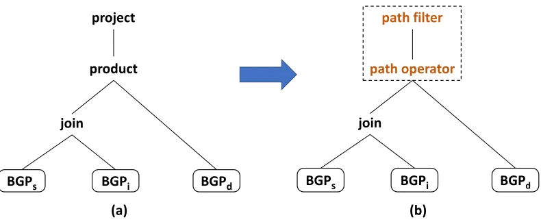
4.2
Query Compilation
Since we are interpreting the problem algebraically it translates to query evaluation being repre-sented by an expression composed of multiple query operators in a specified order. It is easy to observe that gpqs are essentially comprised of four elements:
• Filtering of graph patterns, • Graph pattern matching, • Path finding,
• Path filtering
Figure 4.2 shows these four components and the pieces from the motivating example that correspond to each of these components. An algebraic evaluation of gpqs would involve translating each of these components into one or more query operator and then deciding the most efficient ordering of these operators. Since there are efficient algebraic pattern matching engines available, we can leverage these engines for the first two components. Then we would need to create logical operators to represent the path finder and path filter components.
Path Filter Path Finder
Pattern Filter Pattern
Matching
P1: Passengers on flights to Washington DC, Purchased one-way tickets by cash
P2: Countries on the CIA watchlist
Finding paths between P1 and P2 P1: Between June
30 and July 6
With at least one financial link
Can leverage existing graph pattern matching engines for these.
Need to create logical operators to represent these components
BGPs BGPi BGPd join
product project
BGPs BGPi BGPd
join
path operator path filter
(a) (b)
Figure 4.3Query plan transformation from graph pattern matching query to gpq
4.2.1 Logical Query Plan Transformation:
A simplifying but reasonable strategy to develop the logical query plan is the use of a fixed order between the graph pattern matching phase and the path computation phase. The rationale here is that in gpqs, pattern matching serves to compute the set of sources, destinations and/or intermediate nodes in constraints. In other words, the output of graph pattern matching can be seen as input to the path problem phase. Interpreting this in terms of query plans implies that the path computation and path filter operators will always be at the root of the tree for any gpqs query plans. In the sequel, we elaborate our realization of the above implied strategy.
Our query planning approach is based on transforming the query plan produced by graph pattern matching engine to a generalized path query evaluation plan. The intuition is that the subqueries which are the graph patterns defining the sets of sources, destinations and constraints for path computation can be translated to query plans in the usual manner. However, the semantics of such queries will usually imply a cross-product of intermediate results (since the subgraph patterns will be disconnected). We illustrate this idea with the example query in Figure 4.1(a) (but ignoring the last triple pattern〈
?s ?pathVar ?d
〉which is our syntactic sugar for the path variable triple pattern). 4.1(b) shows the SSE created by Jena’s parser and compiler and Figure 4.3(a) shows the SSE as a tree. Figure 4.3(b) shows the transformed query plan suited for the correspondinggpq.The new components of the query plan are highlighted in orange in Figure 4.3(b). The final operator in the plan is a path filter operator (if path filtering constraints are specified - absent in example). The newly introduced components of the query plan are enclosed in a dotted box in Figure 4.3(b).
4.3
Query Execution
Our graph pattern matching platform, Semstorm[Kim17c]is an RDF processing platform that is targeted for Cloud-processing and uses Apache Hadoop/Tez execution environment. Semstorm’s compiler builds on Jena’s parser, using Jena’s SSE to create a Tez[Tez]DAG as the physical query plan based on Semstorm’s query algebra. To achieve an equivalent physical query plan transformation, similar to the logical plan transformation in Figure 4.3, new physical query operators have to be introduced. Since our physical execution environment is Tez, the new physical operators are nothing but new Tez Vertices.
4.3.1 Implementation Strategy
We introduced four new Tez vertex types were added that act as the physical query operators. • Annotator Vertex for source, destination and constraint variables.Semstorm is meant to
runSELECT * WHEREqueries and so, it propagates the data for all of the variables in the query. Hence, the output of theTypeScannerorPackagervertex contains subjects, predicates and objects that have bound to all the variables in the query. However, the path computation platform Serpent expects three lists of nodes that denote sources, destinations and constraints respectively. Hence, annotators were required to identify the source, destination or constraint variables and then, allow only the bindings for that variable to pass through, discarding the rest of the bindings. While this might seem to be a less optimized method, it must be noted that bindings to other variables cannot be discarded before all joins have completed since the source, destination or constraint variable may not always be the join variable.
• PathComputer Vertex.This is the path operator which performs the path computation. It takes the sources, destinations and constraints as input, converts these into three String arrays as is required by Serpent and then calls the appropriate method in the Serpent platform. For every path query DAG this vertex will always be at the root.
Figure 4.4 shows the final Tez DAG that needs to be generated for the example query in Figure 4.1(a). TheTypeScanner::?svertex in the DAG identifies and reads all triples that match the pattern
TypeScanner:: ?s
TypeScanner:: ?s1 Annotator
-Source: [[0, -1]]
Annotator -Destination: [[2, 1]] PathComputer::
Src: ?s, Dst: ?d
TypeScanner:: ?s2 Packager::
?s,?s1
Annotator (?s1): 0
Annotator (?s1): 1
BGP
d
BGP
i
BGP
s
Figure 4.4The Tez DAG representating the physical plan for the query shown in Figure 4.1(a)
that match the pattern{
?s1 rdf:type akt:Affiliated-Person . ?s1 akt:full-name "
Wendy E. Mackay"
}. TheTypeScanner::?s2vertex reads all graph patterns that match the pattern{?s2 akt: full-name "Irene Greif" . ?s2 akt:has-aff iliation ?d}
. The output of theTypeScanner::?sandTypeScanner::?s1vertices go toAnnotator(?s1):0andAnnotator(?s1):1 ver-tices respectively. These annotator verver-tices identify the join variable and its position in the graph pattern. For example,Annotator(?s1):0identifies?s1
as the join variable and it is at the first position (index starts at 0) in thesubjObjListMap
described earlier. ThePackager::?s,?s1vertex performs the actual join operation between the two graph patterns and provides the joined output of the two input graph patterns.on disk. In our integrated version, we created a fork at this point, where for a path query, we do not add theProducterandFlattenervertices. After joins, we add theAnnotator- Source:[[0,-1]]and Annotator-Destination:[[2,1]]to annotate the source and destination respectively. We also add the value from the
srcMap
anddstMap
to the respective vertex name. Since the destination vertex in our example is not involved in any joins the destination annotator vertex gets its input directly from the typeScanner vertex that has the destination variable. ThePathComputer::Src:?s, Dst:?dvertex comes at the root of the DAG since this will be executed last. While creating this vertex, information about the source variable?s
and destination variable?d
are added to it using the configuration payload. This DAG is submitted to the query execution framework of Semstorm, which executes the DAG and produces the final path output.4.4
Path Constraints
Some path constraints can be evaluated by reinterpreting the union and concatenation operations during the propagation algorithm (SOLVE) e.g. for shortest paths. Others will be defined as manipula-tions over the path expression produced by unconstrained version of the problem e.g. finding paths that contain a given set of nodes (no order specified). Those manipulations will be encapsulated in operators that are parent nodes of the pathComputer node in operator plan tree. The efficiency of the such operations will depend on the nature of path expression representation e.g. a binary encoded representation. However, a detailed discussion path constraints is outside scope of this thesis.
4.5
User Interface Updations:
Semstorm uses a settings file to capture configurations such as input file location, ontology file location and so on. Also, Semstorm requires the user to write the full SPARQL query and create a query file that must be provided as an argument to the Main method when running any queries. To remove this requirement of the user needing to write the full query, we also added a few new fields in thesettings.inifile of the Semstorm platform. The new settings file is shown in below.
[semstorm]
localMode = true
numPartitions = 1
inputPath = src/test/resources/data/btc500M.nt
interimPath = triplegroups
outputPath = queryOutput
yarnResourceMangerPort = 8050
hdfsNamenodePort = 8020
tezCompressFilePath = /hdp/apps/current/tez/tez.tar.gz
SemStormFilePath = /hdp/apps/current/tez/aux-jars/SemStorm.jar
usePropTypeCache = true
prefix = akt:<http://www.aktors.org/ontology/portal#>, rdf:<http:
//www.w3.org/1999/02/22-rdf-syntax-ns#>, acm:<http://acm.rkbexpl
orer.com/ontologies/acm#>, acmper:http://acm.rkbexplorer.com/id/
triplePatterns = ?s1 rdf:type akt:Affiliated-Person , ?s1 akt:fu
ll-name "Wendy E. Mackay" , ?s akt:has-author ?s1 , ?s2 akt:full
-name "Irene Greif" , ?s2 akt:has-affiliation ?d
[serpent]
preprocess = false
inputPath = src/test/resources/data/btc500M.nt
interimPath = pathseqs
nodeTypeMapPath = src/test/resources/nodetypemap.ser
isPathQuery = yes
direction = d
srcVar = ?s
dstVar = ?d
cndVar =
cndTriples =
constOption =
CHAPTER
5
EVALUATION
5.1
Test setup
The primary goal of our evaluation was to compare our integrated system with existing platform that can perform multi-source multi-destination path querying where the source and destination nodes are described as graph patterns on the following parameters.
1. Performance, i.e., time taken to run the same queries.
2. Completeness of results, i.e., whether the platform returns all paths expected. 3. Expressiveness, i.e., what level of queries can be expressed in each platform.
4. Query compilation time comparison on our platform with and without path operator. 5.1.1 Dataset and Queries:
queries we used. In the charts Small Queries and Large Queries have been abbreviated to SQ and LQ respectively due to shortage of space. The same queries were also modified to add constraints to run constrained query experiments.
All the comparisons were done with Stardog. We also considered comparing our platform wit Neo4j. However, while trying to run the queries using Cypher we found that the resources available on our server was not enough to run all-paths queries on the BTC dataset on Neo4j. All-paths queries on this dataset were running indefinitely and then causing the Neo4j server to crash. We were able to run shortest path queries on Neo4j but that result is not included in this thesis as finding shortest path is not an evaluation goal for this thesis.
5.1.2 Hardware Configuration:
Evaluation was conducted on single node running Hadoop in a privately owned RedHat Enterprise Server server housed in the University’s server lab. The server is equipped with Xeon octa core x86_64 CPU (2.33 GHz), 40GB RAM, and two HDDs (3.6TB and 445GB). All results have been averaged over five trials.
5.2
Evaluation Results
In all the charts our platform has been labelled as "Sem-Ser". 5.2.1 Performance Evaluation:
When comparing absolute time taken by our platform with that of Stardog, we found that Stardog performed better in all queries except forSm a l l Q u e r y1,L a r g e Q u e r y1andL a r g e Q u e r y2. The L a r g e Q u e r y2timed out and produced only partial results when run on Stardog. This query took the longest time (5.5 minutes) and produced the largest number of paths (0.8 million paths) in our platform. This is mainly because the graph patterns provided for the source and destination nodes
Number of sources and Destinations
Queries Sources Destinations Queries Sources Destinations
SmallQuery1 25 2 LargeQuery1 13641 907
SmallQuery2 4 6 LargeQuery2 29974 32583 SmallQuery3 4 3 LargeQuery3 11793 6 SmallQuery4 29 7 LargeQuery4 29974 2290 SmallQuery5 26 31 LargeQuery5 2290 32582
Large Queries Number of Paths Comparison
Sem-Ser Stardog
Small Queries Number of Paths Comparison
Sem-Ser Stardog 0 500 1000 1500 2000 2500 3000 SQ2 N u mb er of p at h s 0 50 100 150 200 250 300 350
SQ1 SQ3 SQ4 SQ5
N u mb er of p at h s 0 2000 4000 6000 8000 10000 LQ1 LQ3 N u mb er of p at h s 0 150000 300000 450000 600000 750000 900000
LQ2* LQ4 LQ5
N u mb er of p at h s
(a)
(b)
Figure 5.2Number of paths comparison
is quite general, thus leading to large number of matches. As can be seen from Table 5.1 this query resulted in almost thirty thousand source nodes and over thirty two thousand destination nodes. Consequently there were a large number of paths connecting these nodes.
5.2.2 Completeness of results:
Figure 5.2(a) shows the number of paths identified by small queries and Figure 5.2(b) shows the same for larger queries executed.LQ2has been marked with an asterix since it did not finish in Stardog and hence, all the charts have only one value for this query. For all the queries Stardog produced incomplete results and also duplicate paths. This dataset has a lot of triples such as〈
acm:58567
akt:has-publication-reference acm:58567
〉. In this triple the subject and the object is the same uriacm:58567
and hence this is called alooporself-loop. The BTC dataset has a lot of such triples and Stardog does not consider the self loops in the paths it identifies. For example, suppose we have the RDF graph shown in Figure 5.3 consisting of the following triples〈A p1 A
〉 〈A p2 B
〉 〈B p3 B
〉. Now suppose the source node given to the query isA
and destination node isB
. On path query execution Stardog will ignore the self-loops〈A p1 A
〉and〈B p3 B
〉and will output only one path (A p2 B
). However, our platform will include the self-loops and hence find four paths (A
p2 B
), (A p1 A p2 B
), (A p2 B p3 B
) and (A p1 A p2 B p3 B
). Figure 5.3(b) shows the paths returned by each platform. Using the "CYCLIC" keyword, while running the queries in Stardog,to detect loops also did not work since this keyword is looking for "cycles" and not "loops". Rather than giving the correct number of paths, use of the "CYCLIC" keyword reduced the number of paths to zero (most likely because the source and destination sets were disjoint - hence there were no cycles). This is the reason behind Stardog mostly finding less paths as compared to our platform.A p2 B
p1 p3
Sem-Ser Paths
Stardog Paths
A p2 B
A p2 B
A p1 A p2 B
A p2 B p3 B
A p1 A p2 B p3 B
(a)
(b)
Figure 5.3Explanation of self-loops (a) Example graph (b) Comparison of the paths found by Sem-Ser vs Stardog
produces 40 paths forSm a l l Q u e r y1the number of unique paths is 6. Since there was a big mis-match between the number of paths found by our platform and Stardog we compared the time taken per path identified rather than the absolute time taken for executing each query. Figure 5.4(a) shows the time per path comparison for the small queries and Figure 5.4(b) shows the same for large queries. For some queries, which our platform is better optimized for, the difference in time taken per path was big, while for others the difference is quite small. However, in all of the queries our platform takes less time per path as compared to Stardog.
5.2.3 Expressiveness:
All types of graph patterns can be expressed in Neo4j, Stardog as well as our platform. However, Stardog does not support constraints such asALL, ANY, NONE which can be used to filter out certain paths as required. Figure 5.6 shows the comparison of the expressiveness of our platform with that of Stardog and Neo4j. The "ALL" keyword in Stardog is used to denote all paths. Neo4j
Small Queries time per path
Sem-Ser Stardog 0.00 20.00 40.00 60.00 80.00 100.00 120.00 140.00
SQ2 SQ3 SQ4 SQ5
Tim e p er p at h ( millisecs ) 0.00 300.00 600.00 900.00 1200.00 SQ1 Tim e p er p at h ( millisecs )
Large Queries time per path
Sem-Ser Stardog 0.00 2.00 4.00 6.00 8.00 10.00 12.00
LQ1 LQ3 LQ4
Tim e p er p at h ( millisecs ) 0.00 0.05 0.10 0.15 0.20 0.25 0.30 0.35 0.40 0.45 LQ2* LQ5 Tim e p er p at h ( millisecs )