Contents lists available atScienceDirect
Artificial Intelligence
www.elsevier.com/locate/artint
Itemset mining: A constraint programming perspective
Tias Guns
∗
, Siegfried Nijssen, Luc De Raedt
Katholieke Universiteit Leuven, Celestijnenlaan 200A, 3001 Leuven, Belgium
a r t i c l e
i n f o
a b s t r a c t
Article history: Received 31 May 2010
Received in revised form 5 May 2011 Accepted 6 May 2011
Available online 11 May 2011 Keywords:
Data mining Itemset mining Constraint programming
The field of data mining has become accustomed to specifying constraints on patterns of interest. A large number of systems and techniques has been developed for solving such constraint-based mining problems, especially for mining itemsets. The approach taken in the field of data mining contrasts with the constraint programming principles developed within the artificial intelligence community. While most data mining research focuses on algorithmic issues and aims at developing highly optimized and scalable implementations that are tailored towards specific tasks, constraint programming employs a more declarative approach. The emphasis lies on developing high-level modeling languages and general solvers that specifywhatthe problem is, rather than outlininghow a solution should be computed, yet are powerful enough to be used across a wide variety of applications and application domains.
This paper contributes a declarative constraint programming approach to data mining. More specifically, we show that it is possible to employ off-the-shelf constraint program-ming techniques for modeling and solving a wide variety of constraint-based itemset mining tasks, such as frequent, closed, discriminative, and cost-based itemset mining. In particular, we develop a basic constraint programming model for specifying frequent itemsets and show that this model can easily be extended to realize the other settings. This contrasts with typical procedural data mining systems where the underlying procedures need to be modified in order to accommodate new types of constraint, or novel combinations thereof. Even though the performance of state-of-the-art data mining systems outperforms that of the constraint programming approach on some standard tasks, we also show that there exist problems where the constraint programming approach leads to significant performance improvements over state-of-the-art methods in data mining and as well as to new insights into the underlying data mining problems. Many such insights can be obtained by relating the underlying search algorithms of data mining and constraint programming systems to one another. We discuss a number of interesting new research questions and challenges raised by the declarative constraint programming approach to data mining.
©2011 Elsevier B.V. All rights reserved.
1. Introduction
Itemset mining is probably the best studied problem in the data mining literature. Originally applied in a supermarket setting, it involved finding frequent itemsets, that is, sets of items that are frequently bought together in transactions of customers [1]. The introduction of a wide variety of other constraints and a range of algorithms for solving these constraint-based itemset mining problems [33,5,41,42,11,31,50,9] has enabled the application of itemset mining to numerous other
*
Corresponding author. Tel.: +32 16 32 75 67; fax: +32 16 32 79 96. E-mail address:[email protected](T. Guns).0004-3702/$ – see front matter ©2011 Elsevier B.V. All rights reserved. doi:10.1016/j.artint.2011.05.002
problems, ranging from web mining to bioinformatics [31]; for instance, whereas early itemset mining algorithms focused on finding itemsets in unsupervised, sparse data, nowadays closed itemset mining algorithms enable the application of itemset mining on dense data [40,43], while discriminative itemset mining algorithms allow for their application on su-pervised data [35,13]. This progress has resulted in many effective and scalable itemset mining systems and algorithms, usually optimized to specific tasks and constraints. This procedural and algorithmic focus can make it non-trivial to extend such systems to accommodate new constraints or combinations thereof. The need to allow user-specified combinations of constraints is recognized in the data mining community, as witnessed by the development of a theoretical framework based on (anti-)monotonicity[33,41,11] and systems such as ConQueSt [9], MusicDFS [50] and Molfea [18]. These systems support a predefined number of (anti-)monotonicity based constraints, making them well suited for a number of typical data mining tasks.
These approaches contrast with those of constraint programming. Constraint programming is a general declarative methodology for solving constraint satisfaction problems, meaning that constraint programs specify whatthe problem is, rather than outlinehowthe solution should be computed; it does not focus on a particular application. Constraint program-ming systems provide declarative modeling languages in which many types of constraints can be expressed and combined; they often support a much wider range of constraints than more specialized systems such as satisfiability (SAT) and integer linear programming (ILP) solvers [10]. To realize this, themodelis separated as much as possible from thesolver. In the past two decades, constraint programming has developed expressive high-level modeling languages as well as solvers that are powerful enough to be used across a wide variety of applications and domains such as scheduling and planning [45].
The question that arises in this context is whether these constraint programming principles can also be applied to itemset mining. As compared to the more traditional constraint-based mining approach, this approach would specify data mining models using general and declarative constraint satisfaction primitives, instead of specialized primitives; this should make it easy to incorporate new constraints and combinations thereof as – in principle – only the model needs to be extended to specify the problem and general purpose solvers can be used for computing solutions.
The contribution of this article is that we answer the above question positively by showing that the general, off-the-shelf constraint programming methodology can indeed be applied to the specific problems of constraint-based itemset mining.1 We show how a wide variety of itemset mining problems (such as frequent, closed and cost-based) can be modeled in a constraint programming language and that general purpose out-of-the-box constraint programming systems can effectively deal with these problems.
While frequent, closed and cost-based itemset mining are ideal cases, for which the existing constraint programming modeling language used suffices to tackle the problems, this cannot be expected in all cases. Indeed, in our formulation of discriminative itemset mining, we introduce a novel primitive by means of aglobal constraint. This is common practice in constraint programming, and the identification and study of global constraints that can effectively solve specific subproblems has become a branch of research on its own [6]. Here, we have exploited the ability of constraint programming to serve as an integration platform, allowing for the free combination of new primitives with existing ones. This property allows to find closed discriminative itemsets effectively, as well as discriminative patterns adhering to any other constraint(s). Furthermore, casting the problem within a constraint programming setting also provides us with new insights in how to solve discriminative pattern mining problems that lead to important performance improvements over state-of-the-art discriminative data mining systems.
A final contribution is that we compare the resulting declarative constraint programming framework to well-known state-of-the-art algorithms in data mining. It should be realized that any such comparison is difficult to perform; this already holds when comparing different data mining (resp. constraint programming) systems to one another. In our com-parison we focus on high-level concepts rather than on specific implementation issues. Nevertheless, we demonstrate the feasibility of our approach using our CP4IM implementation that employs the state-of-the-art constraint programming li-brary Gecode [47], which was developed for solving general constraint satisfaction problems. While our analysis reveals some weaknesses when applying this particular library to some itemset mining problem, it also reveals that Gecode can already outperform state-of-the-art data mining systems on some tasks. Although outside the scope of the present paper, it is an interesting topic of ongoing research [37] to optimize constraint programming systems for use in data mining.
The article is organized as follows. Section 2 provides an introduction to the main principles of constraint programming. Section 3 introduces the basic problem of frequent itemset mining and discusses how this problem can be addressed us-ing constraint programmus-ing techniques. The followus-ing sections then show how alternative itemset minus-ing constraints and problems can be dealt with using constraint programming: Section 4 studies closed itemset mining, Section 5 considers discriminative itemset mining, and Section 6 shows that the typical monotonicity-based problems studied in the literature can also be addressed in the constraint programming framework. We also study in these sections how the search of the constraint programming approach compares to that of the more specialized approaches. The CP4IM approach is then evalu-ated in Section 7, which provides an overview of the choices made when modeling frequent itemset mining in a concrete constraint programming system and compares the performance of this constraint programming system to specialized data mining systems. Finally, Section 8 concludes.
1 We studied this problem in two conference papers [16,38] and brought it to the attention of the AI community [17]. This article extends these earlier papers with proofs, experiments and comprehensive comparisons with related work in the literature.
2. Constraint programming
In this section we provide a brief summary of the most common approach to constraint programming. More details can be found in text books [45,3]; we focus on high-level principles and omit implementation issues.
Constraint programming (CP) is a declarative programming paradigm: the user specifies a problem in terms of its con-straints, and the system is responsible for finding solutions that adhere to the constraints. The class of problems that constraint programming systems focus on are constraint satisfaction problems.
Definition 1(Constraint Satisfaction Problem (CSP)).A CSP
P
=
(
V
,
D,
C
)
is specified by•
a finite set of variablesV
;•
an initial domainD, which maps every variablev∈
V
to a set of possible valuesD(
v);
•
a finite set of constraintsC
.A variablex
∈
V
is calledfixedif|
D(
x)
| =
1; a domainD isfixedif all its variables are fixed,∀
x∈
V
:|
D(
x)
| =
1. A domainD is calledstrongerthan domain D ifD(
x)
⊆
D(
x)
for allx∈
V
; a domain isfalseif there exists anx∈
V
such that D(
x)
= ∅
. Aconstraint C(
x1, . . . ,
xk)
∈
C
is an arbitrary boolean function on variables{
x1, . . . ,
xk} ⊆
V
.A solution to a CSP is a fixed domainDstronger than the initial domainD that satisfies all constraints. Abusing notation for a fixed domain, we must have that
∀
C(
x1, . . . ,
xk)
∈
C
:C(
D(
x1), . . . ,
D(
xk))
=
true.A distinguishing feature of CP is that it does not focus on a specific set of constraint types. Instead it provides general principles for solving problems with any type of variable or constraint. This sets it apart from satisfiability (SAT) solving, which focuses mainly on boolean formulas, and from integer linear programming (ILP), which focuses on linear constraints on integer variables.
Example 1.Assume we have four people that we want to allocate to two offices, and that every person has a list of other
people that he does not want to share an office with. Furthermore, every person has identified rooms he does not want to occupy. We can represent an instance of this problem with four variables which represent the persons, and inequality constraints which encode the room-sharing constraints:
D
(
x1)
=
D(
x2)
=
D(
x3)
=
D(
x4)
= {
1,
2},
C
= {
x1=
2,
x1=
x2,
x3=
x4}
.
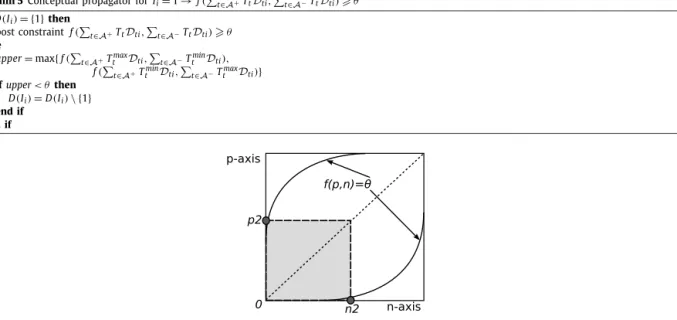
The simplest algorithm to solve CSPs enumerates all possible fixed domains, and evaluates all constraints on each of these domains; clearly this approach is inefficient. Most CP systems perform a more intelligent type of depth-first search, as given in Algorithm 1 [47,45]:
Algorithm 1Constraint-Search(D) 1:D:=propagate(D)
2:ifDis a false domainthen
3: return 4:end if 5:if∃x∈V:|D(x)|>1then 6: x:=arg minx∈V,D(x)>1f(x) 7: for alld∈D(x)do 8: Constraint-Search(D∪ {x→ {d}}) 9: end for 10:else 11: Output solution 12:end if
Other search strategies have been investigated as well [53,44], but we restrict ourselves here to the most common case. In each node of the search tree the algorithm branches by restricting the domain of one of the variables not yet fixed (line 7 in Algorithm 1). It backtracks when a violation of a constraint is found (line 2). The search is further optimized by carefully choosing the variable that is fixed next (line 6); here a function f
(
x)
ranks variables, for instance, by determining which variable is involved in the highest number of constraints.The main concept used to speed up the search is constraint propagation (line 1). Propagation reduces the domains of variables such that the domain remains locally consistent. One can define many types of local consistencies, such as node consistency, arc consistency and path consistency; see [45]. In general, in a locally consistent domain, a valueddoes not occur in the domain of a variable xif it can be determined that there is no solution D in which D
(
x)
= {
d}
. The mainmotivation for maintaining local consistencies is to ensure that the backtracking search does not unnecessarily branch over such values, thereby significantly speeding up the search.
To maintain local consistencies,propagatorsor propagation rules are used. Each constraint is implemented by a propaga-tor. Such a propagator is activated when the domain of one of the variables of the constraint changes. A propagator takes the domain as input and outputs a failed domain in case the constraint can no longer be satisfied, i.e. if there exists no
fixedDstronger thanDwithC
D(
x1), . . . ,
D(
xk)
=
true.
(1)When possible, the propagator will remove values from the domain that can never satisfy the constraint, giving as output a stronger, locally consistent domain. More formally, a value cshould be removed from the domain of a variable
˜
xif there is nofixedDstronger thanDwithD
(˜
x)
=
candCD(
x1), . . . ,
D(
xk)
=
true.
(2)This is referred to as propagation; propagation ensuresdomain consistency. The repeated application of propagators can lead to increasingly stronger domains. Propagators are repeatedly applied until afixed pointis reached in which the domain does not change any more.
Consider the constraintx1
=
x2, the corresponding propagator is given in Algorithm 2:Algorithm 2Conceptual propagator forx1=x2 1:if|D(x1)| =1then 2: D(x2)=D(x2)\D(x1) 3:end if 4:if|D(x2)| =1then 5: D(x1)=D(x1)\D(x2) 6:end if
The propagator can only propagate when x1 orx2 is fixed (lines 1 and 4). If one of them is, its value is removed from the domain of the other variable (lines 2 and 5). In this propagator there is no need to explicitly check whether the constraint is violated, as a violation results in an empty and thus false domain in line 2.
Example 2 (Example 1 continued). The initial domain of this problem is not consistent: the constraint x1
=
2 cannot besatisfied when D
(
x1)
= {
2}
so value 2 is removed from the domain of x1. Subsequently, the propagator for the constraintx1
=
x2 is activated, which removes value 1 fromD(
x2). At this point, we obtain a fixed point with
D(
x1)
= {
1}
,D(
x2)
= {
2}
,D
(
x3)
=
D(
x4)
= {
1,2}
. Persons 1 and 2 have now each been allocated to an office, and two rooms are possible for persons 3 and 4. The search branches over x3 and for each branch, constraint x3=
x4 is propagated; a fixed point is then reached in which every variable is fixed, and a solution is found.In the above example for every variable its entire domain D
(
x)
is maintained. In constraint programming many types of consistency and algorithms for maintaining consistency have been studied. A popular type of consistency is bound con-sistency. In this case, for each variable only a lower- and an upper-bound on the values in its domain is maintained. A propagator will try to narrow the domain of a variable to that range of values for which it still believes a solution can be found, but does not maintain consistency for individual values. To formulate itemset mining problems as constraint programming models, we mostly use variables with binary domains, i.e. D(
x)
= {
0,1}
withx∈
V
. For such variables there is no difference between bound and domain consistency.Furthermore, we make extensive use of two types of constraints over boolean variables, namely thesummation constraint, Eq. (3), andreified summation constraint, Eq. (6), which are introduced below.
2.1. Summation constraint
Given a set of variables V
⊆
V
and weights wxfor each variablex∈
V, the general form of the summation constraint is:x∈V
wxx
θ.
(3)The first task of the propagator is to discover as early as possible whether the constraint is violated. To this aim, the propagator needs to determine whether the upper-bound of the sum is still above the required threshold; filling in the constraint of Eq. (1), this means we need to check whether:
max
fixedDstronger thanD x∈V
wxD
(
x)
A more intelligent method to evaluate this property works as follows. We denote the maximum value of a variablexby xmax
=
maxd∈D(x)d, and the minimum value byxmin
=
mind∈D(x)d. Denoting the set of variables with a positive, respectively negative, weight byV+= {
x∈
V|
wx0}
andV−= {
x∈
V|
wx<
0}
, the bounds of the sum are now defined as:max x∈V wxx
=
x∈V+ wxxmax+
x∈V− wxxmin,
min x∈V wxx=
x∈V+ wxxmin+
x∈V− wxxmax.
These bounds allow one to determine whether an inequality constraintx∈Vwxxθ
can still be satisfied.The second task of the propagator is to maintain the bounds of the variables in the constraint, which in this case are the variables in V. In general, for every variablex
˜
∈
V, we need to updatex˜
minto the lowest valuec for which there exists a domainDwithfixedDstronger thanD
,
D(˜
x)
=
c andx∈V
wxD
(
x)
θ.
(5)Also this can be computed efficiently; essentially, for binary variablesx
∈
V we can update all domains as follows:•
D(
x)
←
D(
x)
\ {
0}
ifwx∈
V+andθ
max(x∈Vwxx
) < θ
+
wx;•
D(
x)
←
D(
x)
\ {
1}
ifwx∈
V−andθ
max(x∈Vwxx) < θ
−
wx.Example 3.Let us illustrate the propagation of the summation constraint. Given
D
(
x1)
= {
1},
D(
x2)
=
D(
x3)
= {
0,
1},
2
∗
x1+
4∗
x2+
8∗
x33;
we know that at least one of x2 and x3 must have value 1, but we cannot conclude that either one of these variables is certainly zero or one. The propagator does not change any domains. On the other hand, given
D
(
x1)
= {
1}
,
D(
x2)
=
D(
x3)
= {
0,
1}
,
2
∗
x1+
4∗
x2+
8∗
x37;
the propagator determines that the constraint can never be satisfied ifx3 is false, soD
(
x3)
= {
1}
.2.2. Reified summation constraint
The second type of constraints we will use extensively is the reified summation constraint. Reified constraints are a common construct in constraint programming [52,54]. Essentially, a reified constraint binds the truth value of a constraint C to a binary variableb:
b
↔
C.
In principle,Ccan be any boolean constraint. In this article,C will usually be a constraint on a sum. In this case we speak of areified summation constraint:
b
↔
x∈V
wxx
θ.
(6)This constraint states that b is true if and only if the weighted sum of the variables in V is higher than
θ. The most
important constraint propagation that occurs for this constraint is the one that updates the domain of variableb. Essentially, the domain of this variable is updated as follows:•
D(
b)
←
D(
b)
\ {
1}
if max(x∈Vwxx) < θ;
•
D(
b)
←
D(
b)
\ {
0}
if min(x∈Vwxx)
θ.
In addition, in some constraint programming systems, constraint propagators can also simplify constraints. In this case, if D
(
b)
= {
1}
, the reified constraint can be simplified to the constraintx∈Vwxxθ
; if D(
b)
= {
0}
, the simplified constraint becomesx∈Vwxx< θ.
Many different constraint programming systems exist. They differ in the types of variables they support, the constraints they implement, the way backtracking is handled and the data structures that are used to store constraints and propagators. Furthermore, in some systems constraints are specified in logic (for instance, in the constraint logic programming system ECLiPSe [3]), while in others the declarative primitives are embedded in an imperative programming language. An example of the latter is Gecode [47], which we use in the experimental section of this article.
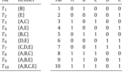
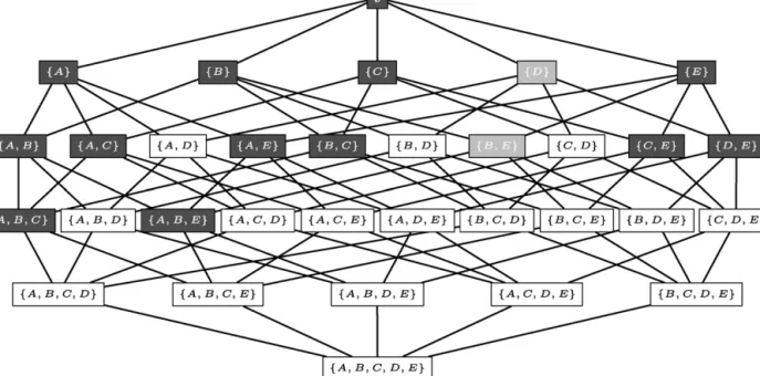
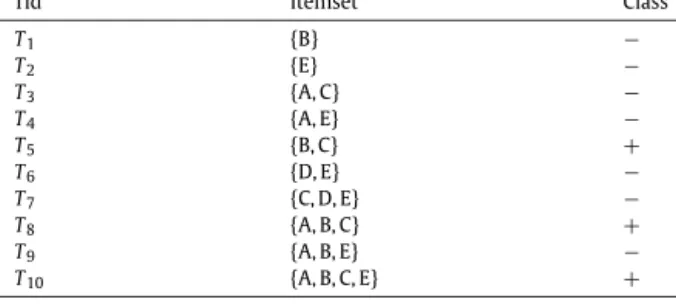
Tid Itemset T1 {B} T2 {E} T3 {A,C} T4 {A,E} T5 {B,C} T6 {D,E} T7 {C,D,E} T8 {A,B,C} T9 {A,B,E} T10 {A,B,C,E} Tid A B C D E 1 0 1 0 0 0 2 0 0 0 0 1 3 1 0 1 0 0 4 1 0 0 0 1 5 0 1 1 0 0 6 0 0 0 1 1 7 0 0 1 1 1 8 1 1 1 0 0 9 1 1 0 0 1 10 1 1 1 0 1
Fig. 1.A small example of an itemset database, in multiset notation (left) and in binary matrix notation (right).
3. Frequent itemset mining
Now that we have introduced the key concepts underlying constraint programming (CP), we study various itemset mining problems within this framework. We start with frequent itemset mining in the present section, and then discuss closed, discriminative andcost-based itemset mining in the following sections. For every problem, we provide a formal definition, then introduce a constraint programming model that shows how the itemset mining problem can be formalized as a CP problem, and then compare the search strategy obtained by the constraint programming approach to that of existing itemset mining algorithms.
We start with the problem of frequent itemset mining and we formulate two CP models for this case. The difference between the initial model and the improved one is that the later uses the notion ofreifiedconstraints, which yields better propagation as shown by an analysis of the resulting search strategies.
3.1. Problem definition
The problem of frequent itemset mining was proposed in 1993 by Agrawal et al. [1]. Given is a database with a set of transactions.2Let
I
= {
1, . . . ,m}
be a set of items andA
= {
1, . . . ,n}
be a set of transaction identifiers. An itemset databaseD
is as a binary matrix of sizen×
mwithD
ti∈ {
0,1}
, or, equivalently, a multi-set of itemsets I⊆
I
, such thatD
=
(
t,
I)
t
∈
A
,
I⊆
I
,
∀
i∈
I:D
ti=
1.
A small example of an itemset database is given in Fig. 1, where for convenience every item is represented as a letter. There are many databases that can be converted into an itemset database. The traditional example is a supermarket database, in which each transaction corresponds to a customer and every item in the transaction to a product bought by the customer. Attribute–value tables can be converted into an itemset database as well. For categorical data, every attribute– value pair corresponds to an item and every row is converted into a transaction.
The coverage
ϕ
D(
I)
of an itemsetI consists of all transactions in which the itemset occurs:ϕ
D(
I)
= {
t∈
A
| ∀
i∈
I:D
ti=
1}
.
Thesupportof an itemset I, which is denoted assupportD
(
I), is the size of the coverage:
supportD
(
I)
=
ϕ
D(
I)
.
In the example database we have
ϕ
D(
{
D,
E}
)
= {
T6,
T7}
andsupportD(
{
D,
E}
)
= |{
T6,
T7}| =
2.Definition 2(Frequent itemset mining).Given an itemset database
D
and a thresholdθ
, the frequent itemset mining problemconsists of computing the set
I
I
⊆
I
,
supportD(
I)
θ
.
The threshold
θ
is called theminimum supportthreshold. An itemset withsupportD(
I)
θ
is called afrequent itemset. Note that we are interested in findingallitemsets satisfying the frequency constraint.The subset relation between itemsets defines a partial order. This is illustrated in Fig. 2 for the example database of Fig. 1; the frequent itemsets are visualized in a Hasse diagram: a line is drawn between two itemsetsI1 and I2 iff I1
⊂
I2 and|
I2| = |
I1| +
1.By changing the support threshold, an analyst can influence the number of patterns that is returned by the data mining system: the lower the support threshold, the larger the number of frequent patterns.
Fig. 2.A visualization of the search space for the database of Fig. 1; frequent itemsets forθ=2 are highlighted. Frequent closed itemsets are highlighted black; non-closed frequent itemsets are grey.
3.2. Initial constraint programming model
Our model of the frequent itemset mining problem in constraint programming is based on the observation that we can formalize the frequent itemset mining problem also as finding the set:
(
I,
T)
I
⊆
I
,
T⊆
A
,
T=
ϕ
D(
I),
|
T|
θ
.
Here we make the set of transactionsT
=
ϕ
D(
I)
explicit. This yields the same solutions as the original problem because the set of transactionsT is completely determined by the itemsetI. We will refer toT=
ϕ
D(
I)
as thecoverage constraintwhile|
T|
θ
expresses asupport constraint.To model this formalization in CP, we need to represent the set of itemsI and the set of transactions T. In our model we use a boolean variable Ii for every individual itemi; furthermore we use a boolean variable Tt for every transactiont. An itemset Iis represented by setting Ii
=
1 for alli∈
I andIi=
0 for alli∈
/
I. The variablesTt represent the transactions that are covered by the itemset, i.e.T=
ϕ
(
I);
Tt=
1 ifft∈
ϕ
(
I). One assignment of values to all
IiandTt corresponds to one itemset and its corresponding transaction set.We now show that the coverage constraint can be formulated as follows.
Property 1(Coverage constraint). Given a database
D
, an itemset I and a transaction set T , thenT
=
ϕ
D(
I)
⇐⇒
∀
t∈
A
: Tt=
1↔
i∈I Ii(
1−
D
ti)
=
0,
(7) or equivalently, T=
ϕ
D(
I)
⇐⇒
∀
t∈
A
: Tt=
1↔
i∈ID
ti=
1∨
Ii=
0,
(8)where Ii
,
Tt∈ {
0,1}
and Ii=
1iff i∈
I and Tt=
1iff t∈
T .Proof. Essentially, the constraint states that for one transactiont, all items i should either be included in the transaction
(
D
ti=
1)or not be included in the itemset(
Ii=
0):T
=
ϕ
D(
I)
= {
t∈
A
| ∀
i∈
I:D
ti=
1}
⇐⇒ ∀
t∈
A
: Tt=
1↔ ∀
i∈
I:D
ti=
1⇐⇒ ∀
t∈
A
: Tt=
1↔
i∈I
Ii
(
1−
D
ti)
=
0.
The representation as a clause in Eq. (8) follows from this.2
It is quite common in constraint programming to encounter different ways to model the same problem or even the same conceptual constraint, as above. How propagation is implemented for these constraints can change from solver to solver. For example,watched literalscould be used for the clause constraint, leading to different runtime and memory characteristics compared to a setting where no watched literals are used. We defer the study of such characteristics to Section 7.
Under the coverage constraint, a transaction variable will only be true if the corresponding transaction covers the itemset. Counting the frequency of the itemset can now be achieved by counting the number of transactions for whichTt
=
1.Property 2(Frequency constraint). Given a database
D
, a transaction set T and a thresholdθ
, then|
T|
θ
⇐⇒
t∈A
Tt
θ,
(9)where Tt
∈ {
0,1}
and Tt=
1iff t∈
T .We can now model the frequent itemset mining problem as a combination of the coverage constraint (7) and the fre-quency constraint (9). To illustrate this, we provide an example of our model in the Essence’ language in Algorithm 3:
Algorithm 3Fim_cp’s frequent itemset mining model, in Essence’ 1:givenNrT, NrI : int
2:givenTDB : matrix indexed by [int(1..NrT),int(1..NrI)] of int(0..1) 3:givenFreq : int
4:findItems: matrix indexed by [int(1..NrI)] of bool 5:findTrans: matrix indexed by [int(1..NrT)] of bool 6:such that
7:$ Coverage Constraint (Eq. (7)) 8:forallt: int(1..NrT).
9: Trans[t]<=>((sum i: int(1..NrI). (1-TDB[t,i])∗Items[i])<=0), 10: $ Frequency Constraint (Eq. (9))
11: (sum t: int(1..NrT).Trans[t])>=Freq.
Essence’ is a solver-independent modeling language; it was developed to support intuitive modeling, abstracting away from the underlying solver technology [22].
We will now study how a constraint programming solver will search for the solutions given the above model. A first observation is that the set of transactions is completely determined by the itemset, so we need only to search over the item variables.
When an item variable is set
(
D(
Ii)
= {
1}
)
by the search, only the constraints that contain this item will be activated. In other words, the frequency constraint will not be activated, but every coverage constraint that contains this item will be. A coverage constraint is areified summation constraint, for which the propagator was explained in Section 2. In summary, when an item variable is set, the following propagation is possible for the coverage constraint:•
if for somet:i∈I(1
−
D
ti)
∗
Imini>
0 then remove 1 from D(
Tt);
•
if for somet:i∈I(1
−
D
ti)
∗
Imaxi=
0 then remove 0 fromD(
Tt).
Once the domain of a variable Tt is changed, the support constraint will be activated. The support constraint is asummation constraint, which will check whether:
t∈A
Ttmax
θ.
If this constraint fails, we do not need to branch further and we can backtrack.
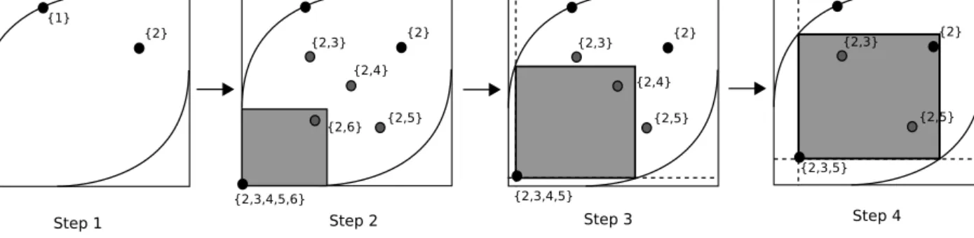
Example 4.Fig. 3(a) shows part of a search tree for a small example with a minimum frequency threshold of 2. Essentially,
the search first tries to add an item to an itemset and after backtracking it will only consider itemsets not including it. After a search step (indicated in green), the propagators are activated. The coverage propagators can set transactions to 0 or 1, while the frequency constraint can cause failure when the desired frequency can no longer be obtained (indicated by a red cross in the two left-most branches).
Fig. 3.Search-propagation interaction of the non-reified frequent itemset model (left) and the reified frequent itemset model (right). A propagation step is colored in blue, a search step in green. (For interpretation of the references to color in this figure legend, the reader is referred to the web version of this article.)
Observe that in the example we branched on item 2 first. This follows the generic ‘most constrained’ variable order heuristic, which branches over the variable contained in most constraints first (remember that the coverage constraints are posted on items that have a 0 in the matrix). If item 1 would be branched over first, the search tree would be larger, as both branches would have to determine separately that I2
=
1 does not result in a frequent itemset. An experimental investigation of different branching heuristics is done in Section 7.3.3. Improved model
Inspired by observations in traditional itemset mining algorithms, we propose an alternative model that substantially reduces the size of the search tree by introducing fine-grained constraints. The main observation is that we can formulate the frequency constraint on each item individually:
Property 3(Reified frequency constraint). Given a database
D
, an itemset I= ∅
and a transaction set T , such that T=
ϕ
D(
I)
, then|
T|
θ
⇐⇒ ∀
i∈
I
:
Ii=
1→
t∈A
Tt
D
tiθ,
(10)where Ii
,
Tt∈ {
0,1}
and Ii=
1iff i∈
I and Tt=
1iff t∈
T .Proof. We observe that we can rewrite
ϕ
D(
I)
as follows:ϕ
D(
I)
= {
t∈
A
| ∀
i∈
I:D
ti=
1} =
i∈I
ϕ
D{
i}
.
Using this observation, it follows that:
|
T|
θ
⇐⇒
j∈I
ϕ
D{
j}
θ
⇐⇒ ∀
i∈
I:ϕ
D{
i}
∩
j∈Iϕ
D{
j}
θ
⇐⇒ ∀
i∈
I:ϕ
D{
i}
∩
Tθ
⇐⇒ ∀
i∈
I
: Ii=
1→
t∈A TtD
tiθ.
2
The improved model consists of the coverage constraint (Eq. (7)) and the newly introduced reified frequency constraint (Eq. (10)). This model is equivalent to the original model, and also finds all frequent itemsets.
The reified frequency constraint is posted on every item separately, resulting in more fine-grained search-propagation interactions. Essentially, the reified frequency constraint performs a kind of look-ahead; for each item, a propagator will check whether that item is still frequent given the current itemset. If it is not, it will be removed from further consideration, as its inclusion would make the itemset infrequent. In summary, the main additional propagation allowed by the reified constraint is the following:
•
if for somei:t∈AD
ti∗
Ttmax< θ
then remove 1 fromD(
Ii), i.e.
Ii=
0.Example 5. Fig. 3 shows the search trees of both the original non-reified model as well as the improved model using the
reified frequency constraint.
In the original model (Fig. 3(a)), the search branches over I2
=
1, after which the propagation detects that this makes the itemset infrequent and fails (left-most branch). In the reified model (Fig. 3(b)) the reified frequency propagator for I2 detects that this item is infrequent. When evaluating the sum(0
∗
Tmax1+
1∗
T2max+
0∗
T3max), it is easy to see that the
maximum is 1<
2, leading to I2=
0 (second level). The same situation occurs for I3 near the bottom of the figure. This time, the propagator takes into account that at this point T3=
0 and henceT3max=
0.The reified propagations avoid creating branches that can only fail. In fact, using the reified model, the search becomes failure-free: every branch will lead to a solution, namely a frequent itemset. This comes at the cost of a larger number of propagations. In Section 7 we experimentally investigate the difference in efficiency between the two formulations.
3.4. Comparison
Let us now study how the proposed CP-based approach compares to traditional itemset mining algorithms. In order to understand this relationship, let us first provide a short introduction to these traditional algorithms.
The most important property exploited in traditional algorithms isanti-monotonicity.
Definition 3(Anti-monotonic constraints). Assume given two itemsets I1 and I2, and a predicate p
(
I,
D
)
expressing acon-straint that itemsetIshould satisfy on database
D
. Then the constraint is anti-monotonic iff∀
I1⊆
I2:
p(
I2,
D
)
⇒
p(
I1,
D
).
Indeed, if an itemset I2 is frequent, any itemset I1⊆
I2 is also frequent, as it must be included in at least the same transactions asI2. This property allows one to develop search algorithms that do not need to consider all possible itemsets. Essentially, no itemset I2⊃
I1 needs to be considered any more once it has been found thatI1is infrequent.Starting a search from the empty itemset, there are many ways in which one could traverse the search space, the most important ones being first search and depth-first search. Initial algorithms for itemset mining were mostly breadth-first search algorithms, of which the Apriori algorithm is the main representative [2]. However, more recent algorithms
mostly use depth-first search. Given that most CP systems also perform depth-first search, the similarities between CP and depth-first itemset mining algorithms are much larger than between CP and breadth-first mining algorithms. An outline of a general depth-first frequent itemset mining algorithm is given in Algorithm 4. The main observations are the following:
•
if an item is infrequent in a database, we can remove the corresponding column from the database, as no itemset will contain this item and hence the column is redundant;•
once an item is added to an itemset, all transactions not containing this item become irrelevant for the search tree below this itemset; hence we can remove the corresponding row from the database.The resulting database, which contains a smaller number of transactions having a smaller number of items, is often called a projected database. Hence, every time that we add an item to an itemset, we determine which items and transactions become irrelevant, and continue the search for the resulting database, which only contains frequent items and transactions covered by the current itemset. Important benefits are that the search procedure will never try to add items once they have been found to be infrequent; transactions no longer relevant can similarly be ignored.
Please note the following detail: in the projected database, we only include items which are strictly higher in order than the highest item currently in the itemset. The reason for this is that we wish to avoid that the same itemset is found multiple times; for instance, we wish to find itemset
{
1,2}
only as a child of itemset{
1}
and not also as a child of itemset{
2}
.Algorithm 4Depth-First-Search (ItemsetI, DatabaseD) 1:F:= {I}
2: determine a total orderRon the items inD
3:for allitemsioccurring inDdo
4: create fromDprojected databaseDi, containing: 5: - only transactions inDthat containi
6: - only items inDithat are frequent and higher thaniin chosen orderR 7: F:=F∪Depth-First-Search(I∪ {i},Di);
8:end for
9: returnF
An important choice in this general algorithm is how the projected databases are stored. A very large number of strate-gies have been explored, among which tid-lists and FP-trees [30]. Tid-lists are most relevant here, as they compare best to strategies chosen in CP systems. Given an itemi, its tid-list in a database
D
isϕ
D(
{
i}
). We can store this list as a list of
integers [56], a binary vector, or using variations of run-length encoding [49]. The projected database of a given itemsetIis thus the seti
,
ϕ
DI∪ {
i}
ϕ
DI∪ {
i}
θ
.
The interesting property of tid-lists is that they can easily be updated incrementally: if we wish to obtain a tid-list for item j in the projected database of itemset
{
i}
, this can be obtained by computingϕ
D(
{
i}
)
∩
ϕ
D(
{
j}
), where
D
is the original database; for instance, in the case bit vectors are used this is a binary AND operation, which most CPUs evaluate efficiently. The most well-known algorithm using this approach is the Eclat algorithm [56].An example of a depth-first search tree is given in Fig. 4, using the same database as in Fig. 3; we represent the projected database using tid-lists. The order of the items is assumed to be the usual order between integers. In the initial projected database, item 2 does not occur as it is not frequent. Each child of the root corresponds to an itemset with one item.
Fig. 4.The search tree for depth-first frequent itemset miners, for the same example as in Fig. 3, where the items are ordered by the natural order on integers. Each itemset has a corresponding projected database containing only frequent items higher than the items chosen so far. For instance, the projected database for itemset {4}is empty as items 1 and 3 are lower than 4; the database of{1}does not contain itemi3 as{1,3}is not fre-quent.
3.4.1. Comparison with search using the CP model
We now compare the above descriptions of itemset mining algorithms and constraint programming systems. Necessarily we need to restrict this discussion to a comparison of high-level principles; a detailed comparison of both approaches is not possible without studying the data structures of specific constraint programming systems in detail, which we consider to be out of the scope of this article; see [37] for a first attempt in that direction.
We first consider the differences in the search trees when using our CP model as compared to traditional mining algo-rithms. These differences can be understood by comparing the trees in Figs. 3 and 4. In depth-first itemset mining, each node in the search tree corresponds to an itemset. Search proceeds by adding items to it; nodes in the search tree can have an arbitrary number of children. In CP, each node in the search tree corresponds to a domain, which in our model represents a choice for possible values of items and transactions. Search proceeds by restricting the domain of a variable. The resulting search tree is always binary, as every item is represented by a boolean variable that can either be true or false (include or exclude the item).
We can identify the following relationship between nodes in the search tree of a CP system and nodes in the search tree of itemset miners. Denoting by D
(
Ii)
the domain of item variable Ii in the state of the CP system, we can map each state to an itemset as follows:i
∈
I
D
(
Ii)
= {
1}
.
Essentially, in CP some branches in the search tree correspond to an assignment D
(
Ii)
= {
0}
for an itemi (i.e. the itemi is removed from consideration). All nodes across a path of such branches are collapsed in one node of the search tree of the itemset miner, turning the binary tree in ann-ary tree.Even though it might seem that this different perception of the search tree leads to a higher memory use in CP systems, this is not necessarily the case. If the search tree is traversed in the order indicated in Fig. 3(b), once we have assigned value D
(
I1)
= {
0}
and generated the corresponding child node, we no longer need to store the original domain D withD
(
I1)
= {
0,1}
. The reason is that there are no further children to generate for this original node in the search tree; if the search returns to this node, we can immediately backtrack further to its parent (if any). Hence, additional memory only needs to be consumed by branches corresponding to D(
Ii)
= {
1}
assignments. This implies that in practice the efficiency depends on the implementation of the CP system; it does not depend on the theoretically different shape of the search tree.In more detail these are the possible domains for the variables representing items during the search of the CP system:
•
D(
Ii)
= {
0,1}
: this represents an item that can still be added to the itemset, but that currently is not included; in traditional itemset mining algorithms, these are the items included in the projected database;•
D(
Ii)
= {
0}
: this represents an item that will not be added to the itemset. In the case of traditional itemset mining algorithms, these are items that are neither part of the projected database nor part of the current itemset;•
D(
Ii)
= {
1}
: this represents an item that will be part of all itemsets deeper down the search tree; in the case of traditional algorithms, this item is part of the itemset represented in the search tree node.Similarly, we have the transaction variables:
•
D(
Tt)
= {
0,1}
: this represents a transaction that is covered by the current itemset (since 1 is still part of its domain), but may still be removed from the coverage later on; in traditional algorithms, this transaction is part of the projected database;•
D(
Tt)
= {
0}
: this represents a transaction that is not covered by the current itemset; in traditional algorithms, this transaction is not part of the projected database;•
D(
Tt)
= {
1}
: this represents a transaction that is covered by the current itemset and that will be covered by all itemsets deeper down the search tree, as the transaction contains all items that can still be added to the itemset; in traditional itemset mining algorithms, this transaction is part of the projected database.A second difference is hence which information is available about transactions during the search. In our CP formalization, we distinguish transactions with domainD
(
Tt)
= {
0,1}
and D(
Tt)
= {
1}
. Frequent itemset mining algorithms do not make this distinction. This difference allows one to determine when transactions areunavoidable: A transaction becomes unavoidable (D(
Tt)
= {
1}
) if all remaining items (1∈
D(
Ii)) are included in it; the propagation to detect this occurs in branches where
items are removed from consideration. Such branches are not present in the itemset mining algorithms; avoiding this propagation could be important in the development of new constraint programming systems.Thirdly, to evaluate the constraints, CP systems store constraints or propagators during the search. Essentially, to every node in the search tree astateis associated that reflects active constraints, propagators and variables. Such a state corre-sponds to the concept of a projected database in itemset mining algorithms. The data structures for storing and maintaining propagators in CP systems and in itemset mining algorithms are however often very different. For example, in itemset min-ing efficient data representations such as tid-lists and fp-trees have been developed; CP systems use data structures for storing both propagators and constraints, which may be redundant in this problem setting. For instance, while in depth-first itemset mining, a popular approach is to store a tid-list in an integer array, CP systems may use both an array to store the indexes of variables in a constraint, and use an array to store a list of constraints watching a variable. Resolving these differences however requires a closer study of particular constraint programming systems, which is outside the scope of this paper.
Overall, this comparison shows that there are many high-level similarities between itemset mining and constraint pro-gramming systems, but that in many cases one can also expect lower-level differences. Our experiments will show that these low-level differences can have a significant practical impact, and hence that an interesting direction for future research is to bridge the gap between these systems.
4. Closed itemset mining
Even though the frequency constraint can be used to limit the number of patterns, the constraint is often not restrictive enough to find useful patterns. A high support threshold usually has as effect that only well-known itemsets are found; for a low threshold the number of patterns is often too large. To alleviate this problem, many additional types of constraints have been introduced. In this and the following sections, we will study how three further representative types of constraints can be formalized as constraint programming problems. Closed itemset mining aims at avoiding redundant itemsets, dis-criminative itemset mining wants to find itemsets that discriminate two classes of transactions, and cost-based constraints are representative for a fairly general class of constraints in the monotonicity framework.
4.1. Problem definition
Condensed representationsaim at avoiding redundant itemsets, which are itemsets whose necessary presence in the full solution set may be derived from other itemsets found by the algorithm. The closednessconstraint is a typical constraint that is used to find such a condensed representation [40]. We now introduce the closedness constraint more formally.
One way to interpret itemsets, is by seeing them as rectangles of ones in a binary matrix. For instance, in our example database of Fig. 1 on page 1956, for itemset
{
D}
we have corresponding transactions{
T6,
T7}
. The itemset{
D}
and the transaction set{
T6,
T7}
select a submatrix which can be seen as a rectangle in the matrix. Observe that due to the way that we calculate the set of transactions from the set of items, we cannot add a transaction to the set of transactions without including a zero element in the rectangle. However, this is not the case for the columns. In this case, we haveϕ
(
{
D}
)
=
ϕ
(
{
D,
E}
)
= {
T6,
T7}
; we can add item E and still obtain a rectangle containing only ones. Closed itemset mining can be seen as the problem of finding maximal rectangles of ones in the matrix.An essential property of ‘maximal’ rectangles is that if we consider its transactions, we can derive the corresponding set of items: the largest itemset shared by all transactions must define all columns included in the rectangle. This leads us to the following definition of closed itemset mining.
Definition 4(Frequent closed itemset mining).Given a database
D
, letψ
D(
T)
be defined asGiven a threshold
θ, the frequent closed itemsets are the itemsets in
I
I
⊆
I
,
supportD(
I)
θ, ψ
Dϕ
D(
I)
=
I.
Given an itemset I, the itemset
ψ
D(
ϕ
D(
I))
is called theclosureofI. Closed itemsets are those which equal their closure. If an itemset is not equal to its closure, this means that we can add an item to the itemset without changing its support. Closed itemsets for our example database are highlighted in black in Fig. 2.The idea behind closed itemsets has also been studied in other communities; closed itemset mining is in particular closely related to the problem of findingformal conceptsinformal contexts[24]. Essentially, formal concepts can be thought of as closed itemsets that are found without applying a support threshold. In formal concept analysis, the operators
ϕ
and
ψ
are called Galois operators. These operators define aGalois connectionbetween the partial orders for itemsets and transaction sets, respectively.4.2. Constraint programming model
Compared to frequent itemset mining, the additional constraint that we need to express is the closedness constraint. We can deal with this constraint in a similar way as with the coverage constraint. Assuming that T represents the set of transactions covered by an itemset I, the constraint that we need to check is the following:
ψ
D(
T)
=
I,
(11)as in this case
ψ
D(
ϕ
D(
I))
=
I. This leads to the following constraint in the CP model, which should be posted together with the constraints in Eqs. (7) and (10).Property 4(Closure constraint). Given a database
D
, an itemset I and a transaction set T , thenI
=
ψ
D(
T)
⇐⇒
∀
i∈
I
: Ii=
1↔
t∈A Tt(
1−
D
ti)
=
0,
(12)where Ii
,
Tt∈ {
0,1}
and Ii=
1iff i∈
I and Tt=
1iff t∈
T . The proof is similar to the proof for the coverage constraint. 4.3. ComparisonSeveral classes of algorithms have been proposed for closed itemset mining, each being either an extension of a breadth-first algorithm such as Apriori, or a depth-breadth-first algorithm, operating on tid-lists or fp-trees. We limit ourselves here to depth-first mining algorithms once more.
Initial algorithms for mining closed itemsets were based on arepositoryin which closed itemsets were stored. The search is performed by a depth-first frequent itemset miner which is modified as follows:
•
when it is found that all transactions in a projected database contain the same item, this item is immediately added to the itemset as without it the itemset cannot be closed;•
for each itemset I1 found in this way, it is checked in the repository whether an itemsetI2⊇
I1has been found earlier which has the same support; if not, the itemset is stored in the repository and the search continues; otherwise the closed supersets, starting with I2, have already been found earlier as children of I2 so this branch of the search tree is pruned.The first modification only checks items that are in the projected database, which are by construction itemsi
>
max(I)
that are higher in the lexicographic order. The repository is needed to check whether there is no superset with an additional item i<
max(I); this is what the second modification does. With an appropriate search order only closed itemsets are stored [43].
This procedure works well if the number of closed sets is small and the database is large. When the number of closed itemsets is large storing itemsets and searching in them can be costly. The LCM algorithm addresses this problem [51]. In this algorithm also for the items i<
max(I)
it is checked in the data whether they should be part of the closure, even though the depth-first search procedure does not recurse on such items.4.3.1. Constraint propagation
The additional constraint (12) for closed itemset mining is similar to the coverage constraint and hence its propagation is also similar. When all remaining transactions (i.e. those for which 1


![Fig. 7. Illustration of a rectangle of stamp points in PN space; within the rectangle [ p 1 , p 2 ] × [ n 1 , n 2 ] , a ZDC measure reaches its highest value in one of the two highlighted stamp points.](https://thumb-us.123doks.com/thumbv2/123dok_us/10218017.2925653/17.841.325.517.94.252/illustration-rectangle-points-rectangle-measure-reaches-highest-highlighted.webp)