Evaluating automatic speaker recognition systems: an overview of the nist speaker recognition evaluations (1996-2014)

(1)

January 2014, e007 eISSN

doi: http://dx.doi.org/10.3989/loquens.2014.007

Evaluating Automatic Speaker Recognition systems: An overview

of the NIST Speaker Recognition Evaluations (1996-2014)

Joaquin Gonzalez-Rodriguez

ATVS-Biometric Recognition Group, Universidad Autónoma de Madrid e-mail: [email protected]

Citation / Cómo citar este artículo:Gonzalez-Rodriguez, J. (2014). Evaluating Automatic Speaker Recognition systems: An overview of the NIST Speaker Recognition Evaluations (1996-2014).Loquens, 1(1), e007. doi: http://dx.doi.org/10.3989/ loquens.2014.007

ABSTRACT:Automatic Speaker Recognition systems show interesting properties, such as speed of processing or repeatability of results, in contrast to speaker recognition by humans. But they will be usable just if they are reliable. Testability, or the ability to extensively evaluate the goodness of the speaker detector decisions, becomes then critical. In the last 20 years, the US National Institute of Standards and Technology (NIST) has organized, providing the proper speech data and evaluation protocols, a series of text-independent Speaker Recognition Evaluations (SRE). Those evaluations have become not just a periodical benchmark test, but also a meeting point of a collaborative community of scientists that have been deeply involved in the cycle of evaluations, allowing tremendous progress in a specially complex task where the speaker information is spread across different information levels (acoustic, prosodic, linguistic…) and is strongly affected by speaker intrinsic and extrinsic variability factors. In this paper, we outline how the evaluations progressively challenged the technology including new speaking conditions and sources of variability, and how the scientiﬁc community gave answers to those demands. Finally, NIST SREs will be shown to be not free of inconveniences, and future challenges to speaker recognition assessment will also be discussed.

KEYWORDS:automatic speaker recognition;; discrimination and calibration;; assessment;; benchmark

PALABRAS CLAVE:reconocimiento automático de locutor;; calibración;; validación;; prueba de referencia

RESUMEN:Evaluando los sistemas automáticos de reconocimiento de locutor: Panorama de las evaluaciones NIST de reconocimiento de locutor (1996-2014).- Los sistemas automáticos de reconocimiento de locutor son críticos para la organización, etiquetado, gestión y toma de decisiones sobre grandes bases de datos de voces de diferentes locutores. Con el fin de procesar eficientemente tales cantidades de información de voz, necesitamos sistemas muy rápidos y, al no estar libre de errores, lo suficientemente fiables. Los sistemas actuales son órdenes de magnitud más rápidos que tiempo real, permitiendo tomar decisiones automáticas instantáneas sobre enormes cantidades de conversaciones. Pero tal vez la característica más interesante de un sistema automático es la posibilidad de ser analizado en detalle, ya que su rendimiento y fiabilidad puede ser evaluada de manera ciega sobre cantidades enormes de datos en una gran diver- sidad de condiciones. En los últimos 20 años, el Instituto Nacional de Estándares y Tecnología (NIST) de EE. UU. ha organizado, proporcionando los datos de voz y protocolos de evaluación adecuada, una serie de evaluaciones de reconocimiento de locutor independiente del texto. Esas evaluaciones se han convertido no sólo en una prueba comparativa periódica, sino también en punto de encuentro de una comunidad colaborativa de científicos que han estado profunda- mente involucrados en el ciclo de evaluaciones, lo que ha permitido un enorme progreso en una tarea especialmente compleja en la que la información individualizadora del locutor se encuentra dispersa en diferentes niveles de información (acústica, prosódica, lingüística...) y está fuertemente afectada por factores de variabilidad intrínsecos y extrínsecos al locutor. En este artículo se describe cómo las evaluaciones desafiaron progresivamente la tecnología existente, in- cluyendo nuevas condiciones de habla y fuentes de variabilidad, y cómo la comunidad científica fue dando respuesta a dichos retos. Sin embargo, estas evaluaciones NIST no están libres de inconvenientes, por lo que también se discutirán los retos futuros para la evaluación de tecnologías de locutor.

(2)

1. INTRODUCTION

The massive presence and exponential growth of mul- timedia data, with audio sources varying from call centers, mobile phones and broadcast data (radio, TV, podcasts…) to individuals producing voice or video messages with speakersandconversationsofalltypesinanunconceivable range of situationsand speaking conditions,makesspeaker recognition applications critical for the organization, labeling, management and decision making over thisbig audio data. In order to efficiently process such amounts of speech information, we need extremely fast and reliable enough (being not error free) automatic speaker recognition systems. Current systems are orders of magnitude faster than real time, allowing instantaneous automatic decisions (or informed opinions) on huge amounts of conversations. Moreover, being built with well-known signal processing and pattern recognition algorithms, they aretransparent, avoiding subjective components in the decision process (in contrast to human speaker recognition) and allowing publicscrutinyof everymoduleof thesystem,andtestable, as their performance and claimed reliability can be blindly evaluatedonmassiveamountsofknowndatawhereground truth (the speaker identity) is available in a great diversity of conditions (Gonzalez-Rodriguez, Rose, Ramos, Toledano, & Ortega-Garcia, 2007).

However, evaluating a speaker recognition system is not an easy task. The speaker individualizing information is spread across different information levels, and each of them is affected in different ways by speaker intrinsic and extrinsic sources of variability, such as the elapsed time between recordings under comparison, differences in acquisition and transmission devices (microphones, telephones, GSM/IP coding...), noise and reverberation, emotional state of the speaker, type of conversation, permanent and transient health conditions, etc. When two given recordings are to be compared, all those factors are empirically combined in a specific and difficult to emulate way, so controlling and disentangling them will be critical for the proper evaluation of systems. Fortunately, the US NIST (National Institute of Stan- dards and Technology) series of Speaker Recognition Evaluations (SRE) have provided for almost two decades a challenging and collaborative environment that has allowed text-independent speaker recognition to make remarkable progress. For every new evaluation, and according to the results and expectations from the previous one, NIST balanced the suggestions from participants and the priorities of their sponsors to compound a new evaluation, where new speech corpora were designed and collected under new conditions, development and test data was prepared and distributed, and final submissions from participants were analyzed, to be finally compared and discussed in a public workshop open to participants in the evaluation. This cycle of innovation adds a tremendous value to participants, whose technology is challenged in every new evaluation, demanding enormous progress in order to cope with new demands, and final solutions being publicly discussed and scruti-

nized with other participants, creating an environment for mutual development and enrichment.

This paper, without going into deep technical details butwithproperselectedreferencesfortheinterestedreader, pretendstobeaneasy-to-readguidedtouroverthedifferent technologies and tasks that have been evolving jointly in the last two decades in the challenging world of text-independent speaker recognition. Trying to do so, the paper is organized as follows. After this introduction, section 2 de- picts the different configurations and options available to build and deploy an automatic speaker recognition system. Section 3 deals with the evaluation of the goodness of a given speaker recognizer, from the design and preparation ofreferencedatatocostfunctionsandapplication-indepen- dentassessmentofspeakerdetectors.Thenextfoursections perform an historic overview of technologies and evaluations, from early short-term spectral systems and later higher-level systems to factor analysis and state-of-the-art i-vector systems, with the corresponding evaluations that challenged each of these systems. Finally, we extract some conclusions to summarize the paper and discuss relevant issues.

2. FLAVOURS IN AUTOMATIC SPEAKER RECOGNITION

This section gives an introductory outlook of the different architectures and speaker information extraction components that can be used to build an automatic system. Interested readers will ﬁnd in each section a selection of references that allows going into further details in the different aspects addressed in the paper. 2.1. Text-dependent and text-independent systems Automatic systems can be divided into two big groups, depending on the level of dependence with the pronounced message in the speech under comparison.

Text-independentsystems are focused on the different sounds produced by the speaker, independently from the language being spoken allowing cross-language speaker comparisons, and the message being pronounced, allowing comparisons of totally different utterances with different messages, speaking contexts and conditions, etc. Those systems allow comparisons of any two given utterances, but in order to be reliable they require signiﬁcant amounts of spoken material (usually more than 30 seconds per utterance) and roughly similar acoustic and speaking conditions. The higher the mismatch between the conditions from one recording to the other (in manner of speaking, recording channel and acoustic noise, time lapse between recordings, etc.), the greater the degradation in performance. Those systems, extensively reviewed in Kinnunen and Li (2010), will be the subject of analysis in detail in this paper.

On the other side, text-dependent systems require the two utterances under comparison to pronounce ex-

(3)

actly the same words or phrases. At the expense of this constraint, by controlling the linguistic variability (same set of prototype sounds to be compared and in the same sequential order) they can obtain excellent levels of reliability with very short phrases/passwords from cooperative speakers. Text-dependent systems are especially suited to biometric access control applications, such as remote phone banking or customer phone platforms, where a spoken username and/or password are required. One of the vulnerabilities of those systems is fraud- ulent recording of the spoken password, which can be avoided by random prompts to the speaker. In that case, the system must be ﬂexible enough to build in real-time composite phrase models of the speaker from previously trained basic linguistic units (digits, phones, diphones…). In this way, the speaker is veriﬁed with a new phrase he has never recorded before every time he or she accesses the system. Details on performance levels with different architectures and design options can be found in the excellent review chapter on text- dependent systems in Hébert (2008).

Recently, a renewed interest in those systems has been observed, as shown by the MOBIO evaluation (Khoury et al., 2013) for voice access control in mobile environments whose results were presented at the International Confer- ence on Biometrics (ICB) 2013 in Madrid, and in an IN- TERSPEECH 2014 special session entitled “Text-dependent speaker verification with short utterances” which will be focused on “robustness with respect to duration and modeling of lexical information” (Larcher, Aronowitz, Lee, & Kenny, 2014). Interestingly, the organizers have madepubliclyavailabilitytheRSR2015database,including 150 hours of data recorded from 300 speakers in mobile environments, which allow text-dependent system design and evaluation in different configurations, and comparison of results with other systems using the same database (Larcher, Lee, Ma, & Li, 2014).

2.2. Multi-level extraction of the individualizing information

From the particular realization of speech sounds to the production of spoken language (selection of words, phrase formulation, etc.), going through particular prosodic contours or voice qualities, every speech act embeds information from the speaker at multiple levels. While most automatic systems rely on short-termcep- stral-like features—MFCC (Davis & Mermelstein, 1980), RASTA-PLP (Hermansky & Morgan, 1994), etc.—which will be the main information extraction techniques throughout this paper, there is a wide corpus of research in non-cepstral features.

Voice-sourcefeatures representing the glottal information in the speech signal have also been extracted with success and used to improve current performance of cepstral systems (Plumpe, Quatieri, & Reynolds, 1999). However, the difﬁculty in correctly extracting those glottal and source features has resulted in limited

improvements of performance when combined when cepstral-like features. Fortunately, a recent software repository known as COVAREP (Degottex, Kane, Drugman, Raitio, & Scherer, 2014) provides state-of- the-art open-source glottal and voice source extraction tools which will surely help to improve their contribution to global performance.

In order to capture the characteristiccoarticulation

of the speakers in 100 to 500 milliseconds window lengths, differentspectro-temporalfeatures have been explored with success. Among them we can highlight the representation of the spectral variations as a function of time as frequency filtered spectral energies (Hernando & Nadeu, 1998) or frequency modulation features (Thiruvaran, Ambikairajah, & Epps, 2008). Recently, the trajectories of formant frequencies and bandwidths within specific linguistic units (phones, diphones, tri- phones, syllables and words) have been exploited obtaining a compact fixed-size representation of the formant dynamics per linguistic unit, obtaining good speaker recognition results just from formants in the NIST 06 framework (Gonzalez-Rodriguez, 2011).

Prosodicinformation contains characteristic speaker features embedded in pitch and energy contours, which can be tokenized (a discretization of the joint pitch-energy tendencies) and modeled through n-gram counts (Adami, Mihaescu, Reynolds, & Godfrey, 2003). With the help of an automatic speech recognition system, which provides precise phone boundaries in the input utterance, syllable, phone and state-in-phone durations can also be modeled (Shriberg, 2007). Recently, Kock- mann, Ferrer, Burget, Shriberg, and Černocký (2011) have integrated state-of-the-art i-vectors (see Section 6.2) with prosodic information with important improvements over spectral-only systems in very complex tasks. A statistical approach can also be used to extractid- iolectalfeatures from the speaker, looking for the frequency of use of bi-grams and tri-grams of phone, syllables or words (Doddington, 2001). This information, which combines extremely well with short-term cepstral approaches, becomes really useful only when large amounts of voice from different conversations of the speaker are available, as e.g., eight or sixteen ﬁve- minute two-sided conversations in NIST 04, which gives an average of 20 or 40 minutes per speaker. This minimum duration limit can be a severe drawback for some applications, but there are situations when those amounts of speech or much more are available, as for instance frequent users of customer call centers, or weeks or months of wiretapping, where hours of conversations are available in plenty of criminal investigations.

We have to highlight that some of the non-cepstral methods described make use of phone, syllable or word transcriptions automatically provided byAuto- matic Speech Recognition(ASR) systems. Those time- aligned labels are then used for phone, diphone, tri- phone, syllable or word selection and/or conditioning of specific speech segments including relevant information to the system in use. During almost a decade,

(4)

NIST have provided participants with errorful (15- 30% of word error rate) word transcriptions of conversations, but suddenly interrupted this policy for the 2012 evaluation.

3. ASSESSMENT OF SPEAKER RECOGNITION SYSTEMS

One of the main advantages of automatic systems is that they can be extensively and repeatedly tested to assess their performance in a variety of evaluation conditions, allowing objective comparison of systems in exactly the same task, or observing the performance degradation of a given system in progressively challenging conditions. In order to assess a system, we need a database of voice recordings from known speakers, where the ground truth about the identity of the speaker in every utterance is known in order to compare it with the blind decisions of the system.

At this point, we need some deﬁnitions. Atest trial

will consist in determining if a given speaker (typically the speaker in a control recording) is actually speaking in the test recording. We will talk about target trials when the target (known) speaker is actually speaking in the test recording, andnon-target(orimpostor) trials in the opposite condition (the speakers in the train and test recordings are different). Automatic systems, given a test trial of unknown-solution, provide a score;; the higher the score the greater the conﬁdence in being same-speaker recordings. In an ideal system, the distribution of target-trial scores should be clearly separated and valued higher than that of non-target trials, allowing perfect discrimination setting a threshold between the two distributions of scores. However, as shown in Figure 1, target and non-target score distributions usually overlap each other partially.

Figure 1:Overlapping histograms of target and non-target score distributions.

A detection threshold is needed if we want the system to provide hard acceptance (score higher than the threshold) of rejection (score lower than the threshold) decisions for every trial. Two types of errors can be committed by the system:false alarm(orfalse accep- tance) errors, if the score is higher than the threshold in a non-target trial, andmiss detections(also called false rejections) if the score is lower than the threshold in a target trial. Then, as the score distributions overlap, whatever the detection threshold we set a percentage of false acceptances and missed detections will occur: the higher the threshold, the lower the false alarms and the higher the miss detections. This means that, for any given system, lots of operation points are possible, with different values of compromise between both types of error.

3.1. ROC and DET curves

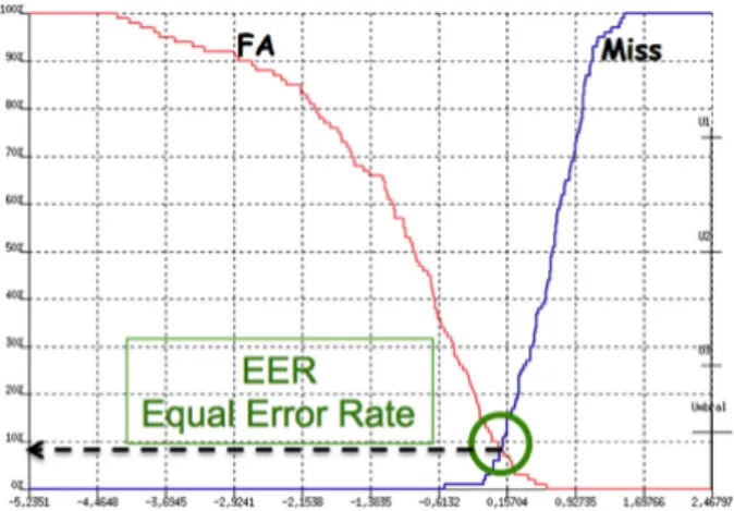
In Figure 2, both false acceptance and miss detection errors are shown as a function of a sweeping threshold. The error rate obtained where both false acceptance and miss detection curves cross each other is known as the Equal Error Rate (EER), and it is commonly used as a single number characterizing system performance: the lower the EER the better the separation between both target and non-target score distributions.

Figure 2:Percentage (%) of alse alarms and miss detections as function of a sweeping threshold (x-axis), and Equal Error Rate

(EER).

However, multiple error curves with different shapes, possibly overlapping and crossing each other, can result in the same EER, making it difﬁcult to compare different systems. An alternative single curve representing all possible operating points of the system is usually pre- ferred, as shown in Figure 3, known as Receiver Oper- ating Characteristic (ROC) curve, where all the pairs of errors (false alarm, miss) for a sweeping threshold are represented as points in the false acceptance versus missed detection plane, and connected with a single line. The advantage of a ROC plot is that it represents all the

(5)

operating points of a system in a single curve, allowing easy comparison of systems (the closer to the origin of coordinates, the better). Moreover, the commonly used EER point is easily extracted where the ROC curve crosses the diagonal straight line where false acceptance errors equal the missed detection errors.

Figure 3:Receiver Operating Characteristic (ROC) curve sum- marizing false alarm and miss detection curves. EER (%) is easily obtained where the ROC curve crosses de FA=miss diagonal.

However, when different systems (or the same system in different evaluation conditions) with low EER are represented, the graphical resolution is very low as all the useful information is concentrated in the lower corner close to the origin of coordinates. The Detection Error Trade-off (DET) plot is suggested to overcome this problem, modifying the axis in order for Gaussian distribution of scores to result in straight lines in the DET plot, allowing for easy comparison and detailed analysis of different possible operation points of the system, as shown in Figure 4.

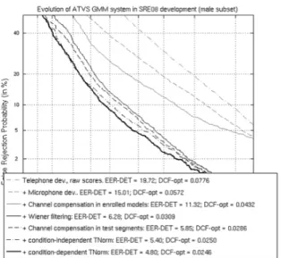
Figure 4:Sample DET curves from the development phase of ATVS-UAM systems for SRE 2008. The telephone-based SRE 2006 GMM-UBM system is progressively adapted to the cross-

channel mic and tel condition in 2008.

3.2. Cost function

In Section 3.1 we have shown how to evaluate the goodness of the discrimination abilities of a system. However, equally interesting is to know about the goodness of the decisions (acceptance/rejections) of a system for a given application of interest. Applica- tions are characterized by two factors: the relative cost of a false alarm versus a miss detection, and the

a prioriprobability of observing target and non-target speakers. We can illustrate those two factors with opposite applications where we could use exactly the same speaker recognition system with differing detection thresholds. Firstly, imagine a non-critical user- friendly application, of little interest to attackers or impostors. Here, the a priori probability of being a true user is high (P_target≥ P_non-target), and system designer will look not to disturb them in excess, so Cmiss≥ CFA. If in contrast we have a high-security application, costs will verify CFA>> Cmiss. If we look for a given speaker in big data repositories, where the probability of finding the target speaker is very low, a priori probabilities will verify P_target<< P_non-target.

For a given discrimination capability, depending on the selected threshold the system can observe different probabilities of false alarm, PFA|non-target, and miss detection, P_miss|target. NIST have used for their Speaker Recog- nition Evaluations (SRE) a composite cost function in order to rank participant systems where, given the application-dependent parameters Cmiss, CFAand Ptarget(Pnon-target = 1 - P_target), and the system-dependent probabilities PFA|non-target and Pmiss|target, an objective cost function CDET can be computed:

[1] C_DET= C_miss · P_target · P_miss|target+ C_FA· P_non-target · PFA|non-target

It is important to note that CDETcan only be computed

a posteriorionce the correct labels are known, that is, after the evaluation session. This means that participant systems have to select in advance their decision threshold for the given application parameters, and once results are submitted, NIST tells participants their actual C_DET. But once the solution labels are known, it is also possible to compute which was the optimal threshold of the system for the given discrimination, which provides the minC_DETvalue. Systems with close values of C_DETand minCDETare well calibrated, while the bigger the difference, the bigger the calibration loss. We have to highlight that it is possible to have a very good discriminant system with a very bad performance at the evaluation because of a bad threshold selection. Therefore, threshold selection is maybe the most critical part of a NIST submission, as it has the biggest direct impact in the system’s associated cost.

However, submitting system scores in the form of calibrated likelihood ratios is strongly recommended. Doing so, there is no longer a need to set any detection threshold, as the detection threshold is directly obtained

(6)

from these application-parameters. The system will be then application independent, meaning it is valid for any given application (access-control, customer-oriented, forensic…) whatever the application-parameters (a priori probabilities of targets, and relative costs) (Brümmer, 2010;; Ramos, Gonzalez-Rodriguez, Zadora, & Aitken, 2013;; van Leeuwen & Brümmer, 2007). Additionally, this is extremely useful for applications such as forensics (Gonzalez-Rodriguez et al., 2007;; Rose, 2002) where priors and costs are unknown (case- and legal-system dependent) and the reported likelihood ratios must be valid for whatever priors and costs are given (if any). 4. THE EARLY NIST SRES (1996-2001):

ACOUSTIC-SPECTRAL SHORT-TERM SYSTEMS

Text-independent speaker recognition technology in the 90’s was dominated by the GMM-UBM approach (Reynolds, Quatieri, & Dunn, 2000). Under the assump- tion of frame independence, the short-term cepstral vectors representing the spectral content every (typically) 10 milliseconds are modeled through a generative model consisting in a weighted combination of multi- variate Gaussian mixtures. This Gaussian Mixture Model (GMM) is expected to represent the observed features from the speaker in a cumulative way, which are taken as observations from this underlying model. GMMs, with high number of gaussians, were originally trained as maximum likelihood estimates from the training data, producing a large dependence for optimal systems on the duration of the available training material, as the number of free parameters to be estimated from data grows with higher number of gaussians. It was soon observed that a GMM representing all the available feature vectors from a given reference population, known as Universal Background Model (UBM) was very useful to normalize the score from the GMM, adding substantial robustness to duration variability. Finally, Maximum a Posteriori (MAP) adaptation of the speaker GMM from the UBM, where only the means of the gaussians are adapted to the speaker data, became the state-of-the-art at the time, being also the reference system to be compared with for almost two decades.

But those GMM-UBMs were severely affected by different sources of variability, such as available durations for training and test, type of telephone handset (carbon vs. electret), or land-line versus cellular phone calls. Those early evaluations were then designed to explore the limits and assess the performance of those systems in a variety of conditions to be sketched here. 4.1. Task deﬁnitions, corpora and evaluation

conditions

Different tasks were explored in those early evaluations, butone-speaker detection, the task of determining

if a given speaker is actually speaking in a given conversation side, has always been the main subject of evaluation. For every trial, participants are required to submit both a score indicating the conﬁdence in being the same speakers, which allows NIST computing DET plots, and an actual decision value (true/false), allowing CDETand minC_DET values to be computed per participant. Male and female data is included, but no cross-trials are performed to avoid over-optimistic error rates.

Figure 5:Faunagram, or speaker-dependent performance plot, showing non-target (red) and target (blue) scores per speaker. Models are vertically sorted as a function of the speaker-depen-

dent EER threshold.

Conversations were extracted from the English-spo- kenSwitchboardcorpus, a spontaneous conversational speech corpus consistent of thousands of telephone conversations from hundreds of speakers, each conversation typically running through 5 minutes. In 2000 and 2001, the Spanish-spoken spontaneous but not conver- sationalAhumadadatabase (Ortega-Garcia, Gonzalez- Rodriguez, & Marrero-Aguiar, 2000) was explored with similar same-language (in train and test) protocols. Different releases of Switchboard were produced through the years (Cieri, Miller, & Walker, 2003), including extensive landline (local- and long-distance) and cellular (GSM and CDMA) phone data. Different telephone numbers and types of telephone handsets were used by the speakers and explored in the evaluations, showing the degradation on performance in mismatched conditions if not properly addressed. Systems were tested with one- or two-session training, signiﬁcantly reducing the sensitivity to session mismatch by including explicit session variability in the model with the use of multiple session training. The effect of the length of the test was also explored, showing very limited beneﬁt from same-session audio segments longer than 30-60 seconds, but strong degradation for shorter durations. However, with just 3 seconds of speech, systems were still providing very useful information (e.g., degradations

(7)

from 6% of EER with 30 seconds of test speech, to 15% of EER with just 3 seconds of speech). To give an idea of the complexity of each task, the cellular evaluation of 2001 involved 190 speakers and 2200 test speech segments, resulting in thousands of cross-speaker trials. For interesting details on the early evaluation campaigns and summary of systems and results in different conditions, readers can refer to (Doddington, Przybocki, Martin, & Reynolds, 2000).

Different additional tasks were deeply explored be- sides one-speaker detection.Two-speaker detectionis essentially the same as one-speaker, but the test conversation includes both speakers (summed channels) in the conversation. A two-speaker mode for model training was also explored, where a target speaker was present in three different summed channel conversations with three different speakers. The task ofspeaker segmenta- tion(later calleddiarization) has also been largely explored, which is the task of determining the time inter- vals during which unknown speakers are actually speaking in different datasets from telephone conversational speech, broadcast news and recordings of multispeaker meetings.Speaker trackingwas also explored from 1999 to 2001, being the task of determining the time instants where a known speaker was actually speaking in a multispeaker conversation.Unsupervised adaptation, where trials are presented sequentially and accepted ones can be used to further improve the model for future trials, was also explored from 2004 to 2006. Finally, in 2010 and 2012, aHuman Assisted Speaker Recognition (HASR) task was proposed, where any combinations of machines, naive listeners or human experts were allowed in order to perform speaker detection over a manual selection of “especially difﬁcult” trials from the core condition (Greenberg et al., 2011). 4.2. Challenges for GMM-UBM systems

In order to tackle all the sources of variability described above, short-term spectral systems had to be improved significantly. Cross-condition trials with handset, telephone number, and landline/mobile variability stressed the need for robust “channel-independent” features. Different channels show different long-term frequency responses, severely influencing with a cepstral additive component throughout the utterance to the short-term spectral estimates of the speaker. Cepstral mean (and variance) substraction (Furui, 1981) proved useful in reducing channel effects. RASTA band-pass filters (Hermansky & Morgan, 1994), which additionally filter out frequency modulations not expected from speech, also helped to improve system performance. But channels are not strictly time-invariant, and time- dependent feature warping (Pelecanos & Sridharan, 2001) in sliding windows of 3 seconds significantly contributed to the robustness of the systems, making CMN-RASTA-Warping a by-the-time standard front end.

However, pooling together the scores from all target and non-target trials in order to compute a single DET plot, EER value or C_DET for a given system arose the problem of score misalignment. When we talked before about the target and non-target score distributions, we would like to observe similar distributions for all speakers (assuming gaussianity this means similar means and variances). However, it is well known that thefauna

of speakers is varied (Doddington, Liggett, Martin, Przybocki, & Reynolds, 1998). While most speakers in a experiment behave similarly (sheep), some of the speakers are difficult to be correctly recognized (goats, target trials with low scores), some of the speakers are easy to be imposted (lambs, or speaker models giving high scores in non-target trials), and some of the speakers are successful imposting other speakers (wolves, speakers in non-target trials with high scores when ac- cessing other speaker models). This behavior is illustrat- ed in figure 5 (we called that plot afaunagram), where each horizontal line represents actual non-target and target scores for a given model, and models are vertically sorted as a function of their speaker-dependent EER threshold, clearly showing that almost all speakers show different means and variances of both target and non- target distributions. Even though the discrimination per speaker was reasonable (for instance, a low average of the EERs per speaker), for any single global threshold we select, the global EER will be significantly lower, as some speakers will be favored but some others will be strongly penalized.

In order to have a “common” non-target distribution for all speakers, scores are usually Z-normalized. This technique, known asZ-norm, estimates the distribution (mean and variance) of non-target scores of a given model using an external cohort of impostor trials, usually formed by other utterances from speakers different from the target, ideally in conditions similar to those of the testing environment. Then, all trial scores from this model are normalized to a zero mean unity variance Gaussian simply subtracting its speaker-dependent mean and dividing by its standard deviation. Once all speakers share a common impostor distribution, a single global threshold can be set giving a global EER close to the average of the EERs per speaker.

As cohort speakers for Z-norm are selected from the available data in the development phase, there is always some mismatch between their scores and the actual non- target distribution in the test phase, so some residual misalignment is always present. Moreover, different channels or handsets produce different non-target distributions (one per channel/handset). This is whyH-norm

(Handset normalization) was proposed, which is a dou- ble version of Z-norm, one per handset (carbon/button). During a test-time a decision about the estimated handset is needed in order to use the proper handset parameters for normalization. This is done simply scoring the input utterance against two UBMs, one per handset, and se- lecting the one giving the highest score (Reynolds et al., 2000). However, for multiple cross channel conditions,

(8)

the large number of combined “channel” models would make unlikely for them to be properly identiﬁed, so more sophisticated approaches to channel compensation are needed, as will be shown in section 6.2.

A second approach to score normalization known as

T-norm became extremely popular (Auckenthaler, Carey, & Lloyd-Thomas, 2000). In this case, the non-target score distribution is estimated with the actual test speech against a cohort of (external) speaker models. This normalization is extremely efficient as it takes also into account the length of the input speech, acting also as a kind of test-duration normalization. Moreover, T-norm usually had the effect of a counter-clock-wise tilt of the DET curve. Then, as the usual application parameters in NIST evaluations for one-speaker detection resulted in upper-left (in the DET plot) desired operation points, T-norm not only benefited the discrimination but had an enormous benefit for the calibration of the system, allowing for detection thresholds resulting in much lower CDET values. The joint use in cascade of Z- and T- norm, known as ZT-norm has become a standard score normalization technique that systems have success- fully used for more than a decade.

5. GOING HIGHER (2002-2005): SUPRA-SEGMENTAL SYSTEMS

In the inﬂuential and pioneering work presented in (Doddington, 2001), word bi-grams were computed just from the word transcriptions provided by an ASR giving excellent speaker recognition results. Moreover, signif- icant gains were reported from more and more training and testing data, as opposed to short-term spectral systems whose performance saturates beyond 30-60 seconds of test speech and two sessions for training. This success resulted in an explosion of approaches taking advantage of non-cepstral information. Using different speaker information extraction techniques, as shown in section 2.2, participants developed different nature systems with a common objective for exceptionally demanding new tasks and conditions as will be shown in Section 5.1. 5.1. Task deﬁnitions, corpora and evaluation

conditions

While early evaluations focused on telephone channel (landline versus cellular), handset (carbon vs. electret) and duration effects, NIST evaluations since 2001 included new data types and conditions, and since 2004 through the use of the new Mixer corpus, which broad- ened the scope of evaluation of speaker recognition systems, the evaluation data allowed for large multisession training, multi-microphone recording and multi- lingual speakers (bilingual speakers of English and a second language).

The extended data task allowed for multi-session training of speakers, providing up to 16 conversations

to train every speaker. Training conditions were explored with speech lengths of 10 seconds (from one conversation side), 1 full conversation side (average 2.5 minutes of speech), 3 sides (average 7.5 minutes of speech), 8 sides (20 minutes of speech) and 16 sides (40 minutes of speech). Those conditions provided enough data for non-segmental speaker recognizers requiring longer speech segments to fully exploit the different prosodic, ASR-conditioned and idiolectal high level systems. Different test segment lengths have also been explored, namely 10 seconds, 30 seconds, 1 side (average 150 seconds) and 1 summed-channel conversation (5 minutes from two speakers). Short-term cepstral systems had then the opportunity to focus on the demanding 10s-10s condition or the regular 1side-30 seconds, while high- level systems focused in the much bigger 8- or 16-sides training tasks.

Moreover, multichannel microphone datawas obtained from hundreds of speakers who made some of their calls from one of three special on-site recording rooms where simultaneous recording of the phone conversations were obtained from eight different microphones:

• Ear-bud/lapel mike • Mini-boom mike • Courtroom mike • Conference room mike • Distant mike

• Near-ﬁeld mike • PC stand mike • Micro-cassette mike

For instance, in tests performed with telephone-only data training, cross-microphone tests trials showed degradation from 2% EER for telephone test speech, to EER values from 4% to 8% depending on the microphone type, doubling or quadrupling the error rates. This multi-microphone data allowed for extensive testing of cross-channel conditions, converting the “discrete” previous channel variability (e.g., two handsets, or two types of telephone connections, etc.) in a “continuous” source of variation due to the large number of combinations of microphones, handsets, telephone channels and train/test durations, motivating a new ”continuous” approach to session and channel variability, as will be shown in 5.3 and will explode as the core technique to state-of-the-art speaker recognition in section 6.2.

TheMixer corpora, in order to explore language effects on performance, have included hundreds of ﬂuent bilingual speakers in English and a second language, namely (numbers are given for SRE 2004):

• Arabic (52 speakers) • Mandarin (46 speakers) • Russian (48 speakers) • Spanish (79 speakers) • English only (85 speakers)

Those 310 target speakers in SRE 2004 allowed checking that for matched language trials results were

(9)

mostly independent of the chosen language. However, for mismatched trials (the speaker uses different languages for train and test), a signiﬁcant but not dramatic drop of performance was observed (e.g., from 3% EER for matched language trials to 8% EER for mismatched language trials).

In order to give an idea of the computational complexity of those evaluations, NIST departed from some thousands of trials in the early evaluations to about 26,000 trials (comparisons) involving over 400 speaker models in the SRE 2004 1side-1side task, or 80,000 trials from 1,900 speaker models (same speakers in different training conditions) for the SRE 2004 multisession (16- , 8-, 3- and 1-side) training trials.

5.2. Higher-level systems

In those years two different approaches were developed to further advance the current performance of speaker recognition systems in the presence of such challenging channel and language variability. The first approach, described in this section, took advantage of the much larger amounts of data and explicit session variability included for training in the extended data tasks with up to 16 full conversation sides, which were used for training prosodic and phone- and lexical-sequence based speaker models. The second approach, described in Section 5.3, faced channel and session variability through new cepstral-based ways of representing an utterance in a high-dimensional space, allowing for much better results in classical 1side-1side and shorter tasks as 1side-10sec or 10sec- 10sec.

The different high-level approaches that were adopted can be exempliﬁed from those reported in the 6-week summer workshop in 2002 at John Hopkins University (Reynolds et al., 2003). The 2001 NIST extended data was the reference task which used the entire Switchboard I conversational telephone speech database, with models trained up to 16 full conversation sides (about 40 minutes of speech), having close to 500 speakers and 4100 models (different models for different amounts of training data) and 57,000 test trials involved. To summarize, several families of systems were developed (results are provided for the 8-conversation training condition):

• Acoustic: a 2048 mixture cepstral-based GMM- UBM built from Switchboard II external data was used as reference system, providing an EER of only 0.7%.

• Prosodic: pitch and energy distributions and dynamics, through the joint slope modeling of pitch and energy contours gave an EER of 9.2%, which dropped to 5.2% when adding phone context to duration and contour dynamics. Additionally, a different system using 11 duration-derived statistics and 8 pitch related statistics obtained an EER of 8.1%.

• Phone-sequence: the idea of those systems is to exploit the information provided by simultaneous multiple open-loop phone recognizers in different languages. An open-loop recognizer is basically a speech recognition system without any language modeling, providing just the most likely sequence of phones without any linguistic constraint. Current open-loop phone recognizers have very high phone error rates (usually bigger than 30-40%), but they are expected to produce “speaker-dependent” transcriptions, as they are expected to err consistent- ly for a given speaker. The combined used of phone n-grams from 5 different speech recognizers in 5 different languages (PPRLM) obtained an EER of 4.8% in the 8-conversation reference condition, while binary trees with a 3 token history (equivalent to 4-grams) obtained a 3.3% EER in the same task. Another system exploited the cross-stream information from the multiple phone streams, obtaining a 4.0% EER, which fused with the PPRLM was reduced to 3.6%.

• Pronunciation modeling: comparing constrained word-level ASR phone streams (the “true” phone sequence) with error-prone open-loop phone streams, speaker-dependent pronunciations were learned, obtaining an EER of 2.3%.

• Lexicalfeatures: n-gram idiolect systems as those described above in Doddington (2001) were tested, providing an EER of 11% from the best-available ASR word transcriptions.

• Conversationalfeatures: feature vectors were derived from turn-taking patterns and conversational style based information from pitch and durations, then converted into n-grams which obtained an EER of 15.2%.

Fusion of classiﬁers is strongly beneﬁted from minimum correlation between systems to be fused. High- level systems produced excellent error rates with extremely different features and models from those in short-term cepstral-based GMM-UBM, which represented by the time the state-of-the-art of speaker recognition. When the non-cepstral systems were fused in the 8- conversation train task, the fused EER was exactly the same (0.7%) of the cepstral GMM-UBM system. Moreover, when all high-level and acoustic systems were combined, the reported EER was only 0.2%, a 71% relative reduction from incorporating high-level knowledge to a reference cepstral-based system. A similar combination of cepstral and high-level systems in an actual submission to NIST SRE 2004 is described in Kajarekar (2005).

5.3. High-dimensionality spectral systems

The GMM-UBM is a generative modeling approach, where the underlying model (the GMM) is supposed to be “generating” the observed features. In the late 90’s, a new discriminative pattern recognition technique

(10)

known asSupport Vector Machine(SVM) (Schölkopf & Smola, 2002;; Vapnik, 1995) showed to be extremely efﬁcient discriminating objects (points) in very high dimensional feature spaces. SVMs are easily trained, the SVM speaker model being the hyperplane separating the target training speaker utterances (one or several points) from all non-target speaker utterances (lots of points). The score from an unknown utterance with respect to a given SVM model is obtained as a signed distance to the separating hyperplane. But in order to use SVM, low-dimensional feature vectors (as cepstral vectors or n-gram probabilities) must be transformed into separable high-dimensional vectors, which is done bykernels(or transformations).

Different kernel-tricks were proposed to transform a speech utterance, represented usually as a sequence of observed feature vectors, into a very high dimensional space representation. While GLDS (Campbell, Camp- bell, Reynolds, Singer, & Torres-Carrasquillo, 2006a) or MLLR (Stolcke, Kajarekar, Ferrer, & Shrinberg, 2007) supervectors were also successful, we highlight here the Gaussian (or GMM) supervector (GSV) concept (Campbell, Sturim, & Reynolds, 2006b), being a natural extension of the well-known GMM-UBM framework. A GMM of M Gaussian mixtures in P feature dimensional space (cepstral vectors of dimension P) is composed of M weights, MxP means and MxP variances (assuming diagonal covariance matrices). But as MAP adaptation of the GMM from the UBM is usually performed just over the means (weights and covariance matrices are shared across all speakers), one UBM-adapted speaker GMM differs from another GMM of a different speaker just in their means. A supervector is then just the stacked pile of all GMM means (after variance normalization), a vector of MxP values, or a single point in an MxP dimensional space. As typical values of M are 1024 or 2048, and P takes values from 20 to 60, speech utterances will then be represented by vectors of size 20k to 120k, in other words, by points in a 20k-120k dimensional space.

Once utterances are reduced to points in a high-dimensional space, the problem of session variability

(between-session differences in the speaker information) becomes variability between points, with some dimensions (directions) more severely affected than others. The problem of session variability compensation can be then addressed estimating the principal directions of channel variability in the development phase, and later canceling them out in the test phase, a process known asNuissance Attribute Projection(NAP) (Solomonoff, Campbell, & Boardman, 2005). If we compute for every speaker in the development set the mean supervector (one per speaker), and every utterance is normalized subtracting its mean speaker vector, the resulting data set (known aswithin-scattermatrix) with all normalized utterances contains only session variability and no speaker information. Then, an eigenvector analysis (PCA, Principal Components Analysis) of this within- scatter matrix will provide the desired principal direc-

tions of channel variability, known aseigenchannels. In the test phase, we can easily project every unknown supervector into those channel dimensions, and subtract the resulting supervector (which should contain the session variability components) from the original one. In order to get an idea of the signiﬁcant improvements obtained with GSV-SVM and NAP facing channel variability, readers are referred to Campbell et al. (2006b).

6. BIG DATA EVALUATIONS (2006-2012): SESSION VARIABILITY COMPENSATION

Since 2006, NIST SREs became biannual, and have introduced signiﬁcant changes evaluation after evaluation, as shown below in 6.1, additionally introducing massive amounts of new data in every new evaluation. But the biggest difference, as highlighted in Brümmer et al. (2007), is that especially from SRE 2006, “systems no longer train individual speaker models from some minutes of speech, but whole systems are trained on hundreds of hours of speech in whole NIST SRE databases” (p. 2082), transforming the conceptually simple speaker detection task, classically seen as that of comparing two utterances to determine if they come or not from the same speaker, into a seriousbig data

task where systems are designed to jointly optimize the detection of thousands of speakers in hundreds of thousands of comparisons, where the speech segments in the comparisons are tens of thousands of utterances of varied and mixed channel, speaking style, duration and noise characteristics.

6.1. Task deﬁnitions, corpora and evaluation conditions

The last four evaluations in the NIST SRE series have introduced major changes from evaluation to evaluation that can be summarized as follows:

• SRE 2006: the eightalternate microphonesfrom Mixer 3, as shown in section 5.1, were fully exploited. Additionally, analternative cost function, Cllr, is included as optional but soon became widely used being usually the objective function for cost minimization in fusion of systems. The number of trials in the required (1side-1side) condition was about 54,000.

• SRE 2008: up to 2006, evaluations dealt with spontaneous conversational speech obtained in telephone conversations between remote speakers. The Phonecall conversational speech database, known as Mixer 3, was used for SRE 2008. Addi- tionally to regular telephone recordings (phonecall- phn), conversational telephone speech recorded over a microphone channel (phonecall-mic) is also included in the test conditions. But for SRE 2008, a new type of speech was recorded in an on-site

(11)

interview scenario, resulting in the Mixer 5 Inter- view speech database. It is also conversational speech but of a totally different nature, and it is recorded via multiple simultaneous microphones (interview-mic). In the required condition (known as short2-short3, similar to a multichannel1side- 1side), 1,788 phonecall and 1,475 interview speaker models were involved for a total of almost 100,000 trials (60,000 male and 40,000 female). • SRE 2010: four new signiﬁcant changes were in-

troduced in 2010. Firstly, all speech in the evaluation was English (both native and non-native). Second, some of the conversational telephone speech data has been collected in a manner to produce particularly high or particularly lowvocal ef- fort. Third, the interview segments in the required condition were ofvarying duration, ranging from three to ﬁfteen minutes. And ﬁnally, the most rad- ical change, a new performance measure

(new_CDET), intended for systems to obtain good calibration at extremely low false alarm rates, was deﬁned from a new set of parameter values. While C_DETalways used C_miss=10, C_FA=1 and P_target=0.01, the new_CDET parameters are Cmiss=1, CFA=1 and P_target=0.001, increasing in a factor of 100 the relative weight of false alarms to missed detections. In order to have statistically signiﬁcant error rates for very low false alarm rates, the required (core) condition included close to 6,000 speaker models, 25,000 test speech segments and 750,000 trials. • SRE 2012: in NIST’s own wording, “SRE12 task

conditions represent a signiﬁcant departure from previous NIST SRE’s (NIST 2012, p. 1)”. In all previous evaluations, participants were told what speech segments should be used to build a given speaker model. However, in 2012, all the speech from previous evaluations with known identities was made available to build the speaker models, resulting in availability of large (and variable) number of segments from thephone-tel,phone-mic

andint-micconditions, systems being free to build their models using whatever combination of previous ﬁles from every speaker. Moreover, additive and environmental noises were included, variable test durations (300, 100 and 30 seconds) considered, knowledge of all targets was allowed in computing each trial detection score, tests were performed with both known and unknown impostors, and for the ﬁrst time in a long time ASR word transcripts were not provided. Finally, the cost measure was changed again, averaging the 2010 operating point (optimized for very low false alarm rates) with a new one with a greater target prior (pushing the optimal threshold back, closer to its “classical” position), intending for systems to show greater stability of the cost measure and good score calibration over a wider range of log-likelihoods. For this evaluation, close to 2,250 target speakers and 100,000 test segments were involved, for a total

in the required (core) condition of 1,381,603 trials. For those involved in the (optional) extended trials task, the number of trials was 67,000,000. Factor analysis and i-vectors

Even though one site continued to submit successful high- and low-level combined systems in those big data evaluations (Ferrer et al., 2013;; Kajarekar et al., 2009;; Scheffer et al., 2011), there was a consensus in turning back to cepstral-only systems. The computational complexity of higher-level systems and the relative improvements obtained in limited training data conditions helped the community to move towards a scientifically complex but very rewarding approach because of the performance and computational efficiency of new high-dimensional spectral systems as JFA-compensated GMM-UBM, and later, i-vector front-end extraction and PLDA based classification.

Different supervectors from different recordings of the same speaker show severe variability due tointers- ession variability, accounting for channel and speaker speciﬁc variability. In order for a test supervector to be close to the target speaker one, intersession variability, usually called just “channel” variability, must be compensated. Joint Factor Analysis (JFA) (Kenny, 2005) models channel variability explicitly, taking the variability of a supervector as a linear combination of the speaker and channel components. In order to know and compensate the channel “offset” in a test utterance, the main directions of channel and speaker variability in the high-dimensional space have to be found in advance from large development datasets. The eigenchannels matrix can be initialized through PCA of the within- scatter matrix as shown in 5.3, and theeigenspeakers

(also calledeigenvoices) one in a similar way from the

between-scattermatrix, that is, a data structure with one column per speaker, where every column is the speaker mean vector (mean of the different session-dependent speaker supervectors) minus the global mean of all speaker means. After this PCA initialization of both matrices, they are improved through several Expectation- Maximization (EM) iterations over the whole development dataset. Once the eigenchannel and eigenspeaker matrices are estimated, the channel and speaker factors in a test utterance are jointly estimated as point estimates as in classic relevance MAP. Then the channel factor can be discarded, and the “clean” speaker supervector, estimated as the offset from the UBM supervector in an “amount” given by the speaker factor in the eigenspeaker directions, can be used for recognition with a synthesized “clean” GMM model or a SVM with “clean” supervectors. JFA-based approaches, in several of the numerous ﬂavours of this technology, have obtained excellent results in the 2006 to 2010 NIST SREs.

However, it was shown that the channel factors, which are to be discarded from the model, still contain information from the speaker. Then, instead of assuming

(12)

two different variability subspaces (speaker and channel), in (Dehak, Kenny, Dehak, Dumouchel, & Ouellet, 2011) a single subspace is considered, called Total (T) Variability subspace, which contains both speaker information and channel variability. In this case, the T low- rank matrix is obtained in a similar way to the eigen- speakers matrix but all the utterances for each speaker are included (as if each of them came from different speakers). Once the T matrix is available, an UBM is used to collect Baum-Welch first-order statistics from the utterance. The high-dimensional supervector (dimensions ranging from 20,000 to 150,000), which is built stacking together those first order statistics for each mixture component, is then projected into a low dimensional fixed-length representation known as the i-vector in the subspace defined by T, being estimated as a MAP point-estimate of a posterior distribution.

As both target (train) and test utterances are now represented by ﬁxed-lentgh i-vectors (typically from 200 to 600 dimensions), it can be seen as a new “global” feature extractor, which captures all relevant speaker and channel variability in a given utterance into a low- dimensional vector. Target and test i-vectors can be directly compared through cosine scoring, a measure of the angle between i-vectors, which produce recognition results similar to those with JFA. But as they still contain both speaker and channel information, factor analysis can also be applied in the total variability subspace to better separate low dimensional contributions of channel and speaker information. Probabilistic Linear Discrimi- nant Analysis (PLDA) (Prince & Elder, 2007) models the underlying distribution of the speaker and channel components of the i-vectors in a generative framework where Factor Analysis is applied to describe the i-vector generation process. In this PLDA framework, a likelihood ratio score of the same speaker hypothesis versus the different speaker hypothesis can be efﬁciently computed, as a closed form solution exists. Further, in order to reduce the non-Gaussian behavior of speaker and channel effects in the i-vector representation, i- vector length normalization (Garcia-Romero, & Espy- Wilson, 2011) is proposed allowing the use of probabilistic models with Gaussian assumptions as PLDA instead of complex Heavy Tailed representations.

I-vector extraction, PLDA modeling and scoring, and i-vector length normalization have become by the time of writing this paper the current state-of-the-art in text-independent speaker recognition, and the basis of successful submissions to NIST SRE 2012. Multiple generative and discriminative variants, optimizations and combinations of the above ideas exist based in the same underlying principles. As a result, joint submissions to NIST SREs of multiple systems from multiple sites into a single fused system have become usual, and a must if an individual system wants to be in the horse- race photo-ﬁnish of best submissions (Saeidi et al., 2013).

However, recent success of Deep Neural Networks in different areas of speech processing (Hinton et al.,

2012;; Lopez-Moreno et al., 2014) promise for the near future exciting developments in speaker recognition, as those advanced in Vasilakakis, Cumani, and Laface (2013), and Variani, Lei, McDermott, Lopez-Moreno, and Gonzalez-Dominguez (2014).

7. DEMYSTIFYING SREs: THE 2014 NIST I-VECTOR CHALLENGE

As shown in the above sections, NIST Speaker Recognition Evaluations have always demanded from participants a very complex machinery of signal processing, pattern recognition, data engineering and computational resources. A newcomer to the evaluations receives hundreds of hours of speech data from previous evaluations as development data, with varied data structures and different segments and speaker identity labeling formats in a mixture of conditions (channels, speaking style, durations…). Even if having available and properly working all the software components to build a system, the human and computational resources to be spent for voice activity detection, feature extraction, universal background modeling, estimation of variability subspaces, etc., with the proper separation of conditions and tasks, is a major access obstacle that inhibits many potential participants from enrolling in the evaluations. In order to eliminate this barrier and promote participation from pattern recognition scientists working in different areas, a simplified exercise has been proposed in 2014 consisting in the classification and recognition of a large amount of properly-extracted but unlabeled i-vectors (speaker identifiers are not provided). More- over, a good i-vector cosine-scoring reference system is provided, with all the necessary scripts to work with the evaluation data and submit results of the evaluation. Additionally, NIST has made available an on-line cost scoring system (over 40% of the test data) that provides participants in real-time a good estimate of the goodness of every new algorithm or tuning factor they have tested. And finally, all participant-best (minimum) costs and associated submitting site names are known every time a participant submits a new system, promoting a horse- race competition where all participants see each other progress.

By the time of writing this paper, the participation level in the 2014 i-vector challenge is a major success, and the reported cost improvements over the reference system promise exciting news in the form of new or optimized algorithms to be presented in the NIST challenge workshop to be held during the Odyssey Speaker and Language Recognition conference in June 2014. 8. DISCUSSION AND CONCLUSION

The NIST series of Speaker Recognition Evaluations is a good example of how to foster tremendous progress in a specially challenging problem from a simultaneously

(13)

competitive and cooperative scientiﬁc community. Nevertheless, linking the progress in speaker recognition to participation in the NIST cycle of evaluations is not free of inconveniences.

First of all, participants cross-benefit from the other participants publications and previous submissions, resulting in a pseudo-normalization of procedures and system components, with plenty of submissions differing in very slight details. Moreover, high-risk innovation is indirectly penalized as new alternative approaches are unable to reach or help existing state-of-the-art systems, the task being so complex and mature that participants tend to bet on winning horses. And finally, being a competitive evaluation according to a given cost function with a final rank of participants in every task, and given the benefits of fusing multiple classifiers in a complex task like this, participants tend to group themselves in large consortia, both to minimize risks and opt to better ranking, submitting valid but unrealistic fusions of multiple (even tens of) systems.

Speaker recognition systems have shown extremely good performance and computational efficiency when lots of development data, in conditions close to the evaluation (application) data, are available. However, the current biggest challenge to speaker recognition is how to adapt this well-proven technology in known domains to new applicationswhenlittle(comparedtothehundredsofhours of data in NIST SREs) or no development data is available in new unknown conditions (language, channels, speaking style, audio quality, etc.). Related challenging issues are those of calibration in highly mismatched environments, the production of reliable automatic recognition results from descriptive speech features (pronunciation patterns, voicequality,prosodicfeatures…)correlatingwithlinguists and phoneticians observations, or measuring the goodness of the system decisions in individual comparisons, that is, how reliable is one system in the unknown comparison at hand, not globally in thousands of known comparisons.

However, in spite of the inconveniences and out-of- domain limitations, it is extremely beneﬁcial for system developers to be involved in the evaluations. There is a huge gap between developing a new system in the labo- ratory or trying a new pattern recognition algorithm and being able to obtain good results in the demanding conditions of the NIST evaluations. And only when tested in really challenging environments, speaker recognition systems will be a step closer to being usable in daily applications.

REFERENCES

Adami, A. G., Mihaescu, R., Reynolds, D. A., & Godfrey, J. J. (2003). Modeling prosodic dynamics for speaker recognition.

Proceedings of the 2003 IEEE International Conference on Acoustics, Speech, and Signal Processing (ICASSP ’03), 4, 788–91. http://dx.doi.org/10.1109/ICASSP.2003.1202761 Auckenthaler, R., Carey, M., & Lloyd-Thomas, H. (2000). Score

normalization for text-independent speaker veriﬁcation systems.

Digital Signal Processing, 10(1-3), 42–54. http://dx.doi.org/ 10.1006/dspr.1999.0360

Brümmer, N. (2010).Measuring, reﬁning and calibrating speaker and language information extracted from speech (doctoral dissertation). University of Stellenbosch, South Africa. Brümmer, N., Burget, L., Černocký, J., Glembek, O., Grézl, F.,

Karaﬁát, M., ... Strasheim, A. (2007). Fusion of heterogeneous speaker recognition systems in the STBU submission for the NIST speaker recognition evaluation 2006.IEEE Transactions on Audio, Speech, and Language Processing, 15(7), 2072–2084. http://dx.doi.org/10.1109/TASL.2007.902870

Campbell, W. M., Campbell, J. P., Reynolds, D. A., Singer, E., & Torres-Carrasquillo, P. A. (2006a). Support vector machines for speaker and language recognition.Computer Speech & Language, 20(2–3), 210–229. http://dx.doi.org/10.1016/j.csl.2005.06.003 Campbell, W. M., Sturim, D. E., & Reynolds, D. A. (2006b). Support

vector machines using GMM supervectors for speaker veriﬁcation.IEEE Signal Processing Letters,13(5), 308–311. http://dx.doi.org/10.1109/LSP.2006.870086

Cieri, C., Miller, D., & Walker, K. (2003). From switchboard to ﬁsher: Telephone collection protocols, their uses and yields.

Proceedings of the 8th European Conference on Speech Communication and Technology, EUROSPEECH 2003 – INTERSPEECH 2003, 1597–1600.

Davis, S., & Mermelstein, P. (1980). Comparison of parametric representations for monosyllabic word recognition in continuously spoken sentences.IEEE Transactions on Acoustics, Speech and Signal Processing, 28(4), 357–366. http://dx.doi.org/ 10.1109/TASSP.1980.1163420

Degottex, G., Kane, J., Drugman, T., Raitio, T., & Scherer, S. (2014, May).COVAREP - A collaborative voice analysis repository for speech technologies. To be presented at the 2014 IEEE International Conference on Acoustics, Speech and Signal Processing (ICASSP ’14), Florence, Italy.

Dehak, N., Kenny, P., Dehak, R., Dumouchel, P., & Ouellet, P. (2011). Front-end factor analysis for speaker veriﬁcation.IEEE Transactions on Audio, Speech, and Language Processing, 19(4), 788–798. http://dx.doi.org/10.1109/TASL.2010.2064307 Doddington, G. R. (2001). Speaker recognition based on idiolectal

differences between speakers.Proceedings of the 7th European Conference on Speech Communication and Technology, EUROSPEECH 2001 – INTERSPEECH 2001, 2521–2524. Doddington, G., Liggett, W., Martin, A., Przybocki, M., & Reynolds,

D. (1998). Sheep, goats, lambs and wolves: A statistical analysis of speaker performance in the NIST 1998 speaker recognition evaluation. Proceedings of the International Conference on Spoken Language, 1–5.

Doddington, G. R., Przybocki, M. A., Martin, A. F., & Reynolds, D. A. (2000). The NIST speaker recognition evaluation – Overview,

methodology, systems, results, perspective. Speech

Communication, 31(2–3), 225–254. http://dx.doi.org/10.1016/ S0167-6393(99)00080-1

Ferrer, L., McLaren, M., Scheffer, N., Lei, Y., Graciarena, M., & Mitra, V. (2013).A noise-robust system for NIST 2012 speaker recognition evaluation. Paper presented at the 14th INTERSPEECH Conference 2013, Lyon, France.

Furui, S. (1981). Cepstral analysis technique for automatic speaker veriﬁcation.IEEE Transactions on Acoustics, Speech, and Signal Processing, 29(2), 254–272. http://dx.doi.org/10.1109/ TASSP.1981.1163530

Garcia-Romero, D., & Espy-Wilson, C. Y. (2011). Analysis of i-vector length normalization in speaker recognition systems.

Proceedings of the 12th INTERSPEECH Conference 2011, 249–252.

Gonzalez-Rodriguez, J. (2011). Speaker recognition using temporal contours in linguistic units: The case of formant and formant-bandwidth trajectories. Proceedings of the 12th INTERSPEECH Conference 2011, 133–136.

Gonzalez-Rodriguez, J., Rose, P., Ramos, D., Toledano, D. T., &

Ortega-Garcia, J. (2007). Emulating DNA: Rigorous

quantiﬁcation of evidential weight in transparent and testable forensic speaker recognition. IEEE Transactions on Audio, Speech, and Language Processing, 15(7), 2104–2115. http:// dx.doi.org/10.1109/TASL.2007.902747

Evaluating automatic speaker recognition systems: an overview of the nist speaker recognition evaluations (1996-2014)

Evaluating Automatic Speaker Recognition systems: An overview

of the NIST Speaker Recognition Evaluations (1996-­2014)

of the NIST Speaker Recognition Evaluations (1996-2014)