Bayesian Estimation of the Weibull Parameters Based on Competing Risks Grouped Data

(1)

http://siba-ese.unisalento.it/index.php/ejasa/index e-ISSN: 2070-5948

DOI: 10.1285/i20705948v11n2p687

Bayesian estimation of the Weibull parameters based on competing risks grouped data

By Migdadi, Abu-Shawiesh, Almomani

Published: 14 October 2018

This work is copyrighted by Universit`a del Salento, and is licensed un-der aCreative Commons Attribuzione - Non commerciale - Non opere derivate 3.0 Italia License.

For more information see:

(2)

DOI: 10.1285/i20705948v11n2p687

Bayesian estimation of the Weibull

parameters based on competing risks

grouped data

Hatim Solayman Migdadi

∗

, Moustafa Omar Abu-Shawiesh, and

Mohammad H. Almomani

Department of Mathematics, The Hashemite University Zarqa, Jordan

Published: 14 October 2018

Based on the competing risks grouped data, Bayesian estimation approach is considered for the parameters of the Weibull distribution and the related specific hazard and survival functions. The estimation procedures are carried out under the square error loss (SELF) and linear exponential loss (LINEX) functions. High posterior (HPD) credible intervals for the specified param-eters are also obtained. The derived estimators are in explicit closed forms. Their properties and performance are illustrated through an application to real lifetime’s data and an extended simulation study. Overall results indi-cate that, the Bayesian estimators are dominated other estimators obtained by other methods and are recommended when continuous life testing is not available.

keywords: Weibull distribution, competing risks, grouped data, loss func-tion, HPD credible interval.

1 Introduction

In reliability and survival analysis subjects may be at risk of failure due to more than one cause, giving rise of what is known as competing risks analysis. Problems related with competing risks are extensively involved in reliability systems, medicine, engineering, economics and many other fields of studies that concerns with lifetime distribution of a

∗

Corresponding author: [email protected], mh [email protected]

c

Universit`a del Salento ISSN: 2070-5948

(3)

unit (individual, item, system) subject to several failure modes. Statistical inference for the parameters of the lifetime models using different censoring schemes with competing risks data are considered by many authors. Examples are Sarhan (2007); Alwasel (2009); Josmar and Jorge (2011); Shai and Wu (2016); Lai and Murthy (2003).

In many real practical settings, continuous monitoring the test units to have the required lifetimes data is not available, incorporate specific measurement errors, costly and needs hard efforts or not feasible in some situations. Therefore, it is more probable to inspect the units periodically for failure. Hence, the time line is initially divided into adjacent intervals to have the interval grouped data which consists of the numbers of failed or censored units in the given intervals. This type of data is frequently used in many areas of reliability and survival analysis. The Maximum likelihood estimation using a general interactive optimizer and grouped data is considered in Gove and Fairweather (1989). Pipper and Ritz (1989) have checked the grouped data for the Cox model. Aludaat et al. (2008) derived estimators of the Burr type X distribution parameters using the grouped data. Migdadi and Al-Batah (2014) investigated the Bayesian approach for the Weibull distribution based on the interval grouped data.

The Weibull distribution proposed initially by Weibull (1951), for describing the fa-tigue failures from the wear out materials. Recently, it has extensive applications in modeling a variety of real lifetimes data. Applications of the Weibull distribution are mainly addressed in Lowe and Lewis (1983); Yazhou et al. (1995); Lai et al. (2017); Rinne (2009); Mudholkar and Asubonteng (2010).

Consider the life testing experiment in which n units are put in the test for failure and are exposed to m possible risks. If the ith cause of failure comes from the Weibull model with common shape parameterγ and scale parametersλi, i= 1,2, . . . , m. Then the specific survival and hazard function for the ith mode are:

Si(t) =e−λitγ ₍₁₎

hi(t) =γλitγ−1, γ >0, λi>0, i= 1,2, . . . , m (2) If the lifetime of the unit comes from only one of the independent competing risks, then the overall survival and hazard functions are:

S(t) = Πm_i₌₁Si(t) =e−Σ m

1λitγ ₌_e−λtγ ₍₃₎

h(t) = Σm_i₌₁hi(t) =γ(Σim=1λi)tγ−1 =γλtγ−1 (4) whereλ= Σm_i₌₁λi.

Maximum likelihood and type moment Estimators of the Weibull parameters using competing risks grouped data are studied by David and Moeschberger (1978) and Lianfen and Jose (2003). Yanez et al. (2014) have studied the characteristics of two competing risks models with Weibull distributed risks. Iskandar and Gondokaryono (2016) con-sidered Bayesian analysis approach for the competing risk models in reliability systems

(4)

using a Weibull distribution. Dey et al. (2016) considered Bayesian analysis of the mod-ified Weibull distribution under progressively censored competing risk model. Bayesian inferences for the Weibull and other lifetimes models are also included in Prakash (2014), Pak and Chatrabgoun (2016), Tahir et al. (2017) and Pak and Rastogi (2018).

Statistical selection procedures are used in a variety of applications to select the best of a finite set of alternatives. “Best” is defined with respect to the (largest or smallest) mean, where the mean is inferred with statistical sampling, as in simulation optimiza-tion. Many sequential selection procedures are proposed to select a good design when the number of alternatives is large, see Alrefaei and Almomani (2007); Almomani and Alrefaei (2012); Almomani and R.AbdulRahman (2012); Almomani and Alrefaei (2016); Al-Salem et al. (2017); Almomani et al. (2018).

The aim of this paper is to obtain Bayesian estimators of the Weibull parameters using the competing risks grouped data. In the next section based on the grouped data, the likelihood function of the parameters is formulated. In Section 3 the specific priors of the parameters are proposed to construct the posterior functions and in Section 4 the loss functions are defined .The Bayesian estimation procedures are performed under the squared loss function in Section 5 and under the linear exponential loss function in Section 6. High posterior credible intervals for the specific parameters are obtained in Section 7. To illustrate the properties and performance of the Bayesian estimators, real lifetimes data are applied to the theoretical results with a simulation study in Section 8. Finally, conclusions about the overall work are explored in Section 9.

2 The Likelihood Function

Let the time scale line divided into k non overlapping intervals by the cut pointsτ0 < τ1 < . . . < τk to form the intervals Ij = [τj−1, τj), j = 1,2, . . . , k where τ0 is the initial time of the life testing experiment andτkis the termination time. Letfij be the number of failure units in the intervals Ij, j = 1,2, . . . , k from mode i, i= 1,2, . . . , m. Define;

Pij(λi) =P(unit fails due to theith risk inIj), j = 1,2, . . . , k.Then

Pij(λi) = Z τj τj−1 hi(t)S(t)dt=e−λiτ_jγ−1−_e−λiτ γ j_, ₍₅₎ wherei= 1,2, . . . , m andj = 1,2, . . . , k.

This implies the contribution of fij to the likelihood function ofλi, i= 1,2, . . . , mis

L1(λ1, λ2, . . . , λm\fij)∝ m Y i=1 k Y j=1 (Pij(λi))fij

Letcij be the number of units lost to follow up or censored in the intervalIj from mod

i, i= 1,2, . . . , mandj = 1,2, . . . , k(These units are assumed to be survival at least half of the giving interval). This implies R =n−Pk

j=1

Pm

i=1(fij+cij) is the total number of units still alive at the termination time τk. The contribution of cij, i = 1,2, . . . , m,

(5)

L2(λ1, λ2, . . . , λm\cj, R)∝( m Y i=1 k Y j=1 e−cijλimγj₎_e−λRτ γ k =e− Pm i=1 Pk j=1λicijmγj−λRτ γ k

Where mj, j = 1,2, . . . , k are the mid interval times. Substituting for Pij(λi) from (5), the overall likelihood function is

L(λ1, λ2, . . . , λm\cgdata)∝L1(λ1, λ2, . . . , λm)L2(λ1, λ2, . . . , λm) = m Y i=1 k Y j=1 (e−λiτjγ−1−_e−λiτjγ₎fij_e− Pm i=1 Pk j=1λicijmγj−λRτ γ k (6)

Where cgdata are the competing risks grouped data and consists of (fij, cj, R, τj, mj),

i= 1,2, . . . , mand j= 1,2, . . . , k.

3 The Prior and The Posterior functions

For each independent specific cause of failure, let the prior of the scale parameterλi be theGamma(ai, bi) distribution given by

πi(λi) = b ai i Γ(ai)(λi) ai−1_e−biλi_{, a} i≥1, bi >0, i= 1,2, . . . , m Then the joint prior of λi,i= 1,2, . . . , mis

π(λ1, λ2, . . . , λm) = m Y i=1 πi(λi)∝( m Y i=1 (λi)ai−1₎_e−Pmi=1biλi ₍₇₎ Combining the likelihood function and the joint prior, the joint posterior function of

λi,i= 1,2, . . . , mand thecgdatais

π(λ1, λ2, . . . , λm, cgdata) = L(λ1, λ2, . . . , λm\cgdata)π(λ1, λ2, . . . , λm) M (8) Where M = Z ∞ 0 Z ∞ 0 . . . Z ∞ 0 L(λ1, λ2, . . . , λm\cgdata)π(λ1, λ2, . . . , λm)dλ1dλ2. . . dλm is the marginal function ofλi,i= 1,2, . . . , m. Substituting forL(λ1, λ2, . . . , λm\cgdata) and π(λ1, λ2, . . . , λm) in (8), π(λ1, λ2, . . . , λm, cgdata) involved highly complicated in-tegrals. Therefore, we approximate Qm

i=1

Qk

j=1(e

−λiτjγ−1 ₋_e−λiτjγ₎fij _{mathematically in} both numerator and denominator of (8) as the following:

(6)

m Y i=1 k Y j=1 (e−λiτjγ−1₋_e−λiτjγ₎fij ₌ m Y i=1 k Y j=1 (e−λiτjγ−1₍₁₋_e−λi(τjγ−τ γ j−1)₎₎fij

Using the local linear approximation: k Y j=1 (1−e−λi(τ_jγ−τ_jγ−1)₎fij _≈ k Y j=1 (λi(τjγ−τ γ j−1)) fij Setting: Zj =τ_jγ−τ_jγ−1, Yi = k X j=1 fijτj, Ni = k X j=1 fij, Wi =cijmγ_j +Rτ_kγ W = ( m X i=1 k X j=1 cijmγj) +Rτ γ k

Implies, the joint posterior function becomes

π(λ1, λ2, . . . , λm, cgdata)∝ Qm i=1(λi)Ni+ai −1_e−Pm i=1(bi+Yi)λi_e−λW R∞ 0 R∞ 0 . . . R∞ 0 Qm i=1(λi)Ni+ai−1e− Pm i=1(bi+Yi)λi_e−λW_dλ 1dλ2. . . dλm (9) Integrating the numerator and denominator of π(λ1, λ2, . . . , λm, cgdata) with respect toλi, j 6=i,1,2, . . . ,(m−1) the marginal posterior function of each of the parameters

λi, i= 1,2, . . . , mis πi(λi, cgdata)∝ (λi)Ni+ai−1_e−(bi+Yi+Wi)λi R∞ 0 (λi)Ni+ai−1e−(bi+Yi+Wi) λi_dλ i (10) Clearly,π(λ1, λ2, . . . , λm, cgdata) =Qm_i₌₁πi(λi, cgdata) andπi(λi, cgdata) is the Gamma (Ni+ai, bi+Yi+Wi) distribution. Thusπi(λi) can be considered as a specific conjugate prior of λi, i= 1,2, . . . , m.

4 Loss functions

One of the basic elements to perform Bayesian estimation procedures is to precisely identify the loss function. In this paper two loss functions will be considered .The first is the squared error loss function denoted as (SELF).This loss function is symmetric and frequently used in Bayesian estimation. The squared loss function is defined by

L(δ, θ) = (δ−θ)2 (11)

(7)

The second symmetric loss function to be considered is the linear exponential function denoted as (LINEX) defined by

L(δ, θ) =ec(δ−θ)−c(δ−θ)−1, c6= 0 (12) This loss function comes as a modification of SELF by Hamada et al. (2008) and Varian (1975). The Bayesian estimator under LINEX is given by Zellner (1986) as

δ= −_c1ln(EΠ(e−cθ)).

5 Bayesian estimation under SELF

Based on the marginal posterior defined in (9), the Bayesian estimator ofλiunder SELF is the posterior mean given by

[ λlBS= R∞ 0 (λi)Ni+aie −(bi+Yi+Wi)λi_dλ i R∞ 0 (λi)Ni+ai−1e−(bi+Yi+Wi) λi_dλ i = Ni+ai bi+Yi+Wi , i= 1,2, . . . , m (13) Consequently, the Bayesian estimators for the specific survival and hazard functions at a given time tare given respectively by

[ SlBS(t) = bi+Yi+Wi bi+Yi+Wi+tγ Ni+ai d hlBS(t) =γtγ−1 Ni+ai bi+Yi+Wi

Based on the posterior in (8), the Bayesian estimator for any given functiong(λ1, λ2, . . . , λm) under SELF is given by

d

BS = (EΠ(g(λ1, λ2, . . . , λm)))

Since, the population survival and the hazard functions at given time t and the pa-rameterλare all functions of λi, i= 1,2, . . . , m. This implies their Bayesian estimators are given respectively by

d SBS(t) = m Y i=1 bi+Yi+Wi bi+Yi+Wi+tγ Ni+ai , d hBS(t) =γtγ−1 m X i=1 Ni+ai bi+Yi+Wi , d λBS = m X i=1 Ni+ai bi+Yi+Wi . (14)

(8)

6 Bayesian Estimation Under LINEX

Assuming the LINEX function with parameter c 6= 0 , based on the posterior given in (8) the Bayesian estimator for any function g(λ1, λ2, . . . , λm) is given by

d

BL= −1

c (ln(EΠ(e

−cg(λ1,λ2,...,λm)₎₎₎

This implies, Bayesian estimators for hazard function at a given timetand the parameter

λare d hBL(t) = −1 c m X i=1 ln bi+Yi+Wi bi+Yi+Wi+cγtγ−1 Ni+ai , d λBL(t) = −1 c m X i=1 ln bi+Yi+Wi bi+Yi+Wi+c Ni+ai . (15)

Based on the marginal posterior given in (9), Bayesian estimators of the specific hazard functions at a given time and of the parametersλi, i= 1,2, . . . , mare respectively

[ hlBL(t) = −(Ni+ai) c ln bi+Yi+Wi bi+Yi+Wi+cγtγ−1 , [ λlBL(t) = −(Ni+ai) c ln bi+Yi+Wi bi+Yi+Wi+c . (16) Clearly,hd_BL(t) = Pm i=1h[lBL(t),λd_BL(t) = Pm i=1λ[lBL(t),Sd_BS(t) = Qm i=1S[lBS(t),hd_BS(t) = Pm i=1hd_lBS(t),λd_BS = Pm i=1[λlBS.

7 Credible Intervals

Another common Bayesian approach is to construct intervals for which the unknown parameters are most probably to lie. Given the marginal posterior in (9), the (1−α)% credible interval in the form (c1, c2) can be obtained by solving the equation:

Z c2

c1

Πi(λi, cgdata)dλi= (1−α) (17) To choose credible intervals for λi, i = 1,2, . . . , m, it is desirable to minimize its size subject to condition (16) to have high posterior credible intervals (HPD). This requires Πi(c1, cgdata) = Πi(c2, cgdata) (18)

Setting Y = bi +Yi +W, making the transformation u = Y λi and substituting for Πi(λi, cgdata) in (16) and (17). Implies (1−α)% HPD credible intervals for λi,

(9)

i = 1,2, . . . , m can be obtained by solving the following two equations simultaneously with respect toc1, c2 Ig(Y c2, Ni+ai)−Ig(Y c1, Ni+ai) = (1−α)Γ(Ni+ai)YNi+ai (19) c1 c2 Ni+ai−1 =e−Y(c1−c2) (20)

Where Ig(x, y) is the incomplete gamma function defined as :

Ig(x, y) = 1 Γ(y) Z x 0 ty−1e−1dt

8 Application and Simulation Study

To illustrate found out theoretical results, the Bayesian estimation is applied to real lifetime’s data. Furthermore an extended simulation study with different settings is also conducted.

8.1 Application to Real Lifetimes Data

The following data are times to failure measured in millions of operations of 42 Mechan-ical devises from Chambers et al. (1983) in two types of switches.

Type 1: 1.499 1.667 1.695 1.710 1.965 2.109 2.135 2.197 2.227 2.254 2.369 2.547 2.548 2.794 2.883∗ 2.910∗ 3.015∗ 3.017 3.793∗

Type 2: 1.151 1.170 1.248 1.331 1.381 1.508 1.534 1.577 1.584 2.012 2.051 2.076 2.116 2.119 2.199 2.250 2.261 2.349 2.738 2.883∗ 2.883∗ 3.793∗

where the n∗ numbers represents censored life times.

The data are fit to Weibull distributions with common shape parameter γ = 2 using Minitab, at significance level α = 0.05, the maximum likelihood estimators using the complete ungrouped data are bλ1 = 0.17009 for Type 1 and bλ2 = 0.22216 for Type 2.

The data are then grouped into 5 intervals with fixed length = 0.4 with initial time

τ0 = 1 and termination time τ5 = 3. After computing the number of failures and censored observations fij, cij, i = 1,2, j = 1,2, . . . ,5 we identify the specific priors with parameters (a1 = 3, b1 = 1) for Type 1 and (a2 = 4, b2 = 1). The following

results are computed for the Bayesian estimators under SELF:λ[1BS = 0.17040,λ[2BS = 0.21819 and the Bayesian estimators under LINEX when c = 2 are: λ[1BL = 0.16914,

[

λ2BL= 0.21639. Clearly the Bayesian estimators using the grouped data are very close to their corresponding maximum likelihood estimators using the ungrouped data, the maximum absolute difference between their values not exceeds 0.00573 when we use LINEX and 0.00397 when we use SELF. Using Minitab, the 95% asymptotic confidence intervals for λ1, λ2 are (0.109728, 0.263625), (0.14763, 0.34051) respectively. The 95%

HPD credible intervals for λ1, λ2 are (0.112781, 0.263726), (0.147832, 0.33981) which are better than their correspondence asymptotic confidence intervals with respect to

(10)

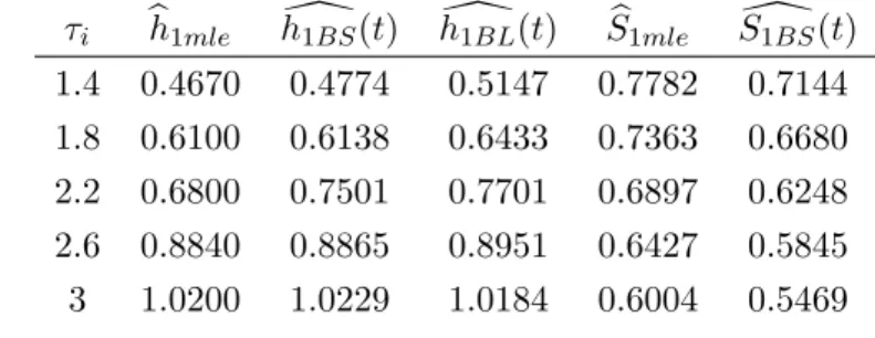
their lengths. Table 1 and Table 2 represent the Bayesian estimators for the specific survival and hazard functions with their corresponding maximum likelihood estimators of the hazard functions bh1mle, bh2_mle and the survival functions S1b mle, S2b_mle using the

ungrouped data at the end interval points for the two types of mechanical devises. As it appears from the Tables 1 and 2, the Bayesian estimators for both the spe-cific hazard and survival functions are also very close to their corresponding maximum likelihood estimators using the complete ungrouped data.

Taking into account that there is a specific loss of information in the exact life times when using the grouped data, the obtained Bayesian estimators indicates a high perfor-mance when using the competing risks grouped data.

8.2 Simulation

Because the maximum likelihood estimators using the complete ungrouped data in-corporate specific standard errors rates. In this section, using Matlab a Monte Carlo simulation study by proposing the true values of the parameters is conducted. Three modes of failure are considered with common shape parameter γ = 1.5 for the first setting, γ = 1 for the second setting and γ = 0.8 for the third setting. The proposed scale parameters areλ1= 0.1, λ2= 0.15, λ3= 0.20 with sample sizesn= 45,72,102 are generated from specific Weibull models; equal size subpopulations with rate of censoring 5%, 10% and 15% are considered. The generating data are grouped into 5 intervals with fixed length equal 1.5 and 7 intervals of fixed length equal 1 for the first setting, into 6 intervals with fixed length equal 3 and 8 intervals with fixed length equal 2.5 for the second setting and into 8 intervals with fixed length equal 5 and 10 intervals with fixed length equal 4 for the third setting. The prior scale parameter is fixed b = 2, and the shape parameters are a1 = 1.764, a2 = 2.647, a3 = 3.529 respectively, the LINEX loss parameter is fixed to be c = 2 in all the indices, for each setting 1000 replications of the life testing experiments are performed. The performance of the Bayesian estima-tors is measured in terms of their mean squared errors (MSE)and the mean percentage errors(MPE) defined respectively as:

M SE(λb_l) = 1 1000 1000 X i=1 (λi−λb_l)2 M P E(λb_l) = 1 1000 1000 X i=1 |λi−λb_l| λi whereλb_l is the Bayesian estimator of λ_i, i= 1,2,3.

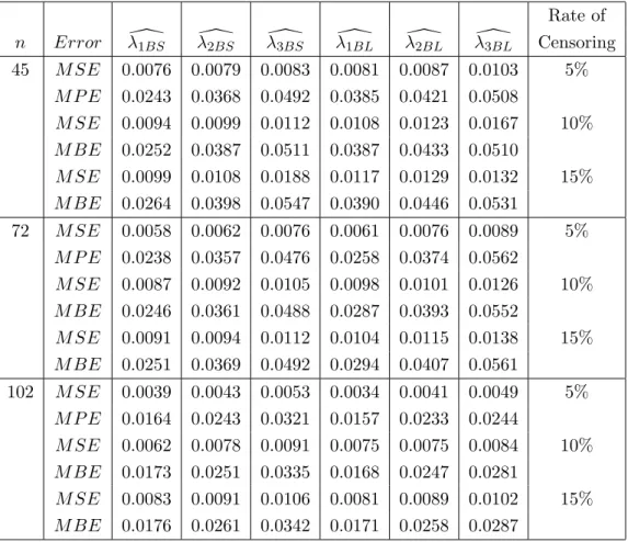
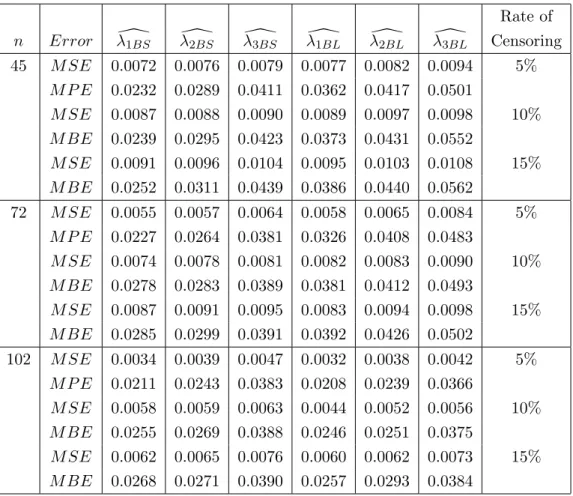
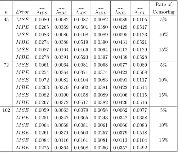
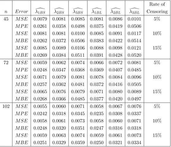
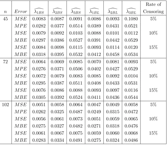
The MSEs and the MPEs of the Bayesian estimators at different settings are presented in the Tables 3, 4, 5, 6, 7 and 8 where we have the following results:

1. For fixed sample size, the MSEs and the MPEs of the Bayesian estimators uniformly increasing as the values of the parameters increasing. In Table 1, as the values of the parameter increasing from 0.1 to 0.2 the MSEs increasing from 0.0076 to 0.0083

(11)

using SELF and from 0.0081 to 0.0103 using LINEX. Similarly the MPEs increasing from 0.0243 to 0.0492 using SELF and from 0.0385 to 0.0508 using LINEX. 2. Following each column in the Tables, the MSEs and the MPEs of the Bayesian

decreasing as the sample sizes are increasing. Observation results also show that, the Bayesian estimators under SELF have less MSEs than the Bayesian estimators under LINEX when the sample sizesn= 45 and n= 72, the converse is not true when the sample sizen= 102.

3. Comparing the simulation results in Table 3 with Table 4 , Table 5 with Table 6 and Table 7 with Table 8, we realize that as the lengths of the inspection intervals decreasing and the number of intervals increasing, the Bayesian estimators become more efficient because it incorporate less MSEs and MPEs.

4. Comparing the simulation results in Table 3 and Table 4 with their corresponding results in Tables 5 and 6 and Tables 7 and 8, the Bayesian estimators are better when the shape parameter γ = 1.5 than the Bayesian estimators when γ = 1 and

γ = 0.8. This assigns that the Bayesian estimation approach is more preferable for the increasing failure rate process.

5. The rate of censoring can also be one of other factors affected performance of the Bayesian approach. Results with censoring rate 5% are significantly better than the results with censoring rates 10% and 15%.

6. Generally, simulation results show that, the derived Bayesian estimators are robust with respect to both scale and shape parameters and give a high performance as compared to the maximum likelihood and type moment estimators derived by Lianfen and Jose (2003).

9 Conclusion

In this article, Bayesian estimation approach is devoted for the Weibull parameters and related specific hazard and survival functions. Using the competing risks grouped data, the Bayesian estimators are obtained in explicit closed forms and not needed any numerical solutions. Applying the theoretical results to real lifetimes data manifest the performance of the Bayesian estimators as compared with their corresponding ordinary maximum likelihood estimators using the complete ungrouped data. Properties of the Bayesian estimators are studied through a simulation study which illustrates the factors that affected reliability of the estimation procedures. Being not having the exact failure times, the competing risks grouped data with the Bayesian estimation is recommended when continuous monitoring the test units is not feasible, costly or incorporates specific measurement errors.

(12)

References

Al-Salem, M., Almomani, M., Alrefaei, M., and Diabat, A. (2017). On the optimal com-puting budget allocation problem for large scale simulation optimization. Simulation Modelling Practice and Theory, 71:149–159.

Almomani, M. and Alrefaei, M. (2012). A three-stage procedure for selecting a good enough simulated system. Journal of Applied Probability and Statistics, 6(1&2):13–27. Almomani, M. and Alrefaei, M. (2016). Ordinal optimization with computing budget al-location for selecting an optimal subset. Asia-Pacific Journal of Operational Research, 33(2).

Almomani, M., Alrefaei, M., and Mansour, S. A. (2018). A combined statistical selection procedure measured by expected opportunity cost. Arabian Journal for Science and Engineering, 43(6):3163–3171.

Almomani, M. and R.AbdulRahman (2012). Selecting a good stochastic system for the large number of alternatives. Communications in Statistics-Simulation and Compu-tation, 41:222–237.

Alrefaei, M. and Almomani, M. (2007). Subset selection of best simulated systems.

Journal of the Franklin Institute, 344:495–506.

Aludaat, K., Alodat, M. T., and Alodat, T. (2008). Parameter estimation of burr type x distribution for grouped data. Applied Mathematical Sciences, 2(9):415–423. Alwasel, I. (2009). Statistical inference of a competing risks model with modified weibull

distributions. International Journal of Math Analysis, 3:905–918.

Berger, J. (1985). Statistical decision theory and Bayesian analysis. 2nd edition. Springer, New York.

Chambers, J., Cleveland, W., Kleiner, B., and Tukey, P. (1983). Graphical Methods for Data Analysis. Wadsworth, California.

David, H. and Moeschberger, M. (1978).The Theory of Competing Risks. Charles Griffn & Company, London.

Dey, A., Jha, A., and Dey, S. (2016). Bayesian analysis of modified weibull dis-tribution under progressively censored competing risk model. In arXiv preprint arXiv:1605.06585.

Gove, J. and Fairweather, S. (1989). Maximum likelihood estimation of weibull function parameters using a general interactive optimizer and grouped data. Forest Ecology and Management, 28(1):61–69.

Hamada, M., Reese, C., Wilson, A., and Martz, H. (2008).Bayesian Reliability. Springer, New York ,NY,USA.

Iskandar, I. and Gondokaryono, Y. (2016). Competing risk models in reliability systems, a weibull distribution model with bayesian analysis approach. In In IOP Conference Series: Materials Science and Engineering, volume 114, page 012064.

Josmar, M. and Jorge, A. (2011). Lindley distribution applied to competing risks lifetime.

(13)

Lai, C. and Murthy, D. (2003). A modified weibull distribution. IEEE Transaction on Reliability, 52(1):33–37.

Lai, X., Yau, K., and Liu, L. (2017). Competing risk model with bivariate random effects for clustered survival data. Computational Statistics & Data Analysis, 112:215–223. Lianfen, Q. and Jose, C. C. (2003). Estimation of the weibull parameters for grouped data

with competing risks. Journal of Statistical Computation and Simulation, 73:261–275. Lowe, P. and Lewis, W. (1983). Reliability analysis based on weibull distribution: an application to maintenance float factors.International Journal of Production Research, 21(4):461–470.

Migdadi, H. and Al-Batah, M. (2014). Bayesian inference based on the interval grouped data from the weibull model with application. British Journal of Mathematics & Computer Science, 4(9):1170–1183.

Mudholkar, G. and Asubonteng, K. (2010). Data-transformation approach to life-times data analysis: An overview. Journal of Statistical Planning and Inference, 140(10):2904–2917.

Pak, A. and Chatrabgoun, O. (2016). Inference for exponential parameter under progres-sive type-ii censoring from imprecise lifetime. Electronic Journal of Applied Statistical Analysis, 9(1):227–245.

Pak, A. and Rastogi, M. (2018). Classical and bayesian estimation of kumaraswamy distribution based on type-ii hybrid censored data. Electronic Journal of Applied Statistical Analysis, 11(1):235–252.

Pipper, C. and Ritz, C. (1989). Checking the grouped data version of the cox model for interval-grouped survival data. Scandinavian Journal of Statistics, 34(2):405–418. Prakash, G. (2014). Shift point bayes estimation under weibull failure model. Electronic

Journal of applied statistical analysis, 7(2):375–393.

Rinne, H. (2009). The Weibull Distribution. Chapman and Hall, USA.

Sarhan, A. M. (2007). Analysis of incomplete censored data in competing risks models with generalized exponential distributions. IEEE Trans in Reliability, 56:132–138. Shai, Y. and Wu, M. (2016). Statistical analysis of dependent competing risks model from

gompertz distribution under progressively hybrid censoring. Springer Plus, 5(1):1745. Tahir, M., Aslam, M., Hussain, Z., and Abbas, N. (2017). On the finite mixture of expo-nential raleigh and burr type-xii distributions: estimation of parameters in bayesian framework. Electronic Journal of applied statistical analysis, 10(1):271–293.

Varian, H. (1975). A bayesian approach to real estate assessment. Studies in Bayesian Econometric and Statistics in honor of Leonard J. Savage, pages 195–208.

Weibull, W. (1951). A statistical distribution function of wide applicability. Journal of Applied Mechanics, 18:293–297.

Yanez, S., Escobar, L., and Gonzalez, N. (2014). Characteristics of two competing risks models with weibull distributed risks. Revista de la Academia Colombiana de Ciencias Exactas, Fsicas y Naturales, 38(148):298–311.

(14)

center failures. Reliability Engineering and System Safety, 50(1):121–125.

Zellner, A. (1986). Bayesian estimation and prediction using asymmetric loss functions.

(15)

Table 1: The estimated hazard and survival functions of Type 1 mechanical devises. τi bh1_mle h1[BS(t) h1[BL(t) S1b _mle S1[_BS(t) 1.4 0.4670 0.4774 0.5147 0.7782 0.7144 1.8 0.6100 0.6138 0.6433 0.7363 0.6680 2.2 0.6800 0.7501 0.7701 0.6897 0.6248 2.6 0.8840 0.8865 0.8951 0.6427 0.5845 3 1.0200 1.0229 1.0184 0.6004 0.5469

Table 2: The estimated hazard and survival functions of Type 2 mechanical devises.

τi bh₁_mle h[₁_BS(t) h[₁_BL(t) Sb₁_mle S[₁_BS(t) 1.4 0.5392 0.5737 0.5846 0.7642 0.7515 1.8 0.8086 0.7376 0.7463 0.6681 0.6934 2.2 0.9882 0.9015 0.9058 0.6109 0.6269 2.6 1.1679 1.0654 1.0631 0.5585 0.5899 3 1.3476 1.2293 1.2183 0.5168 0.5451

(16)

Table 3: The mean squared errors and the mean percentage errors of the Bayesian esti-mators when the common shape parameter γ = 1.5,number of intervalsk= 5,

fixed interval length = 1.5.

Rate of n Error λ[1BS λ[2BS λ[3BS λ[1BL λ[2BL λ[3BL Censoring 45 M SE 0.0076 0.0079 0.0083 0.0081 0.0087 0.0103 5% M P E 0.0243 0.0368 0.0492 0.0385 0.0421 0.0508 M SE 0.0094 0.0099 0.0112 0.0108 0.0123 0.0167 10% M BE 0.0252 0.0387 0.0511 0.0387 0.0433 0.0510 M SE 0.0099 0.0108 0.0188 0.0117 0.0129 0.0132 15% M BE 0.0264 0.0398 0.0547 0.0390 0.0446 0.0531 72 M SE 0.0058 0.0062 0.0076 0.0061 0.0076 0.0089 5% M P E 0.0238 0.0357 0.0476 0.0258 0.0374 0.0562 M SE 0.0087 0.0092 0.0105 0.0098 0.0101 0.0126 10% M BE 0.0246 0.0361 0.0488 0.0287 0.0393 0.0552 M SE 0.0091 0.0094 0.0112 0.0104 0.0115 0.0138 15% M BE 0.0251 0.0369 0.0492 0.0294 0.0407 0.0561 102 M SE 0.0039 0.0043 0.0053 0.0034 0.0041 0.0049 5% M P E 0.0164 0.0243 0.0321 0.0157 0.0233 0.0244 M SE 0.0062 0.0078 0.0091 0.0075 0.0075 0.0084 10% M BE 0.0173 0.0251 0.0335 0.0168 0.0247 0.0281 M SE 0.0083 0.0091 0.0106 0.0081 0.0089 0.0102 15% M BE 0.0176 0.0261 0.0342 0.0171 0.0258 0.0287

(17)

fixed interval length = 1.

(18)

Table 5: The mean squared errors and the mean percentage errors of the Bayesian esti-mators when the common shape parameter γ = 1, number of intervalsk = 6,

(19)

Table 6: The mean squared errors and the mean percentage errors of the Bayesian esti-mators when the common shape parameter γ = 1, number of intervalsk = 8,

fixed interval length = 2.5.

(20)

(21)

Table 8: The mean squared errors and the mean percentage errors of the Bayesian esti-mators when the common shape parameterγ = 0.8,number of intervalsk= 10,