Vision-Based Reinforcement Learning using Approximate Policy
Iteration
Marwan R. Shaker, Shigang Yue and Tom Duckett
Abstract— A major issue for reinforcement learning (RL) applied to robotics is the time required to learn a new skill. While RL has been used to learn mobile robot control in many simulated domains, applications involving learning on real robots are still relatively rare. In this paper, the Least-Squares Policy Iteration (LSPI) reinforcement learning algorithm and a new model-based algorithm Least-Squares Policy Iteration with Prioritized Sweeping (LSPI+), are implemented on a mobile robot to acquire new skills quickly and efficiently. LSPI+ combines the benefits of LSPI and prioritized sweeping, which uses all previous experience to focus the computational effort on the most “interesting” or dynamic parts of the state space. The proposed algorithms are tested on a household vacuum cleaner robot for learning a docking task using vision as the only sensor modality. In experiments these algorithms are compared to other model-based and model-free RL algorithms. The results show that the number of trials required to learn the docking task is significantly reduced using LSPI compared to the other RL algorithms investigated, and that LSPI+ further improves on the performance of LSPI.
I. INTRODUCTION
Reinforcement learning from delayed rewards has been applied to mobile robot control in various domains. The ap-proach has been especially successful in applications where it is possible to learn policies in simulation and then transfer the learned controller to the real robot.However, applications involving learning on real robots are still relatively rare. In principle a mobile robot could learn any task from scratch by reinforcement learning, but learning of complex tasks can be very time consuming, so the researcher must find a way to speed up the learning. Techniques for accelerating reinforcement learning on real robots include (1) guiding ex-ploration by human demonstration, advice or an approximate pre-installed controller, (2) using replayed experiences or models to generate “simulated” experiences, and (3) applying function approximators for better generalization. Function approximators also provide a means for dealing with con-tinuous state and action spaces.
Many previous works on reinforcement learning in mo-bile robotics have applied value-based algorithms such as Q-learning, which estimate the long-term expected value of each possible action given a particular state. However when used with function approximators this approach can suffer from various problems including parameter-sensitive convergence behaviour, failure to converge in stochastic environments, sensitivity to perturbances, etc. [11]. Recent research in artificial intelligence has focused instead on Marwan R. Shaker, Shigang Yue and Tom Duckett are with the Department of Computing and Informatics, University of Lincoln, LN6 7TS Lincoln, United Kingdom
{mshaker,tduckett,syue}@lincoln.ac.uk
policy searchmethods, which perform direct search in policy space to determine the optimal policy.
This paper applies and extends a policy search algorithm called Least-Squares Policy Iteration (LSPI) [6]. The ap-proach is particularly suited to mobile robot applications as it has no learning rate parameters to tune and does not take gradient steps, meaning there is no risk of over-shooting, oscillation or divergence. The approach uses linear approximation to represent the state-action value function, followed by approximate policy improvement. This generally results in a small number of very large steps directly in policy space, whereas gradient-based policy search methods typically make a large number of relatively small steps to a parameterized policy function.
This paper presents an application of LSPI to learning control of a real mobile robot in a visual-servoing context. In addition, the paper introduces a model-based extension of LSPI that incorporates prioritized sweeping to further accelerate learning of new skills by mobile robots (LSPI+). Prioritized sweeping uses all previous experience to focus the computational effort on the most “interesting” or dynamic parts of the state space. Both algorithms, LSPI and LSPI+, were tested on a docking task using a Roomba mobile robot with vision as the only sensor and without explicit pose estimation, following the visual servoing framework introduced in [8]. The algorithms are compared to other state-of-the-art algorithms including Q-learning, Dyna-Q, Dyna-Q with prioritized sweeping (Dyna-Q+PS) and Dyna-Q with both prioritized sweeping and directed exploration (Dyna-Q+PS+DE). The results show that the number of trials re-quired to learn the docking task is significantly reduced using LSPI compared to the other RL algorithms investigated, and that LSPI+ further improves on the performance of LSPI.
II. RELATED WORK
Many authors have applied value-based reinforcement learning algorithms in mobile robotics. Weber and Zo-chios [13] proposed a neural network based approach for learning the docking task on a simulated robot with RL. Mart´ınez-Mar´ın and Duckett [8] proposed a model-based RL that accelerates the learning of docking on a real mobile robot. They used two controllers: a PD controller to extract the state variables from the vision sensors, and a RL con-troller which is used to drive the robot. Bakker et al. [2] introduce a model-based method based on Dyna-Q using prioritized sweeping, directed exploration and a transformed reward function to provide additional speed-ups on a real robot task, involving finding a specific object and moving towards that object while avoiding bumping into walls.
More recently various authors have applied policy search methods. Bagnell and Schneider [1] presented a gradient-based policy search method to learn control of a helicopter. Kwok and Fox [5] implemented LSPI on a simulated ball-kicking task in a soccer game, and used the trained controller in real robot experiments. Morimoto and Doya [9] applied a hierarchical RL method by which an appropriate sequence of sub-goals for the task is learned in the upper level while behaviors to achieve the subgoals are acquired in the lower level. Kolter et al. [4] used a similar state space representa-tion and proposed a method for hierarchical apprenticeship learning, which allows the algorithm to accept isolated advice at different hierarchical levels of the control task.
Our approach differs from the above approaches in that we learn the control policy from scratch on the real robot using only vision for state estimation, and that the time and number of trials required to learn the docking task is significantly reduced using approximate policy iteration.
III. OVERVIEW OF THE APPROACH A. Policy Iteration and Approximate Policy Iteration
Policy iteration consists of two phases: (1) policy evalu-ation, computing the value function Qπ(s, a) by solving a set of linear equations, and (2) policy improvement, using
Qπ(s, a) to find a better policy π0(a|s). Typically an e-greedy action selection policy is used to balance exploration of unknown parts of the state space and exploitation of the existing learned policy. It is known that repeating policy eval-uation and policy improvement results in the optimal policy
π∗ [12]. The convergence guarantee relies upon a tabular representation of the value function, and exact solution of the Bellman equations. However such representations and methods are impractical for large state and action spaces. In this case, approximation methods suggested by [6] are used, where the tabular representation of the policy π(s) of the Q-learning algorithm is replaced by a parametric function approximatorπˆ(s;θ), whereθ are the adjustable parameters of the representation, as shown in Fig 1. Policy iteration and approximate policy iteration in a high dimensional state space has been demonstrated previously in several papers [5], [6].
Fig. 1. Approximate Policy Iteration
B. Value function and approximate value function
In the evaluation phase of approximate policy iteration, the Q-value function needs to be updated, as shown in Fig 1. Even though policy iteration or approximated policy iteration is guaranteed to approach the optimal policy, a tabular representation of the state space will be impractical for real robot applications when the state space is very large or continuous, because the time required to reach the optimal policy will be infeasibly large. To overcome this dilemma, an approximated Q-value function is used instead of a tabular representation. The Q-value function is approximated by a parametric function Qˆπ(s, a;W), where W are the adjustable parameters of the approximator. The parametric function approximator Qˆπ(s, a;W) can be expressed as a linear weighted combination of a fixed number of basis functions as in Eq. 1. ˆ Qπ(s, a;W) = k X i=1 φi(s, a)wi= Φ(s, a)TW, (1)
where Φ(s, a) = (φ1(s, a), φ2s, a), ..., φk(s, a)) are fixed basis functions: each entry correspond to the basis function
φi(s, a) at the state-action pair (s, a), k is the number of basis functions and wi are the model parameters (weights). Note thatk |S| ∗ |A|.
C. Directed Exploration
One of the problems with RL algorithms is exploration when the agent does not have prior knowledge of the envi-ronment. By directing the exploration towards “interesting” parts of the state-action space (called Directed Exploration) and adding an exploration bonus (as shown in Eq. 2) to the Q-value function we gain a more efficient exploration technique than using undirected exploration [2].
Q(s, a)←Q(s, a) +εpm(s, a)/n(s, a), (2) whereε is a constant, m(s, a) is the number of time steps since action was first tried in states, andn(s, a)is the total number of times actiona was tried in state s. Ifn(s, a) is equal to zero it is replaced by one. This results in exploration that focuses on learning from actions that have been accessed more than other state-action pairs in that state.
IV. LSPI+ ALGORITHM
This section describes the basic components of LSPI+ (subroutines for model-free and model-based least-squares Q-learning, and prioritized sweeping).
A. Model-Free Least-Squares Q-Learning
The tabular representation can be rewritten as the orthog-onal set of basis functions φ(i) = [0, ...i, ...0]for each state in the state space. This representation is not efficient because it does not explain the topology of the specific state space. This problem requires more efficient approximations, such as the polynomial basis function used in this paper, where the Q-value functionQt(s)is approximated by a linear com-bination of the firstkelements of a sequence of polynomial
basis functions as shown in Eq. 1 defined over all s ∈ S. While this encoding is sparse, it is numerically unstable for a large state space [7]. But this numerical instability can be solved by scaling the values of φ. LSPI addresses these issues by using a function approximator with polynomial basis function instead of the tabular representation.
Assume that we have |A| actions in the current state s, and|S| is the total number of states. Thenφ will comprise
|A| vectors of k elements, where the first element of each vector is 1 and the remaining elements are calculated based on Eq. 3, with i from 1 tok.
φi(s, a) =φi−1(s, a)∗(10∗s)/S (3)
The benefits from using linear approximation methods to represent the state space as a combination of k basis func-tions (features) can be viewed as performing dimensionality reduction: the linear approximation methods approximate the state-action value function Qπ(s,a) for the policy π using a set of hand coded basis functions φ(s,a), which reduces the vector Qπ(s,a) in high dimensional space R|S|∗|A|to Rk wherekis some fixed number usually equal to the order of the polynomial plus one, k | S | × |A | [6], [7]. This dimensionality reduction is used to generalize the obtained experience from a small subset of the state space to a larger subset of the state space.
Using Eq. 1 to approximate the state-action value function, let Qπ be a real vector ∈ R{|S|∗|A|}. The approximated action-state value function can be written as Qπ = ΦWπ, whereWπ is a vector of lengthk. Each row ofΦspecifies all the basis functions for a particular state action pair(s, a), and each column represents the values of particular basis function over all state-action pairs(s, a).
Using Eq. 1 with the Bellman backup operator yields the following solution for the coefficient (see [6] for proof):
Wπ= (ΦT(Φ−γPY
π
Φ))−1ΦTR, (4)
where P is a stochastic matrix that contains the transition model of the process, and R is a vector that contains the reward values.
Now, we need to calculate the values ofW, but the values of P and R will be unknown or too large to be used in practice. To overcome this problem, we need to solve the linear system of equationsGWπ =bto obtain the required
Wπ. The value of Wπ can be calculated by solving the following linear system of equations [6]:
G = ΦT∆µ(Φ−γP
Y
π
Φ), (5)
b = ΦT∆µR, (6) where µ is the probability distribution over (S×A) that defines the weights of the projection. But the values ofGand
bare unknown or very large also becauseP andRare either large or unknown, so we will use the least-squares fixed point approximation to learn the state-action value function
of a fixed policy from samples as in Eqs. 7 and 8, which is equivalent to the learning of parameterWπ ofQπ= ΦWπ.
˜ Gt+1 = G˜t+φ(st, at)(φ(st, at)−γφ(s0t, π(s0t))) T, (7) ˜ bt+1 = ˜bt+φ(st, at)rt, (8) where (st, at, rt, s0t) is the t
th sample of experience from a trajectory generated by the agent. The computation of G,
b based on samples and the resulting Wπ by solving the linear system of equationsGWπ=b is called least-squares Q-learning (LSQ), which is repeated for some number of iterations or until the algorithm converges.
TABLE I
LSQMODEL-FREE ALGORITHM
Function LSQ model-free(SS, k,φ,γ,π)
SS: set of samples (s, a, r, s’), k: number of basis functions
φ: Basis function,γ: Discounted factor,π: Policy 1. G→Zero, b→Zero
2. for each sample(s, a, r, s’) perform equation 7 & 8 3. Wπ= G−1 b
4. return Wπ
B. Model-Based Least-Squares Q-Learning
A classical model-based algorithm to learn Qπ from simulated trajectory data can be explained as follows [3].
1) From the state transitions and rewards observed so far, build in memory an empirical model of the Markov chain. The sufficient statistics of this model are as follows:
a) A vector n recording the number of times each state has been visited.
b) A matrix C recording the observed state-transition counts: Cij i.e. how many times state
xi is changed directly to statexj.
c) A vectorurecording the sum of all observed one-step rewards from each state.
2) Whenever a new estimate of the state-action value functionQπis desired, solve the linear system of Bell-man equations corresponding to the current empirical model, where N is a diagonal matrix of the vectorn, then the solution vector of the empirical model is
(N−C)−1u (9) The model links each state to all the downstream states that follow that state on any trajectory, and records how much each state has influence on the other states. All this can be viewed as doing two steps:
1) Each state is visited, C and u are updated and a Markov chain is built from that state to every possible other state.
2) The chain compactly models all the backups performed on the data. As shown in Eq. 10, each time the state-action pair is visited, theGandbmatrices are updated based on the changes in the model.
The proposed model does not maintain any statistics on observed transitions and rewards, it just updates the compo-nents of Eq. 9 directly. The advantage of the model-based method is that it makes the most of the available training data.
It is clear that the role of b is the sum of all reward received, which is exactly the same as the vector u in the proposed model. The outer product from Eq. 7 is a sparse matrix. Summing such a sparse matrix for each observed transition givesG≡N−C.
G= ΦT(N−C)Φ , b= ΦTs (10) Matrices G and b effectively record a model of all the observed transitions. In this case, we can view LSQ as implicitly building a compressed version of the empirical model’s transition matrix (N −C) and summed-reward vector u, and the resulting G and b from Eq. 10 can be written as shown in Eqs. 11 and 12.
˜
Gt+1 = G˜t+φ(st, at)(Nt−Ct)φ(st, at)T (11) ˜bt+1 = ˜bt+φ(s
t, at)st (12) If(N−C)is singular, we can write(N−C)in a different format N −C = N(I−N−1C), where I is the identity
matrix. Now if we impose kN−1Ck < 1 then the matrix
(N−C)is always non-singular. But if (N−C)is singular then Singular Value Decomposition (SVD) [10] can be used to find the solution where the dependant columns correspond to a smaller singular value that can be omitted to find the solution.
C. Model-Based Least-Squares Q-Value with Prioritized Sweeping
In RL, state transitions are stored in state-action pairs that may be selected uniformly at random from all previously ex-perienced pairs, but uniform selection is usually not the best method; planning can be much more efficient if simulated transitions and backups are focused on particular state-action pairs [12], [2]. The number of state-action pairs backed up often grows rapidly, producing many pairs that could usefully be backed up. But not all of these will be equally useful: the important parts of the state that have changed a lot are also more likely to change a lot, whereas others will change little [12].
By prioritizing the state-action pairs based on the number of times the state-action pair has been visited and based on the transition from one pair to another pair, each time state
s is visited the value of the state-priority for that state is increased by one. The final prioritypfor that state-action pair is shown in Eq. 13, withp >0 as threshold. Table I shows the free LSQ algorithm [6], while Table II shows model-based LSQ.
p=reward+(γQ(s0, a0)−Q(s, a))∗state−priority (13)
TABLE II
LSQMODEL-BASED ALGORITHM
Function LSQ model-based(SS, k,φ,γ,π)
SS: set of samples (s, a, r, s’), k: number of basis functions
φ: Basis function,γ: Discounted factor,π: Policy 1. G→Zero , b→Zero
2. prioritize n and C based on their values 3. for each sample (s, a, r, s’)
perform Eq. 11 & 12 4. Wπ= G−1 b
5. return Wπ
D. Model-Based LSPI with Prioritized Sweeping
LSPI+ combines the policy search efficiency of policy iter-ation and data efficiency of Least-Squares Q-learning (LSQ) with the efficient back-up of state-action pairs of prioritized sweeping. The LSQ algorithm provides a means of learning an approximate state-action value function, Qπ(s,a), for any fixed policy [6]. By integrating LSQ and the empirical model into an approximate policy iteration algorithm we obtain the LSPI+ algorithm, which is summarised in Table III.
TABLE III
LSPIMODEL-BASED ALGORITHM
Function LSPI Model-based (S, k,φ,γ,π)
SS: set of samples (s, a, r, s’), k: number of basis functions
φ: Basis function,γ: Discounted factor,π: Policy 1. i←Zero, w0←initialize weights to zero
2. Repeat a. i = i +1
b. wi= LSQ(SS, k,φ,γ,π)
c. repeat for N times
wi= LSQModel(SS, k,φ,γ,π)
3. Untilkwi+1-wik< or i>imaximum
4. return Wπ
V. EXPERIMENTS
The performance of the introduced LSPI+ and LSPI algo-rithms are investigated and compared to Q-learning, Dyna-Q, Q with prioritized sweeping (Q+PS), and Dyna-Q with prioritized sweeping and directed exploration (Dyna-Q+PS+DE) on a docking task.
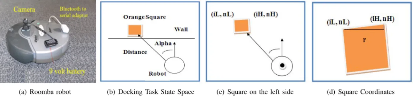
In our experiments, a Roomba vacuum cleaner robot was used for the docking task using vision only for state estimation. To simplify the detection process, an artificial landmark consisting of an orange square was used to mark the goal for the docking task. As shown in Fig 2(a), the robot was equipped with a low-cost wireless camera (powered by a 9 volt battery) used to send images to an off-board computer. A Bluetooth to serial adapter was used to send commands back from the off-board computer to the robot. In the docking task, the robot has two actions: either turn left or turn right, while driving forwards at a constant speed.
A. Docking Task and State Space Representation
The docking task given to the robot consists of starting from a random position in the vicinity of a docking station and driving while steering itself towards a desired configura-tion at the docking staconfigura-tion. The docking staconfigura-tion is not defined
(a) Roomba robot (b) Docking Task State Space (c) Square on the left side (d) Square Coordinates Fig. 2. Orange Square on the left side of the captured image.
TABLE IV DOCKINGTASKPARAMETERS
State Variables Alpha: [−80
o,80o] sampled every 10 degrees
Distance :[0,3] meter sampled every 0.2 meter
Reward
reward =100 if it gets to the goal
reward =-50 if it finishes outside state space reward equal to a value, this value is decrease as the number of the steps to the goal increases Goal State (alpha, distance) = ([−5o,5o],[0,180] mm)
Control Variables Vr (Rotational Velocity)is fixed to either -5o/s or 5o/s
beforehand as a known robot location. On the contrary it is specified as a set of sensor perceptions obtained from this station. In our experiments we used a vision system to detect an orange square used to mark the docking station.
We used a state space consisting of two variables: alpha and distance. Alpha is the angle between the robot heading direction and the line that is pointing from the central position of the robot to the orange square. Alpha and distance are calculated from the vision system information. Table IV summarizes the state space representation.
B. Distance and Alpha calculation using the vision system On initialization, the robot attempts to detect the orange square. If it is not detected then the robot rotates at 10 degree intervals until part of the orange square becomes visible.
The state variables Alpha and Distance are then calculated as follows. As shown in Fig. 2(c), the location of the upper left corner of the square is (iL, nL) and the upper right corner is (iH, nH). The distanceras shown in Fig. 2(d) is equal to the number of orange columns between the two points. We then calculate the angle Alpha as:
Alpha= cos−1(p r
(iH−iL)2+ (nH−nL)2) (14)
The Distance variable is estimated from the number of columns and rows inside the orange square in the image. This is done by simple linear interpolation. We captured one image when the robot distance from the orange square was one meter and we captured a second image when the robot distance was 2 meters. In both captured images we calculate the number of columns and rows, then for new images we obtain Distance by interpolating on the stored values for 1 and 2 meters.
C. Simulated Results
The simulated experiments were performed using Mo-bileSim (http://robots.mobilerobots.com/wiki/MoMo-bileSim). In the simulated environments the docking station is defined by a box and the robot has to learn how to move toward this box and dock to a goal state, as specified in Table IV, using two actions (turn right or turn left) while the robot moves forward with a constant velocity starting from a random position in the environment.
The previously described algorithms were compared using the percentage of successful docking attempts versus the number of learning trials. For all the algorithms, after every 5 trials of learning we stopped the learning and performed 100 trials without learning, calculating the proportion of successful trials. The results are shown in Fig. 5. As can be
Fig. 5. Simulated results showing the percentage of successful docking attempts against the number of learning trials.
seen in Fig. 5 the performance of Q-learning is the worst of all algorithms, and the performance gets better for Dyna-Q, Dyna-Q+PS and Dyna-Q+PS+DE respectively. Model-free LSPI gives better performance than the above algorithms, where it took about 31 trials to get near the maximum value obtained by LSPI+, while LSPI+ gets the best results with 25 trials to get to the maximum percentage of successful trials. In comparison Q-learning took 223 trials to get to 80% and Dyna-Q took 180 trials to get to 80%.
D. Real Robot Experiments
LSPI+ and LSPI were tested for the proposed state space. The state space is represented by using a polynomial of order 2 and 4: for the case of 2 this means that the fixed number k for the linear architectural representation equals 3, but LSPI+ and LSPI required more than 27 iterations to converge for each state and sometimes did not select to the correct value, while for the polynomial of order 4, this means that the fixed number k for the linear architectural representation equals
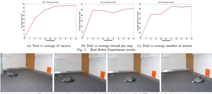
(a) Trial vs average of success (b) Trial vs average reward per step (c) Trial vs average number of actions Fig. 3. Real Robot Experiments results.
Fig. 4. sequence of images showing the docking behavior learned by LSPI+ on the real robot. 5, and LSPI and LSPI+ required more than 3 iterations to
converge for each state. So we used in our experiments the polynomial of order 4, and with initial policy exploration equal to 40 percent ( = 0.4), a discount factor of 0.9, total number of actions equal two and zero initial weights. For the convergence criterion we set = 0.001 with at least 5 steps for each trial (we checked for more than 5 steps and found no difference in the performance of the algorithm and sample collection). The results of the Roomba robot training can be summarized as follows: for LSPI+ after 28 trials of learning (taking 29 minutes), the robot was able to dock to the orange square from any location within the state space, while model-free LSPI required 33 trials (taking 35 minutes). Fig. 4 shows an image sequence of the docking behaviour obtained using LSPI+ after 30 trials of learning. Fig. 3 show the results of the LSPI+ experiments (including the percent-age of successful attempts to reach the goal in Fig. 3(a), the average reward received per step in Fig. 3(b) and the average number of actions taken to get to the goal in Fig. 3(c), where after every 10 trials of learning we stopped the learning and performed 50 trials without learning, calculating the three performance measures for those 50 trials.
VI. CONCLUSION ANDFUTURE WORK
This paper implemented the LSPI algorithm on a real mobile robot docking task and also introduced model-based LSPI with prioritized sweeping (LSPI+). The experiments and simulated results demonstrate that the performance of LSPI and LSPI+ is significantly better than the other algo-rithms investigated in terms of both time and trials required to learn the docking task. LSPI and LSPI+ found the optimal policy faster than traditional techniques with fewer samples, evaluating the policy in a single pass over the collected samples. There is also a modest improvement in performance using LSPI+ compared to LSPI. We understand this to be a ceiling effect where both algorithms are already close to the best possible performance on the vision-based docking task. In future work we will investigate tasks with
higher-dimensional continuous state spaces to further evaluate the performance of the proposed algorithm.
VII. ACKNOWLEDGEMENT
The authors would like to acknowledge the support of both Lincoln University and the Council for Assisting Refugee Academics (CARA).
REFERENCES
[1] J. A. Bagnell and J. G. Schneider. Autonomous helicopter con-trol using reinforcement learning policy search methods. InProc. ICRA Robotics and Automation IEEE International Conference on, volume 2, pages 1615–1620, 2001.
[2] B. Bakker, V. Zhumatiy, G. Gruener, and J. Schmidhuber. Quasi-online reinforcement learning for robots. InProc. IEEE International Conference on Robotics and Automation ICRA 2006, 2006. [3] Justin A. Boyan. Least-squares temporal difference learning. In
Machine Learning: Proceedings of the Sixteenth International Con-ference. Morgan Kaufmann, 1999.
[4] J. Zico Kolter, Pieter Abbeel, and Andrew Ng. Hierarchical apprentice-ship learning with application to quadruped locomotion. In J.C. Platt, D. Koller, Y. Singer, and S. Roweis, editors, NIPS 20, Cambridge, MA, 2008. MIT Press.
[5] C. Kwok and D. Fox. Reinforcement learning for sensing strategies. InProc. IEEE/RSJ International Conference on Intelligent Robots and Systems (IROS 2004), volume 4, pages 3158–3163, 2004.
[6] Michail G. Lagoudakis and Ronald Parr. Least-squares policy iteration.
Journal of Machine Learning Research, 4:2003, 2003.
[7] Sridhar Mahadevan. Representation policy iteration. Proceedings of the 21st Conference on Uncertainty in AI (UAI-2005), Edinburgh, Scotland, July 26-29, 2005.
[8] T. Martinez-Marin and T. Duckett. Fast reinforcement learning for vision-guided mobile robots. InProc. IEEE International Conference on Robotics and Automation ICRA 2005, pages 4170–4175, 2005. [9] Jun Morimoto and Kenji Doya. Acquisition of stand-up behavior by
a real robot using hierarchical reinforcement learning. Robotics and Autonomous Systems, 36(1):37–51, 2001.
[10] William H. Press, Saul A. Teukolsky, William T. Vetterling, and Brian P. Flannery. Numerical Recipes in C++: The Art of Scientific Computing. Cambridge University Press, February 2002.
[11] Richard S. Sutton, David Mcallester, Satinder Singh, and Yishay Man-sour. Policy gradient methods for reinforcement learning with function approximation. In In Advances in Neural Information Processing Systems 12, pages 1057–1063. MIT Press, 2000.
[12] R.S. Sutton and A.G. Barto.Reinforcement Learning: An Introduction. MIT Press, 1998.
[13] Cornelius Weber, Stefan Wermter, and Alexandros Zochios. Robot docking with neural vision and reinforcement. Knowledge-Based Systems, 17:165–172, 2004.