Does Twitter predict Bitcoin?
Article
Accepted Version Creative Commons: AttributionNoncommercialNo Derivative Works 4.0Shen, D., Urquhart, A. and Wang, P. (2019) Does Twitter
predict Bitcoin? Economics Letters, 174. pp. 118122. ISSN
01651765 doi: https://doi.org/10.1016/j.econlet.2018.11.007
Available at http://centaur.reading.ac.uk/80420/
It is advisable to refer to the publisher’s version if you intend to cite from the work. See Guidance on citing . To link to this article DOI: http://dx.doi.org/10.1016/j.econlet.2018.11.007 Publisher: Elsevier All outputs in CentAUR are protected by Intellectual Property Rights law, including copyright law. Copyright and IPR is retained by the creators or other copyright holders. Terms and conditions for use of this material are defined in the End User Agreement .www.reading.ac.uk/centaur
CentAUR
Central Archive at the University of Reading
Reading’s research outputs online1
Does Twitter Predict Bitcoin?
Abstract
This paper adds to the growing literature of Bitcoin by examining the link between investor attention and Bitcoin returns, trading volume and realized volatility. Unlike previous studies, we employ the number of tweets from Twitter as a measure of attention rather than Google trends as we argue this is a better measure of attention from more informed investors. We find that the number of tweets is a significant driver of next day trading volume and realized volatility which is supported by linear and nonlinear Granger causality tests.
2
1. Introduction
Bitcoin has received extensive attention in the academic literature since it first introduced by Nakamoto in 2008, as demonstrated by the recent review paper by Corbet et al (2018). Bitcoin is the most popular cryptocurrency in terms of trading volume and is a peer-to- peer electronic cash system which allows online payments to be sent directly from one party to another without going through a financial institution. Therefore unlike the vast majority of other financial assets, Bitcoin have no association with any higher authority, such as a government, firm, country or commodity. Bitcoin also has no physical representation and its value is based on the security of an algorithm which is able to trace all transactions between buyers and sellers. Cryptocurrencies have received lots of media attention as well as investor attention, which is due to their low transaction costs, peer-to-peer system and governmental free design. This has led to a surge in trading volume, volatility and price of cryptocurrencies, with cryptocurrencies regularly in the mainstream news. A strand of literature has examined whether Bitcoin returns are predictable, with Urquhart (2016) indicating that Bitcoin returns are predictable and therefore are contrary to the Efficient Market Hypothesis. This finding has been further supported by Nadarajah and Chu (2017), Tiwari et al (2018), Kjuntia and Pattanayak (2018) and Caporale et al (2018) amongst others. All of these papers examine the relationship between returns and whether there are patterns or correlations that may be exploitable by investors. A recent paper by Urquhart (2018) shows that the attention of Bitcoin, captured by Google Trends, can be explained by the previous days realized volatility and volume, indicating that the high volatility and trading volume experienced by Bitcoin number of times the term ‘Bitcoin’ has been searched for in the Google search engine, and therefore is a good measure of attention from uninformed individuals who want to find out more information about Bitcoin. However well-informed investors, who have knowledge of the cryptocurrency, will not be searching for it in the Google search engine but instead may be tweeting about it. These tweets may involve commenting on news posts related to Bitcoin or making predictions of the future price direction of Bitcoin or just giving an opinion of the popular cryptocurrency. Hence we postulate that the volume of Bitcoin tweets is a stronger measure of investor attention than Google Trends, which we suggest is a measure uninformed investor attention.
There is a growing literature examining the impact of Twitter on financial markets, such as Piñeiro-Chousa et al (2016), Sun et al (2016 and Piñeiro-Piñeiro-Chousa et al (2018) who all find significant relationships between Twitter and financial markets. We add to this literature by being the first to study whether the volume of tweets involving the term ‘Bitcoin’ can predict the returns, volatility and trading volume of Bitcoin. This measure of investor attention should be more informed than that of Google Trends and therefore may reflect the attention Bitcoin is receiving from more informed investors. We find that the volume of tweets are significant drivers of realized volatility (RV) and trading volume, which is supported by linear and nonlinear Granger causality tests. However, we find no significant evidence that previous days tweets significantly influence the returns of Bitcoin. Therefore we add to the literature on the relationship between social media attention and Bitcoin.
2. Data and methodology
We obtain Twitter data on Bitcoin from https://bitinfocharts.com/, which captures the number
of times the term ‘Bitcoin’ has been tweeted and we study the period 4th September 2014 to 31st
August 2018 due to data availability. We download Bitstamp exchange tick data from
www.bitcoincharts.com, as it is one of the most popular and liquid Bitcoin exchanges. From the tick data, we aggregate up to the daily level and calculate logarithmic returns and trading volume. Figure 1 presents the time-series graph of the price of Bitcoin where we can see the huge surge
3
in price during the second half of 2017 and the subsequent falling of price during 2018. In order to measure daily RV, we aggregate the tick data up the 5-minute level such that:
𝑅𝑉# = %& 𝑟#,)* +
),-(1)
where 𝑟#,)* is squared 5-minute log returns of Bitcoin at day t during the interval j and n is the
number of intraday return intervals. We calculate returns over the 5-minute frequency to avoid well-known microstructure issues while we also obtain daily volume and returns by aggregating the tick data up to the daily level. Similar to Urquhart (2018), we take the logarithmic returns, realized volatility, trading volume as well as number of tweets to avoid large skewness and excess kurtosis. Table 1 provides the descriptive statistics where the log-tweets data which shows a maximum value of 11.96 and minimum of 8.90, with positive skewness and a leptokurtic distribution. The mean is 10.32 indicating that each day, there is a sufficient number of tweets
about Bitcoin during our sample period. The mean of the RV is −3.31, with quite a large standard
deviation of 0.52 as well as positive skewness. The mean log-volume indicates quite high liquidity in the Bitcoin market, with a maximum log-volume of 11.73 and minimum of 6.58. Returns over our sample period are positive, with negative skewness and excess kurtosis.
To examine the dynamics between our Bitcoin variables and the number of tweets, we estimate a
vector autoregressive (VAR) model, where 𝑥# is a vector that contains the variables of interest and
a VAR(k) model is:
𝑥# = c + & 𝛽)𝑥#2)+ 𝜀#
4
),-(2)
Where c is a vector of constants and 𝜀# is a vector of independent white noise innovations. The
lag length is determined by the Schwarz Bayesian information criterion and we estimate three separate models examining whether the volume of tweets can help predict realized volatility, trading volume and Bitcoin returns separately. From these VAR models, we employ the linear Granger causality test (Granger 1969) as well as the nonlinear causality test of Diks and Panchenko (2006). The linear Granger causality test can be expressed as:
∆𝑥#= 𝛽6 + & 𝛽-7∆𝑥#2-+ & 𝛽*7∆𝑦#2-+ 𝜀-# 9 7,-: 7,-∆𝑦# = 𝛿6+ & 𝛿-7∆𝑦#2-+ & 𝛿*7∆𝑥#2-+ 𝜀*# 9 7,-: 7,-(3)
Where the lag length is determined by the Schwarz Information Criterion.1
3. Empirical Results
1 We do not provide details of the nonlinear Granger causality test of Diks and Panchenko (2006) due to space
4
Table 2 reports the VAR models where the coefficient estimates are reported in Panel A and the two Granger causality results are reported in Panels B and C respectively. We can see from Model (1), which examines the relationship between RV and tweets, that the previous days tweet has a significant influence on RV indicating that higher the number of tweets, the higher the next day’s RV. This is supported by the linear and nonlinear Granger causality results which both suggest that we can reject the null hypothesis that tweets do not Granger cause RV. We also find that previous day’s RV has a significant influence on next day’s tweets, indicating a bilateral relationship which is supported by both Granger causality tests. We also find similar results for trading volume where previous tweets have a significant impact on trading volume while both linear and nonlinear Granger causality tests support this finding, indicating that higher tweets on Twitter significantly influences the next RV, trading volume. This also find that this is bilateral relationship too where previous volume significantly influences tweets. For returns, we find weak evidence (statistically significant at the 10% level) that less tweets have a relationship next day returns, although both Granger causality tests provide significant evidence that tweets do Granger cause returns. However we do not find any significant relationship between previous returns and tweets, indicating that the link between returns and tweets is a unilateral relationship.
Therefore our initial results indicate that previous days tweets do Granger cause RV and trading volume. However the price and behaviour of Bitcoin has changed drastically over time and therefore our findings in Table 2 may not be stable over time. Therefore we split our sample into two subsamples, where the breakpoint is determined by the Bai and Perron (2003) test. The breakpoint with the greatest significance is chosen which generates are new subsample periods,
which runs from 4th September 2014 to 8th October 2017, while the second subsample period
spans from 9th October 2017 to 31st of August 2018. The results for the two subsample periods
are reported in Tables 3 and 4 respectively where we find that in the first subsample, previous tweets have a significant effect on volume but not for RV, with both results supported by their respective Granger causality results. Consequently in the first subsample period, tweets to Granger cause volume, but not RV. However in the second subsample period, we find that previous tweets do have a significant effect on RV and volume, which are both supported by significant linear and nonlinear Granger causality results. Therefore we show that previous tweets do cause a significant increase in RV and volume the next day, which is only significant in our second subsample period.
4. Conclusion
This paper studies the relationship between the number of tweets referring to Bitcoin and whether they are useful in forecasting future RV, volume or returns. We find that the number of previous day tweets are significant drivers of Bitcoin RV and volume, but not returns. After splitting our sample into two subsample periods, we find that tweets only significantly influence volume in the first sample, but significantly influences both RV and volume in the second subsample period. Therefore we show that the number of tweets on Twitter can significantly predict future RV and trading volume of Bitcoin.
5
References
Bai J, Perron P. (2003). Computation and analysis of multiple structural change models. Journal of
Applied Econometrics, 18, 1-22.
Caporale, G. M., Gil-Alana, L., Mestel, R. (2018). Persistence in the cryptocurrency market. Research
in International Business and Finance, 46, 141-148.
Corbet, S., Lucey, B., Urquhart, A., Yarovaya, L. (2018). Cryptocurrencies as a Financial Asset: A
systematic analysis. International Review of Financial Analysis, forthcoming.
Diks C, Panchenko V. (2006). A new statistic and practical guidelines for nonparametric Granger
causality testing. Journal of Economic Dynamics and Control, 30, 1647-1669.
Granger, C. (1969). Investigating casual relations by econometric models and cross-spectral
methods. Econometrica, 37, 424-438.
Kjuntia, S., Pattanayak, J. (2018). Adaptive market hypothesis and evolving predictability of bitcoin.
Economics Letters, 167, 26-28.
Nadarajah, S., Chu, J. (2017). On the inefficiency of bitcoin. Economics Letters, 150, 6-9.
Piñeiro-Chousa, J., López-Cabarcos, A. A., Pérez-Pico, A. M. (2016). Examining the influence of
stock market variables on microblogging sentiment. Journal of Business Research, 69(6), 2087-2092.
Piñeiro-Chousa, J., López-Cabarcos, A. A., Pérez-Pico, A. M., Ribeiro-Navarrete, B. (2018). Does social network sentiment influence the relationship between the S&P 500 and gold returns?
International Review of Financial Analysis,57, 57-64.
Sun, A., Lachanski, M., Fabozzi, F. J. (2016). Trade the tweet: Social media text mining and sparse
matrix factorization for stock market prediction. International Review of Financial Analysis, 48,
272-281.
Tiwari, A. K., Jana, R., Das, D., Roubaud, D. (2018). Informational efficiency of bitcoin – an
extension. Economics Letters, 163, 106-109.
Urquhart, A. (2016). The inefficiency of Bitcoin. Economics Letters, 148, 80-82.
6
Mean Std. Dev Max Min Skewness Kurtosis
Log-Tweet 10.3242 0.4712 11.9550 8.8956 0.7599 0.2484
Log-RV -3.3053 0.5158 -1.0836 -4.6537 0.4922 0.2690
Log-Volume 9.0548 0.7532 11.7296 6.5781 -0.0798 0.0361
Log-Ret 0.0023 0.0391 0.2384 -0.2809 -0.2825 6.2127
Table 1: The descriptive statistics of the log number of Tweets, log RV, log volume and log returns.
7
Model (1) Model (2) Model (3)
𝑅𝑉# 𝑇𝑤𝑒𝑒𝑡# 𝑉𝑜𝑙𝑢𝑚𝑒# 𝑇𝑤𝑒𝑒𝑡# 𝑅𝑒𝑡# 𝑇𝑤𝑒𝑒𝑡# Constant -0.9014*** 0.1806 0.7650*** 0.3302*** -0.0355 0.2030** 𝑇𝑤𝑒𝑒𝑡#2- 0.1359*** 0.4543*** 0.3344*** 0.5531*** -0.0104* 0.4666*** 𝑇𝑤𝑒𝑒𝑡#2* -0.0083 0.0560** -0.0694 0.1061*** -0.0013 0.0601** 𝑇𝑤𝑒𝑒𝑡#2J -0.1030* 0.0078 -0.2721*** 0.0307 0.0108 0.0036 𝑇𝑤𝑒𝑒𝑡#2K 0.0431 0.0155 -0.0242 0.0725** -0.0002 0.0153 𝑇𝑤𝑒𝑒𝑡#2L -0.0219 0.0824*** 0.1204 0.2132*** -0.0060 0.0760*** 𝑇𝑤𝑒𝑒𝑡#2M 0.0639 0.1217*** 0.0041 0.1197*** 𝑇𝑤𝑒𝑒𝑡#2N -0.0659 0.2445*** 0.0067 0.2391*** 𝑅𝑉#2- 0.5846*** 0.0276** 𝑅𝑉#2* 0.0777*** -0.0030 𝑅𝑉#2J 0.0443 -0.0062 𝑅𝑉#2K 0.0474 0.0059 𝑅𝑉#2L 0.0035 -0.0278* 𝑅𝑉#2M 0.0990*** 0.0080 𝑅𝑉#2N 0.0088 -0.0062 𝑉𝑜𝑙𝑢𝑚𝑒#2- 0.5371*** 0.0306*** 𝑉𝑜𝑙𝑢𝑚𝑒#2* 0.0088 -0.0301*** 𝑉𝑜𝑙𝑢𝑚𝑒#2J 0.1175*** 0.0036 𝑉𝑜𝑙𝑢𝑚𝑒#2K 0.0681** -0.0134 𝑉𝑜𝑙𝑢𝑚𝑒#2L 0.0819*** 0.0007 𝑅𝑒𝑡#2- -0.0112 -0.0044 𝑅𝑒𝑡#2* -0.0186 -0.0121 𝑅𝑒𝑡#2J 0.0436 0.1501 𝑅𝑒𝑡#2K -0.0323 0.1102 𝑅𝑒𝑡#2L 0.0037 0.0182 𝑅𝑒𝑡#2M 0.0440* 0.0213 𝑅𝑒𝑡#2N 0.0091 0.0964
Panel B: Linear Granger Causality
RV does not Granger cause Tweets 4.024** Tweets does not Granger cause RV 8.434*** Volume does not Granger cause Tweets 4.471** Tweets does not Granger cause Volume 8.398*** Ret does not Granger cause Tweets 2.202 Tweets does not Granger cause Ret 6.001*** Panel C: Nonlinear Granger Causality
RV does not Granger cause Tweets 1.824** Tweets does not Granger cause RV 2.786*** Volume does not Granger cause Tweets 1.394* Tweets does not Granger cause Volume 2.544*** Ret does not Granger cause Tweets 0.011 Tweets does not Granger cause Ret 1.806**
Table 2: This table reports the VAR estimation results for the full sample period where each model examines the relationship between the number of tweet and RV, volume and returns respectively. The lag length is selected by the Schwarz Information Criterion. In Panels B and C, we report the linear Granger causality results, as well as the nonlinear Granger causality test of Diks and Panchenko (2006). ***, **, * indicate significance at the 1%, 5% and 10% levels respectively.
8
Model (1) Model (2) Model (3)
𝑅𝑉# 𝑇𝑤𝑒𝑒𝑡# 𝑉𝑜𝑙𝑢𝑚𝑒# 𝑇𝑤𝑒𝑒𝑡# 𝑅𝑒𝑡# 𝑇𝑤𝑒𝑒𝑡# Constant -0.4762 0.2850* 0.8095* 0.5942*** -0.0550* 0.3037** 𝑇𝑤𝑒𝑒𝑡#2- 0.0711 0.4418*** 0.2685*** 0.5332*** -0.0105* 0.4522*** 𝑇𝑤𝑒𝑒𝑡#2* -0.0035 0.0635** -0.0187 0.1093*** 0.0010 0.0683** 𝑇𝑤𝑒𝑒𝑡#2J -0.0599 0.0167 -0.2480** 0.0346 0.0050 0.0103 𝑇𝑤𝑒𝑒𝑡#2K 0.0347 0.0071 -0.0284 0.0642* 0.0031 0.0080 𝑇𝑤𝑒𝑒𝑡#2L -0.0187 0.0865*** 0.0956 0.2020*** -0.0032 0.0814*** 𝑇𝑤𝑒𝑒𝑡#2M 0.0455 0.1133*** 0.0027 0.1125*** 𝑇𝑤𝑒𝑒𝑡#2N -0.0666 0.2438*** 0.0076 0.2378*** 𝑅𝑉#2- 0.6158*** 0.0245 𝑅𝑉#2* 0.0573* 0.0012 𝑅𝑉#2J 0.0344 -0.0050 𝑅𝑉#2K 0.0430 0.0023 𝑅𝑉#2L -0.0053 -0.0255 𝑅𝑉#2M 0.1154*** 0.0113 𝑅𝑉#2N 0.0060 -0.0080 𝑉𝑜𝑙𝑢𝑚𝑒#2- 0.5502*** 0.0294*** 𝑉𝑜𝑙𝑢𝑚𝑒#2* 0.0026 -0.0281** 𝑉𝑜𝑙𝑢𝑚𝑒#2J 0.1213*** 0.0063 𝑉𝑜𝑙𝑢𝑚𝑒#2K 0.0691** -0.0134 𝑉𝑜𝑙𝑢𝑚𝑒#2L 0.0885*** 0.0042 𝑅𝑒𝑡#2- -0.0313 0.0279 𝑅𝑒𝑡#2* -0.0398 -0.0368 𝑅𝑒𝑡#2J 0.0433 0.2280* 𝑅𝑒𝑡#2K -0.0240 0.1111 𝑅𝑒𝑡#2L -0.0322 -0.0321 𝑅𝑒𝑡#2M 0.0365 0.0710 𝑅𝑒𝑡#2N 0.0222 0.1123
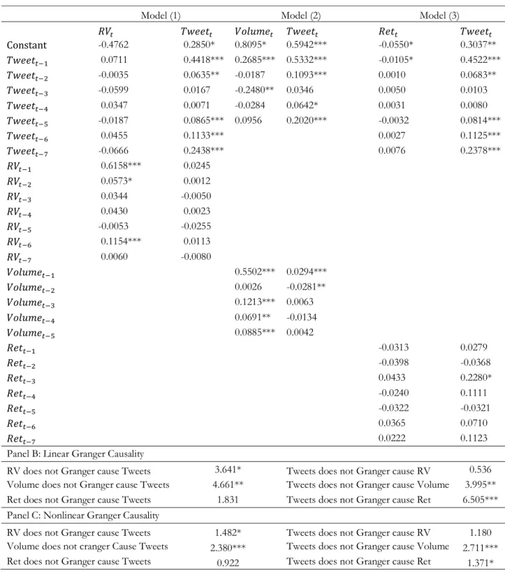
Panel B: Linear Granger Causality
RV does not Granger cause Tweets 3.641* Tweets does not Granger cause RV 0.536 Volume does not Granger cause Tweets 4.661** Tweets does not Granger cause Volume 3.995** Ret does not Granger cause Tweets 1.831 Tweets does not Granger cause Ret 6.505*** Panel C: Nonlinear Granger Causality
RV does not Granger cause Tweets 1.482* Tweets does not Granger cause RV 1.180 Volume does not cranger Cause Tweets 2.380*** Tweets does not Granger cause Volume 2.711*** Ret does not Granger cause Tweets 0.922 Tweets does not Granger cause Ret 1.371*
Table 3: This table reports the VAR estimation results for the first subsample period where each model examines the relationship between the number of tweet and RV, volume and returns respectively. The lag length is selected by the Schwarz Information Criterion. In Panels B and C, we report the linear Granger causality results, as well as the nonlinear Granger causality test of Diks and Panchenko (2006). ***, **, * indicate significance at the 1%, 5% and 10% levels respectively.
9
Table 4: This table reports the VAR estimation results for the second subsample period where each model examines the relationship between the number of tweet and RV, volume and returns respectively. The lag length is selected by the Schwarz Information Criterion. In Panels B and C, we report the linear Granger causality results, as well as the nonlinear Granger causality test of Diks and Panchenko (2006). ***, **, * indicate significance at the 1%, 5% and 10% levels respectively.
Model (1) Model (2) Model (3)
𝑅𝑉# 𝑇𝑤𝑒𝑒𝑡# 𝑉𝑜𝑙𝑢𝑚𝑒# 𝑇𝑤𝑒𝑒𝑡# 𝑅𝑒𝑡# 𝑇𝑤𝑒𝑒𝑡# Constant -4.4700*** -0.5331 -0.1641 0.1776 -0.0770 0.2738 𝑇𝑤𝑒𝑒𝑡#2- 0.5123*** 0.5278*** 0.8408*** 0.6449*** 0.0030 0.7092*** 𝑇𝑤𝑒𝑒𝑡#2* 0.0633 -0.0125 -0.3687 0.0556 -0.0200 0.0126 𝑇𝑤𝑒𝑒𝑡#2J -0.4877*** -0.0963 -0.4207* -0.0262 0.0528* -0.0634 𝑇𝑤𝑒𝑒𝑡#2K 0.1297 0.1565** 0.1757 0.1551** -0.0181 0.1138 𝑇𝑤𝑒𝑒𝑡#2L -0.0876 0.0063 0.3630* 0.2288*** -0.0105 0.2022*** 𝑇𝑤𝑒𝑒𝑡#2M 0.1200 0.1617** 𝑇𝑤𝑒𝑒𝑡#2N 0.0711 0.2930*** 𝑅𝑉#2- 0.3929*** 0.0444* 𝑅𝑉#2* 0.1370** -0.0268 𝑅𝑉#2J 0.1092* -0.0144 𝑅𝑉#2K 0.0911 0.0165 𝑅𝑉#2L 0.0147 -0.0428 𝑅𝑉#2M 0.0016 -0.0111 𝑅𝑉#2N -0.0515 -0.0048 𝑉𝑜𝑙𝑢𝑚𝑒#2- -0.5331 0.3327*** 0.0221 𝑉𝑜𝑙𝑢𝑚𝑒#2* 0.0162 -0.0420* 𝑉𝑜𝑙𝑢𝑚𝑒#2J 0.0518 -0.0151 𝑉𝑜𝑙𝑢𝑚𝑒#2K -0.0170 -0.0282 𝑉𝑜𝑙𝑢𝑚𝑒#2L -0.0618 -0.0253 𝑅𝑒𝑡#2- 0.0243 -0.1199 𝑅𝑒𝑡#2* 0.0256 0.0137 𝑅𝑒𝑡#2J 0.0157 -0.0526 𝑅𝑒𝑡#2K -0.0582 0.1464 𝑅𝑒𝑡#2L 0.0833 0.0936
Panel B: Linear Granger Causality
RV does not Granger cause Tweets 0.832 Tweets does not Granger cause RV 30.370*** Volume does not Granger cause Tweets 0.809 Tweets does not Granger cause Volume 24.650*** Ret does not Granger cause Tweets 1.883 Tweets does not Granger cause Ret 1.248 Panel C: Nonlinear Granger Causality
RV does not Granger cause Tweets 0.272 Tweets does not Granger cause RV 2.648*** Volume does not Granger cause Tweets -0.097 Tweets does not Granger cause Volume 2.678*** Ret does not Granger cause Tweets 0.317 Tweets does not Granger cause Ret 2.037**