Morphology is a Link to the Past: examining formative and secular galactic evolution through morphology

(1)

Morphology is a Link to the Past: examining formative

and secular galactic evolution through morphology

A THESIS

SUBMITTED TO THE FACULTY OF THE GRADUATE SCHOOL OF THE UNIVERSITY OF MINNESOTA

BY

Melanie A. Galloway

IN PARTIAL FULFILLMENT OF THE REQUIREMENTS FOR THE DEGREE OF

Doctor of Philosophy

Advisor: Lucy Fortson

(2)

(3)

Acknowledgements

Firstly, thank you to my advisor Lucy Fortson who supported and encouraged me throughout my graduate studies. Thank you also to my co-advisors Kyle Willett and Claudia Scarlata, who challenged me and pushed me to become a better scientist each day.

Thank you to everyone involved in the Zooniverse collaboration, especially everyone on the science team at Galaxy Zoo. Working with all of you has been a pleasure.

I am incredibly thankful for the support of my friends and family throughout this process. To Jill: thank you for the daily motivational thesis memes; they were great encouragement to keep writing! To White Tiger Martial Arts and all of the gumbros: thank you for providing me a place to relieve stress and feel connected to such a great community. To Nathan: thank you for editing my papers and reminding me that coffee stains make it look like you worked hard! To everyone who helped classify the FERENGI2 galaxies in Galaxy Zoo: thank you for saving my thesis! To the Sorin bums: thank you for putting up with me while I completed this. To Deadly Delights: thank you for giving me a reason to take a break from science for a whole week each year to spend with you wonderful people. To Zuko: thank you for being a nice cat.

Thank you to all of the graduate students who made graduate school fun, through the Dragon office, swords, board games, and good coffee.

Thank you to the Writing Center for hosting the 2017 Thesis Retreat. I learned so much about becoming a better writer and made significant progress on this thesis during the event.

None of the work in this thesis would be possible without the contributions of all of the Galaxy Zoo volunteers! Thank you for making science happen.

(4)

Galaxy morphology is one of the primary keys to understanding a galaxy’s evolu-tionary history. External mechanisms (environment/clustering, mergers) have a strong impact on the formative evolution of the major galactic components (disk, bulge, Hub-ble type), while internal instabilities created by bars, spiral arms, or other substructures drive secular evolution via the rearrangement of material within the disk. This thesis will explore several ways in which morphology impacts the dynamics and evolution of a galaxy using visual classifications from several Galaxy Zoo projects. The first half of this work will detail the motivations of using morphology to study galaxy evolution, and describe how morphology is measured, debiased, and interpreted using crowdsourced classification data via Galaxy Zoo. The second half will present scientific studies which make use of these classifications; first by focusing on the morphology of galaxies in the

local Universe (z <0.2) using data from Galaxy Zoo 2 and Galaxy Zoo UKIDSS. Last,

the high-redshift Universe will be explored by examining populations of morphologies

at various lookback times, fromz= 0 out toz= 1 using data from Galaxy Zoo Hubble.

The investigation of the physical implications of morphology in the local Universe will first be presented in Chapter 4, in a study of the impact of bars on the fueling of an

active galactic nucleus (AGN). Using a sample of 19,756 disk galaxies at 0.01< z <0.05

imaged by the Sloan Digital Sky Survey and morphologically classified by Galaxy Zoo 2 (GZ2), the difference in AGN fraction in barred and unbarred disks was measured. A weak, but statistically significant, effect was found in that the population of AGN hosts exhibited a 16.0% increase in bar fraction as compared to their unbarred counterparts at fixed mass and color. These results are consistent with a cosmological model in which bar-driven fueling contributes to the growth of black holes, but other dynamical mechanisms must also play a significant role.

Next, the morphological dependence on wavelength is studied in Chapter 5 by com-paring the optical morphological classifications from GZ2 to classifications done on infrared images in GZ:UKIDSS. Consistent morphologies were found in both sets and similar bar fractions, which confirms that for most galaxies, both old and young stellar populations follow similar spatial distributions.

(5)

of their age using classifications from Galaxy Zoo: Hubble (Chapter 6). The evolution

of the passive disc population from z= 1 to z= 0.3 was studied in a sample of 20,000

galaxies from the COSMOS field and morphologically classified by the Galaxy Zoo: Hubble project. It was found that the fraction of disc galaxies that are red, as well as the fraction of red sequence galaxies that are discs, decreases for the most massive galaxies

(log(M/M) > 11) but increases for lower masses. The observations are consistent

with a physical scenario in which more massive galaxies are more likely to enter a red disc phase, and more massive red discs are more likely to morphologically transform into ellipticals than their less massive counterparts. Additionally, the challenges of visual classification that are particular to galaxies at high redshift were investigated. To address these biases, a new correction technique is presented using simulated images of nearby SDSS galaxies which were artificially redshifted using the FERENGI code and classified in GZH.

(6)

List of Tables

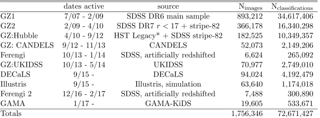
2.1 List of major completed Galaxy Zoo projects since 08/2017. All projects

have used optical images of galaxies, with the exception of UKIDSS

(in-frared, see Chapter 5). Nimages refers to the number of subjects classified

in the project, which may include duplicate unique galaxies (see data

release publications for details). Nclassifications refers to the sum of

clas-sifications received for each subject, not the number of clicks a subject

received (so a user answering 3 questions for a single galaxy would count as 1 classification, not 3). *Surveys included in HST Legacy are AEGIS,

COSMOS, GEMS, GOODS-N and GOODS-S single and 5-epoch. . . . 20

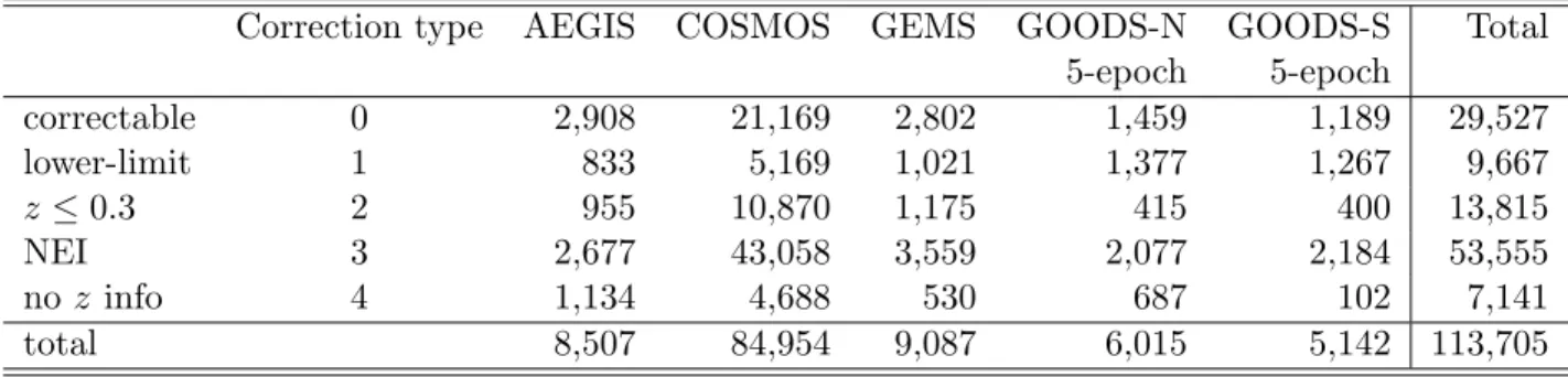
3.1 Number of correctable galaxies for the top-level task in GZH, split by

HST survey. . . 41

4.1 Summary of recent studies comparing the presence of galactic bars and

active galactic nuclei, including new results from this work. Martini et al. (2003) is the only study with neither uniform selection criteria for galax-ies nor a volume-limited sample. AGN classifications from optical line ratios and the BPT diagram are separated by the following demarca-tions: Ke01 = Kewley et al. (2001); Ka03 = Kauffmann et al. (2003c);

S07 = Schawinski et al. (2007). . . 58

4.2 Results of activity classification for our sample of 19,756 not edge-on disc

galaxies. ftotal is the percentage of the total sample represented by each

activity (number of galaxies of that type / total number of galaxies). fbar

is the percentage of each subsample that are barred (number of galaxies of that type that are barred / total number of galaxies in that type).

Errors are 95% Bayesian binomial confidence intervals (Cameron, 2013). 64

(11)

when splitting the sample in two by both mass and colour. fB>NB is

the fraction of bins that show an excess of barred AGN (compared to

unbarred), while dB−NB is the average value of the differences over all

bins. Since the number of bins in each subsample is only∼8−13 when

splitting by mass or colour, the uncertainty in fB>NB is correspondingly

large. . . 78

5.1 Comparison of depth and resolution of the UKDISS and GZ2 images.

The resolution between the two surveys is comparable, but the UKIDSS

images are an average of _∼1 magnitude shallower in all bands used to

create the color-composite images that where classified. . . 86

6.1 Net effects on the red disc fraction fR|D and red sequence disc fraction

f_D_|_R for limiting single-scenario cases of transformative pathways A, B,

C (Figure 6.12) and mass growth via star formation. ↑ represents an

increase in respective fractions with increasing cosmic time / decreasing redshift (right to left in Figure 6.11). This information can be used to find the dominant effects driving the trends in Figure 6.11. . . 141

6.2 Raw (unprimed) and corrected (primed) number counts of four

morphol-ogy/colour categories in four redshift bins for galaxies with stellar masses

within 10.1<log(M/M)<10.4. . . 149

within 10.4<log(M/M)<10.7. . . 149

within 10.7<log(M/M)<11.0. . . 150

within 11.0<log(M/M)<11.3. . . 150

(12)

List of Figures

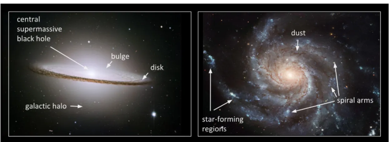
1.1 A side-on (left) and face-on (right) view of typical spiral galaxies. The

edge-on view gives a clear visual of the disk, bulge, and galactic halo com-ponents. The face-on view reveals the detailed spiral structure within the

disk. Left: Hubble image of Sombrero galaxy, M104. Credit: European

Space Agency. Right: Hubble image of Pinwheel galaxy, M101. Credit:

European Space Agency. . . 3

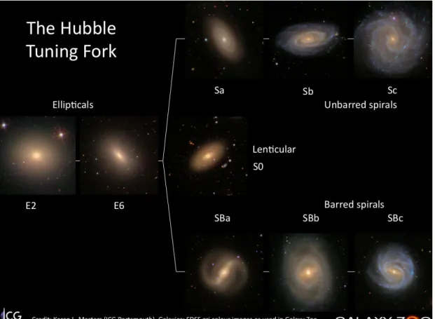
1.2 The Hubble Tuning fork with SDSS color-composite (gri) images as

exam-ples of the various types. Credit: Karen Masters and The Sloan Digital

Sky Survey (SDSS) Collaboration. . . 6

1.3 Color vs. Absolute Magnitude Diagram, illustrated using SDSS

galax-ies. In each color-magnitude bin, a random galaxy was selected meeting the criteria defined by that bin. The bottom-left and upper-right regions contain very few or zero galaxies, a consequence of typical galaxy evo-lution. As galaxies age and continue forming stars, they build up more stellar mass, increasing their total luminosity. Hence the most luminous galaxies tend to be older and more massive, and unlikely to be dominated by younger stellar populations. This results in a dearth of luminous blue

galaxies (bottom left) or faint red galaxies (upper right). . . 9

(13)

cal B-band (left), near-IR (middle), and mid-IR (right). Visible in the B-band image are patchy regions of star-formation and dust lanes, which become invisible in the near-IR, giving an overall smoother appearance. The mid-IR image shows regions where the dust re-radiates light absorbed from star-forming regions, giving a similar appearance to the optical

im-age. . . 10

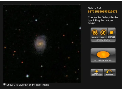
2.1 Example of the interface seen by users of Galaxy Zoo 1. On the left is an

image of a galaxy from the SDSS main sample. On the right are possible features the user may identify about the galaxy by clicking the relevant

option(s). Once complete, they are shown another galaxy. . . 16

2.2 Example of the interface seen by users of Galaxy Zoo 2. On the left is an

image of a galaxy, on the right are possible features the user may identify about the galaxy by clicking the relevant option. Unlike GZ1, subsequent questions appear about the same galaxy depending on their answers to the preceding questions, following a decision tree format (see Figure 2.3

for a visual of all possible pathways.) . . . 17

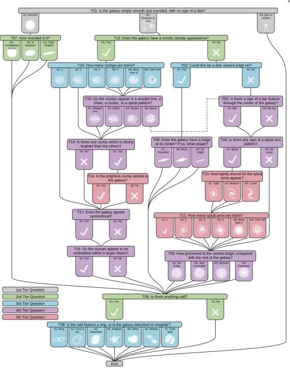
2.3 Decision tree used in the Galaxy Zoo:Hubble project. The colors indicate

the “Tier” level of the question. Gray represents 1st-Tier; these are asked of all users. Green are 2nd-Tier; these are only asked after responding to a 1st-Tier question, and so on. This tree is identical to GZ2 and UKIDSS,

except for the addition of the clumpy questions T12-T18. . . 18

2.4 Local ratios of morphologies for the first three tasks in the GZ2 decision

tree, used to derive debiased votes for the GZ2 sample. The full figure which includes baseline ratios for all tasks in the GZ2 decision tree is

shown in Willett et al. (2013), Figure 5. . . 23

(14)

of galaxies with vote fractions greater than 0.5 for each response to the first 3 tasks, where the solid lines are the raw vote fractions, dotted are the W13 debiased vote fractions, and dashed-dotted lines are debiased with the H16 method. As an example of the effect of the debiasing, see panel (a): without the debiasing, the number of galaxies with a “smooth”

majority vote fraction increases sharply fromz= 0.04 toz= 0.8, a range

assumed to be local enough such that no true morphological evolution should be observed. Both debiasing methods work to keep the fractions constant over this redshift range, although the H16 method is more

effec-tive at higher-tier questions. Bottom: Distributions of vote fractions for

the first answer to the first 3 tasks, for the low-redshift raw data (solid blue), higher redshift raw data (black solid line), W13 debiased (red thin-dashed line), and H16 debiased (red thick-thin-dashed line). Both methods are successful at shifting the high-redshift distributions to match the low-redshift distribution, with H16 being slightly more effective at matching

the shape of the distributions. . . 24

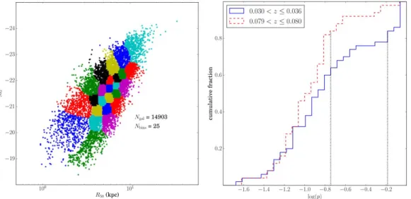
2.6 Credit: Hart et al. (2016), Figures 5 and 6. Left: Voronoi bin distribution

for the “> 4” answer to the spiral arm question in GZ2. Each bin is

further divided into Voronoi bins, such that each finalR50−Mr−z bin

contains at least 50 galaxies. Right: Cumulative distribution of vote

fractions (in log-space) of a single R50−Mr bin, split between a high

redshift bin (red dashed line) and a low redshift bin (blue solid line). The debiasing method adjusts the high-redshift vote fractions to match

the distribution of the low-redshift distribution. . . 27

3.1 Example of the redshift-induced bias in ffeatures. Five images of disc

galaxies from the GZH dataset are shown in order of increasing redshift,

from left to right. Above each galaxy is its redshift and below is itsffeatures

vote fraction. Although all galaxies appear to be discs with features, the vote fraction decreases steadily as redshift increases, as the details in each

image become more difficult to distinguish. . . 30

(15)

fer-engi code to produce simulated HST images. The measured value of

ffeatures from GZH for the images in each panel are (1) Top row: ffeatures

= (0.900, 0.625, 0.350, 0.350, 0.225) and (2) Bottom row: ffeatures =

(1.000, 0.875, 0.875, 0.625, 0.375). . . 35

3.3 Effects of redshift bias in 3,449 images in theferengisample. Each point

in a given redshift and surface brightness bin represents a unique galaxy.

On they-axis in each bin is theffeatures value of the image of that galaxy

redshifted to the value corresponding to that redshift bin. On thex-axis is

theffeatures value of the image of the same galaxy redshifted toz = 0.3.

The dashed black lines represent the best-fit polynomials to the data

in each square. The solid black line represents ffeatures,z=ffeatures,z=0.3.

Regions in which there is a single-valued relationship betweenffeatures at

high redshift and at z = 0.3 are white; those in which there is not are

blue, and those with not enough data (N <5) are grey. A larger version

of the bin outlined at z = 1.0 and 20.3 < µ < 21.0 (mag/arcsec2_{) is}

shown in Figure 3.4. . . 37

3.4 A larger version of the dark-outlined square in Figure 3.3, containing

ferengi galaxies that have been artificially redshifted to z = 1.0 and

have surface brightnesses between 20.3 < µ < 21.0 (mag/arcsec2_{). The}

orange bars represent the inner 68% (1σ) of the uncorrectable ffeatures

quantiles, which are used to compute the limits on the range of debiased

values. . . 38

3.5 Surface brightness as a function of redshift for 3,449ferengiimages and

the 102,548main galaxies with measured µand z values. The color

his-togram shows the number offerengiimages as a function ofµandzsim.

White contours show counts for the galaxies in the main sample, with

the outermost contour starting at N = 1500 and separated by intervals

of 1500. . . 40

(16)

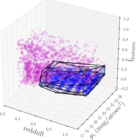
shift/surface brightness/ffeatures space. Pink points are all ferengi

galaxies in the unshaded regions of Figure 3.3. Blue points are all

ferengi galaxies in the blue shaded regions of Figure 3.3. The solid black line is the convex hull which encloses the uncorrectable points and

defines the region of the lower-limit sample. . . 42

3.7 Behavior of the normalised, weighted vote fractions of features visible

in a galaxy (ffeatures) as a function of redshift in the artificial ferengi

images. Galaxies in this plot were randomly selected from a distribution

with evolutionary correctione = 0 and at least three detectable images

in redshift bins ofz_≥0.3. The displayed bins are sorted byffeatures,z=0.3,

labeled above each plot. Measured vote fractions (blue solid line) are fit with an exponential function (red dashed line; Equation 3.4); the best-fit

parameter forζ is given above each plot. . . 44

3.8 All fits for the ferengi galaxies of the vote fraction dropoff parameter

ζ forffeatures as a function of surface brightness. This includes only the

simulated galaxies with a bounded range on the dropoff (−10< ζ <10)

and sufficient points to fit each function (28 original galaxies, each with varying images artificially redshifted in one to eight bins over a range

from 0.3.zsim.1.0). . . 45

3.9 Left: Debiased vs raw vote fractions for the GZH correctable sample.

The colorbar represents the number of galaxies in each bin. Right:

His-togram showing the fraction of galaxies that have a finite correction for

the debiased vote fractions ffeatures,debiased as a function of ffeatures and

redshift. The parameter space for corrections is limited to 0.3_≤z_≤1.0

due to the sampling of the parent SDSS galaxies and detectability in the ferengiimages. . . 46

(17)

the bulk r-band fits image for SDSS DR12 run 3903, camcol 6, and field 60. The boxed-in galaxy (SDSS DR12 objid 1237662239079268544) is too close to the edge of the image to create a cutout that encloses the entire

galaxy. The pink dashed box indicates a cutout size of 2*petroR90 r,

the blue solid line indicates a cutout size of 2.5*petroR90 r. . . 49

3.11 Examples of two galaxies whose minimum simulated redshifts inferengi

were larger than zsim = 0.3. These were detected via visual inspection

and removed from the finalferengi2 sample. . . 50

3.12 Examples of ferengi2 galaxies. The left is the original gri-composite

image of the source galaxy. Images on the right are simulated output

from the ferengi code. Only four of the eight simulated redshifts are

shown in the interest of space. . . 51

4.1 Examples of the SDSS images used in Galaxy Zoo 2, sorted by increasing

pbar(the weighted percentage of users that detected a bar in each image).

All galaxies are from our final analysis sample of “not edge-on” disc galaxies. The white lines in the upper left of each image represent a

physical scale of 5 kpc. We also give pbar and the SDSS objectIDs for

each galaxy. Top row: Galaxies with pbar< 0.3, which in this paper

are designated as unbarred. Middle and bottom rows: Galaxies with

pbar≥0.3, which we designate as reliably barred. . . 59

4.2 Left: Fraction of “not-edge-on” votes vs. inclination angle (i= cos−1[a/b])

for the disc galaxies in our GZ2 sample. An angle of 0◦means the galaxy

is completely face-on, while 90◦is completely edge-on. GZ2 users consider

a galaxy as “not edge-on” if the inclination angle is less than i _∼ 70◦.

Right: Fraction of barred galaxies vs. fraction of “not edge-on” galax-ies. The bar fraction is independent of the edge-on degree of the galaxies

(above pnotedgeon ∼0.3); the ability of users to detect bars does not

de-crease with inclination until pnotedgeon ∼ 0.3, or i ∼ 70◦. Error bars

are 95% Bayesian binomial confidence intervals (Cameron, 2013). This demonstrates that GZ2 data can reliably identify bars even in

moderately-inclined disc galaxies. . . 62

(18)

galaxy with S/N<3 for [Oiii], Hβ, [N ii], or Hα is unclassifiable using this method and labeled as “undetermined”. The 3,619 undetermined galaxies do not appear on the diagram above. The remaining 16,137 galaxies were categorized according to the above diagrams in the following order, based on the method of Schawinski et al. (2007). First, diagram (a) was used to identify star-forming and composite galaxies. Any galaxy below the Ka03 line was classified as star-forming, while those that fell between the Ka03 and Ke01 lines were classified as composite. Next, to distinguish AGN from LINERs, we use diagrams (b) and (c). If a galaxy had S/N > 3 for [O i], diagram (c) was used. If a galaxy did not have

S/N > 3 for [O i], but did for [S ii], diagram (b) was used. Last, if a

galaxy did not haveS/N >3 for [Oi] or [Sii], but did for [Nii], diagram

(a) was used. In each panel, only galaxies withS/N >3 for all four lines

required by that diagram are shown. Galaxies designated AGN by any of the three optical line diagnostics are plotted as blue points, while the

black shading represents the full sample of emission-line galaxies. . . 65

4.4 Mass and colour distributions for disc galaxies in the GZ2 sample,

sepa-rated by both activity type (either AGN or star-forming as in Table 4.2) and the presence of a galactic bar. AGN (green) are on average both significantly redder and more massive than star-forming galaxies (blue). When splitting the disc galaxies into barred (solid lines) and unbarred (dashed lines), however, there is no significant difference between the two populations. Counts are normalized so that the sum of bins is equal to 1

for each sample. . . 66

4.5 Optical colour vs. stellar mass for disc galaxies in GZ2. Black contours

represent all disc galaxies (top), all barred galaxies (middle), or all un-barred galaxies (bottom). All AGN (top), un-barred AGN (middle), and unbarred AGN (bottom) are plotted in the left panels as blue dots; the right panels show the AGN fraction in each colour/mass bin. Bins with

NAGN <10 are masked. . . 68

(19)

GZ2. Coloured bins show the difference between the AGN fractions for barred and unbarred galaxies. Blue bins have higher fractions of barred galaxies, red bins have more unbarred galaxies, and pale/white indicates no difference. The region on the colourbar enclosed by the dotted lines represents the mean of the data determined by the Anderson-Darling test. The colour gradient is on the same scale as Figure 4.5. Bins with

NAGN < 10 are masked. A colour version of this plot may be found in

the electronic edition of the journal. . . 69

4.7 Distributions of the difference in the fraction of bins with excesses of

barred AGN (fB>NB) and the average difference between barred and

un-barred AGN fractions (dB−NB). Both values are computed for 400

vari-ations in the mass and colour bin widths. Left: The average fraction

of bins with a higher barred AGN fraction is fB>NB = 0.705±0.073.

Right: The average difference in barred and unbarred AGN fractions

is dB−NB = 0.015±0.004. Dashed black lines indicate the values of

fB>NB and average dB−NB used in Figure 4.6 and subsequent analysis. . 70

4.8 Fits of the binned fraction of barred vs. unbarred AGN fractions to a

normal distribution. Left: value of the Anderson-Darling test (A2) as

a function of the standard deviation of the normal distribution being

fit (σd). The horizontal black line shows the critical value of A2

corre-sponding to 95%; a model must fall below this line to be considered an acceptable fit at this level of confidence. Two models are shown: the null hypothesis (blue diamonds) and the best fit to the data in Figure 4.6

(purple triangles). Right: Plot of the minimum A2 _{for the full range of}

means (dB−NB) tested for the data. This shows that acceptable fits can

be found for 0.005<dB−NB<0.019, but that the null hypothesis is ruled

out at 95% confidence. . . 71

(20)

unbarred (red) AGN in our sample. R is plotted as the mean of values

within five equal-width bins in the range 9.8<log(M/M)<11.3, which

includes 98% of the AGN sample. Points are drawn at the midpoint of

each bin. Right: Rvs colour for barred and unbarred AGN.Ris plotted

as the mean of values within five equal width bins in the colour range

1.6<(u−r) <3.0, which includes 96% of the AGN sample. Error bars

for each plot are 95% confidence intervals, calculated by bootstrapping with 1000 times resampling. There is no significant difference in accretion strengths for barred and unbarred AGN as a function of either mass or

colour. . . 75

5.1 Example of a galaxy whose morphological change between optical and

IR wavelengths was driven by a lack of light detectable in the IR relative to optical. This image was classified as featured and spiral in the optical using GZ2 vote factions (left), but smooth in the IR using UKIDSS vote

fractions (right) (dr7objid: 587726014553587781). . . 87

5.2 Example of ther₃J/r₂r_petrocalculation of one galaxy (dr7objid=587722981747392587).

Top Left: The sky-subtracted background of the J-band images are fit

to a Gaussian to derive the noiseN, which is given as the standard

de-viation of the fit. Top right: The signal to noise profiles of the J-band

images. The radius at which the signal-to-noise falls below three is

indi-cated by the green dashed line, and the thresholdS/N = 3 is indicated

by the horizontal black dashed line. The blue line shows twice the r-band

petrosian radius rr₂_petro for comparison. Bottom: Color-composite of

the optical gri image (left) and IR YJK image (right). The dashed circles

represent the radiusrr₂_petro (left) andrJ₃ (right), derived as shown in the

top row. The ratio of the two radii is given, showing that for this galaxy,

the light in the IR image extends to 62% of the optical image. . . 89

5.3 Example optical gri (left) and IR YJK (right) images of galaxies, sorted

by rJ

3/r2rpetro .The circle on the optical image (left) shows rr2petro, and

circle on the IR image (right) shows the J-band radius within which

(S/N)J >3, rJ3. . . 90

(21)

ues of rJ₃/r₂r_petro, where the light detectable in the J-band extends to a

significantly smaller area than the r-band images. Left: Distribution of

the change inffeatures from GZ2 to UKIDSS as a function ofrJ3/r2rpetro .

Right: The average change inffeaturesfrom GZ2 to UKIDSS as a function

ofrJ

3/rr2petro . The shaded region indicates the 1-σdispersion around the

mean. The dashed line atrJ₃/rr₂_petro = 0.75 indicates the threshold below

which galaxies are excluded from the comparison sample, due to the cov-erage of light in the J-band not reaching a significant area as represented

in the r-band. . . 91

5.5 IR images of galaxies tend to have a looser appearance of arms and more

prominent bulges than in optical images. Shown is the difference between

optical and IR ftight armsas a function of optical/GZ2 ftight arms(left), and

difference between optical and IR fobv+dom as a function of optical/GZ2

fobv+dom (right) for 502 galaxies which were classified as spiral in both

IR and optical images. The colors represent the fraction of galaxies that populate any given bin, and bins which could not represent a possible

difference in vote fraction (∆f > f or ∆f < f ₋1) are colored black.

The blue dotted line in both represents a difference in vote fraction of 0, such that galaxies below the line have larger IR vote fractions for the

feature represented in each plot, respectively. . . 93

5.6 Flow diagram showing the breakdown of morphologies in the UKIDSS

sample. Left: 6,484 galaxies in the volume-limited sample. Right: 279

SONIs: galaxies which were classified as spiral in the optical GZ2

classi-fications but do not follow the spiral path in the UKIDSS classiclassi-fications. 96

5.7 Example images of galaxies which were classified as spiral in optical GZ2

classifications but followed the “smooth” path in the UKIDSS

classifica-tions. . . 97

5.8 Example images of galaxies which were classified as spiral in optical GZ2

classifications but followed the “featured, not edge-on, no spiral” path in

the UKIDSS classifications. . . 97

(22)

classifications but followed the “featured, edge-on” path in the UKIDSS

classifications. . . 98

5.10 Example images of galaxies which were classified as spiral in optical GZ2 classifications but were classified as star/artifact in the UKIDSS

classifi-cations. . . 98

5.11 The middle bar displays the 421 galaxies which are classified as barred in both GZ2 and UKIDSS. To the left shows the number of galaxies

classified as barred in GZ2 butnot UKIDSS (blue). From left to right,

these are broken down by those that changed classifications because they followed the smooth path, featured, on path, and featured, not edge-on path (but with insufficient votes at the bar questiedge-on to allow a barred classification), respectively. To the right shows the number of galaxies

classified as barred in UKIDSS but not GZ2 (red). These are broken

down in the same way as described for the GZ2-classified bars. The total

number of bars detected combining both bands is 1,102. . . 99

5.12 Left: Flow diagram of UKIDSS-barred galaxies through the first three

GZ2 tasks. Right: Flow diagram of GZ2-barred galaxies through the

first three UKIDSS tasks. Most UKIDSS-barred galaxies are classified as featured, not edge-on galaxies in GZ2. Those which change classifica-tions to unbarred in the optical do so at the bar question; 22% of these

have vote fractions lower than the threshold fbar ≥ 0.3 required for bar

classification. Similar is true for GZ2-barred galaxies, although _∼ 20%

change classifications to unbarred in the IR because they initially follow the “smooth” path or “featured, edge-on”, without making it to the bar question in the first place. Of those which reach the bar question, 25% do

not achieve significant bar votes (fbar≥0.3) to allow a bar classification. 100

5.13 Galaxies classified as barred in UKIDSS (top row, IR images) and un-barred GZ2 (bottom row, optical images). The left column is an example of a galaxy which was not classified as barred in GZ2 because it followed the smooth GZ2 path, the middle followed the featured, edge-on path, and the right followed the featured, not edge-on path. . . 102

(23)

barred GZ2 (bottom row, optical images). The left column is an example of a galaxy which was not classified as barred in UKIDSS because it followed the smooth UKIDSS path, the middle followed the featured, edge-on path, and the right followed the featured, not edge-on path. . . 103 5.15 GZ2 vs UKIDSS bar strengths of 1,107 featured, not edge-on galaxies

measured by fbar. Galaxies shown must have 10 people answer the

bar question, ffeatures ≥ 0.35 and fnot edge−on ≥ 0.6 in both samples.

The dotted white lines indicate the threshold value for bar classification

fbar ≥0.3; the top-right region therefore displays the fraction of

galax-ies classified as barred in UKIDSS and GZ2, the bottom left are those classified as unbarred in both, the top-left are UKIDSS-barred and GZ2-unbarred, and the bottom-right are GZ2-barred and UKIDSS-unbarred. Most galaxies have consistent classifications (76% are either barred in both or barred in neither), 11% are barred in UKIDSS but not GZ2 (top

left) and 13% are barred in GZ2 but not UKIDSS (bottom right). . . . 104

5.16 u-r colors of 203 galaxies with bars detected in UKIDSS but not GZ2 (red) and 430 galaxies with bars detected in GZ2 but not UKIDSS (blue). The bars detected in the infrared but not optical images have redder colors than those detected in optical, suggesting dust obscuration may play a role in increasing the difficulty in visually identifying bars in optical

images. A two-sided KS test yielded a p-value p < 0.01 for the color

distributions of the two categories, rejecting the null hypothesis that the

samples were drawn from the same distribution. . . 107

(24)

defined as 0.2< z <1.1 and 10.1<log(M/M)<11.3. Blue cloud (left-panel) and red sequence (right-(left-panel) galaxies are plotted separately to illustrate the difference in limiting magnitudes for galaxies whose fluxes are dominated by I-band vs. V-band light respectively. The redshift cut was chosen to ensure morphological classifications are reliable, and the stellar mass cut was chosen to ensure a complete sample of both red

sequence and blue cloud galaxies out toz= 1. Left: Black contours show

counts for the blue cloud sample, with the outermost contour starting at

N=200 and separated by intervals of 200. Right: Black contours show

counts for the red sequence sample, with the outermost contour starting

at N=50 and separated by intervals of 50. . . 118

6.2 Evolution of colors using stellar population synthesis models. Galaxy was

assumed to have formed atz= 6 for plotting purposes. . . 119

6.3 The effect of reddening for highly inclined galaxies. On the left panel is

the distribution of fedge−on,no, which is the fraction of Galaxy Zoo users

who voted “no” in response to the question “Could this be a galaxy viewed edge-on?”. This vote correlates with inclination angle, such that low values represent highly inclined galaxies, and high values represent face-on galaxies. The bins are colored such that darker blue bins have a higher fraction of highly inclined galaxies, and white bins have high fractions of face-on galaxies. There is an obvious bias towards redder

colours for galaxies with high inclination angles (low votes for fedge−on,no).

We therefore implement a cut of fedge−on,no >0.3 to ensure that observed

red colours are an indicator of a lack of star formation, and not dust-reddening (right panel). . . 121

6.4 Separation of the passive population (red sequence) and active population

(blue cloud) of theferengi2 sample. The gray shaded region represents

the R-J limit of the sample. Combining the limit of r < 17 that was

adopted for the GZ2 dataset (of which theferengi2 galaxies are a

sub-set), with the 2MASS magnitude limit of J < 15.91, yields a limiting

colour for theferengi2 sample R−J <1.1. . . 124

(25)

ferengi code. The left image in each row is a real SDSS gri-composite image; the

four to the right are images generated by ferengi at varying redshifts,

processed to mimicHST /COSM OS imaging. Theffeatures vote fraction

for each simulated image is given; this value tends to decrease for each galaxy as it is processed to be viewed at higher redshifts. . . 125

6.6 Example calculation of completeness/contamination ξD/ξE at redshift

z= 0.7. Points represent GZ classifications of ferengi2 images. The

y-axis corresponds to the value offfeaturesmeasured at the galaxy redshifted

toz= 0.7, and the x-axis corresponds to the value offfeatures measured

at the galaxy redshifted to z = 0.3. On average, the ffeatures is lower at

the higher redshift, indicating classifiers on average have more difficulty identifying features in images modelling higher redshifts. The dotted

lines correspond to the threshold ffeatures=0.3, above which a galaxy is

considered to have a disc. Galaxies to the right of the vertical dashed line

were identified as discs at the lowest redshiftz= 0.3. The total number

of such galaxies is denoted Ndiscs true, and is defined to represent the true

number of disc-like galaxies. Galaxies above the horizontal dash line were

identified as discs at the higher redshiftz= 0.7, and their total number

is denoted Ndiscs detected. The ratio ξD = Ndiscs detected/Ndiscs true is the

completeness value; in this example, only 61% of discs were detected at

z= 0.7. Conversely, a contamination of 1.16% of ellipticals were detected.

Errors on the displayedξD andξE are 95% Bayesian binomial confidence

intervals (Cameron, 2013) . . . 127

(26)

RD BD RE BE

(bottom) as functions of redshift for red sequence and blue cloud

fer-engi2 galaxies separately. All show a clear dependence on ξ with

red-shift, but there is no strong difference in completeness for the red and

blue populations. Right: Completeness ξD (top) andξE (bottom) as a

function of redshift for all ferengi2 galaxies (red and blue combined).

The equation representing the linear fit for each is displayed. Shaded regions represent the 95% Bayesian binomial confidence intervals around

each point (Cameron, 2013). . . 128

6.8 No observed dependence on completeness ξ with surface brightness at

fixed redshift. Shown isξ vsµ in bins of redshift for blue cloud galaxies

(average values of ξ in each redshift bin are shown in Figure 6.9, right

panel). Linear fits were computed in each bin, shown as the dashed black

lines. Low overallR2 values and large p values, displayed in the legends

of each panel, suggest surface brightness does not have a strong effect on

completeness. The final calculation forξwas therefore only a function of

redshift. . . 129

6.9 Completeness ξ as a function of redshift and surface brightness for red

sequence (left) and blue cloud galaxies (right). In each redshift bin, galaxies were binned by surface brightness in varying widths such that Ndetected+ Ntrue ≥ 10 in each bin. The completeness ξ was computed

in each z, µ bin, represented by the colors. Darker colors represent a

completeness of 1, such that all disks were detected, while fainter colors represent a completeness near 0, representing a failure to detect disks.

ξ tends to decrease with redshift, but no correlation of ξ with surface

brightness is observed at fixed redshift. . . 130

(27)

open stars), red discs (red closed stars), blue ellipticals (blue open circles), and red ellipticals (red closed circles). Each point represents the fraction of the indicated type with respect to the total population, such that all points in a given redshift, mass bin sum to 1. Statistical errors were calculated as propagations of multinomial counting errors and the errors

associated with the functional fits to the correction terms ξD and ξE.

Systematic errors were calculated by bootstrapping the classifier votes for each galaxy and re-calculating the fractional contributions of each

type; errors were taken as the 1σ dispersion in the fractions. The total

error, represented by the shaded regions, is the statistical and systematic errors added in quadrature. . . 133 6.11 Left: Red disc fraction (f_R_|_D = N_RD0 /(N0_RD + N0_BD), equation 6.5) vs

redshift in four mass bins. Right: Red sequence disc fraction (fD|R =

N0_RD/(N0_RD+ N0_RE),equation 6.6) vs redshift in four mass bins.

Statisti-cal errors were Statisti-calculated as propagations of multinomial counting errors and the errors associated with the functional fits to the correction terms

ξD andξE. Systematic errors were calculated by bootstrapping the

clas-sifier votes for each galaxy and re-calculating the fractional contributions

of each type; errors were taken as the 1σ dispersion in the fractions.

The total error, represented by the shaded regions, is the statistical and systematic errors added in quadrature. . . 134 6.12 Cartoon representing three common evolutionary pathways of star-forming

disc galaxies. Path A represents an active star-forming galaxy which quenches without destroying the disc, becoming a red disc. Path B rep-resents a red disc morphologically transition to red elliptical. Path C represents a blue discs simultaneously quenching and morphologically transforming to become a red elliptical. . . 137

(28)

BD→RD BD→RE RD→RE

and κRE for four mass bins. The units for all rate parameters is Gyr−1.

25 equally-spaced values were tested between (0,1) for each parameter,

with the exception ofκRE which was tested for 25 values between (-1,1);

these are represented by the 25 bins on each axis. Each bin is weighted by

1/χ2_{, such that white regions correspond to parameters which produced}

the lowest χ2, and black representing the highest. There is a strong

re-sult in the dependence ofrBD→RD with mass, such that the fraction of

blue discs which transition to red discs (ie, quench without disrupting the disc), increases for more massive galaxies. The other parameters are less constrained by this model; therefore a more complex semi-analytic model will be necessary for obtaining the precise values of these rates, and is the subject of future work. . . 147

7.1 Resolution of the instrument has a strong impact on the physical

ap-pearance of a galaxy, and large differences could change a morphologi-cal classification drastimorphologi-cally, even for nearby galaxies. Shown is a spiral

galaxy at z = 0.1, imaged by SDSS at ∼.4”/pixel (left), and HST at

∼.04”/pixel (right) (HST Program ID 14606, PI: Simmons). The strong

bar and distinct spiral arms in the HST imaging are mostly lost in the

low-resolution ground-based image. . . 152

(29)

Chapter 1

Introduction

The clues to galaxy formation and evolution are hidden in the fine details of galaxy structure.

Peng et al., 2002

The processes which govern the formation, growth, and eventual death of galaxies are uniquely difficult to investigate. A galaxy cannot ever be directly observed from its birth to its death; the only data available is a single snapshot of the Universe as it exists at the moment of observing, in its current cosmological state. To begin to map out the complete evolutionary history of a galaxy, astronomers must instead use other clever, indirect methods.

One of the most powerful tools for revealing the physical processes that shape the evolution of galaxies is their morphology. Morphology refers to the visual appearance of a galaxy, which is set by the distributions of its stellar orbits. Particular features may include (but are not limited to) disks, rings, bars, clumps, or spiral arms. What determines which of these features develop in a given galaxy (or, what determines the particular stellar distribution of a galaxy,) is the galaxy’s dynamical history, which encompasses environmental interactions, star formation histories, and influences from dark matter and AGN. Specifically, details of a galaxy’s structure are known to be linked with its color (Tully, R.B., Mould, J.R., Aaronson, 1982; Strateva et al., 2001; Baldry et al., 2004), recent star-formation (Conselice, 2006; Martin et al., 2007a; Mignoli

(30)

et al., 2009), merger rate (Hammer et al., 2009; Oesch et al., 2010; Smethurst et al., 2017), and black hole activity (Athanassoula, 1992; Friedli & Benz, 1993; Schawinski et al., 2010), among others. There is no debate today that morphology is strongly linked to galactic evolution, but the extent to which these relationships hold is still difficult to quantify. Morphological classifications on scales large enough for results to claim statistical significance have been, in the past, unavailable. While expert visual classifications succeeded in accuracy, they lacked in numbers, and the opposite has been true for computational methods.

The research described in this thesis examines the link between morphology and evo-lution using data from the Galaxy Zoo project, which uses crowd-sourcing to provide a “best-of-both-worlds” approach to morphological classifications. To date, over one million volunteers have identified the structures of over one million galaxies, providing the benefits of both visual inspection and large numbers. With these data, the ways in which morphology drives (or is driven by) a galaxy’s evolution has been investigated on a scale previously unachievable. Three topics will be considered in detail: the influence of bars on AGN activity (Chapter 4), the dependence of observed wavelength on tracing different stellar populations (Chapter 5), and the interplay between quenching

mecha-nisms and morphological transformations of galaxies from redshift z _∼1 (Chapter 6).

This thesis also includes a detailed summary of the methodology used in collecting and reducing crowd-sourced data from Galaxy Zoo in the local Universe (Chapter 2) and introduces a new technique for debiasing high-redshift GZ classifications using data from simulated galaxies (Chapter 3). First, this Introduction will describe the typical components of a galaxy resulting from its formation, then give a brief summary of mor-phological types as have been defined historically, as well as the current evidence linking morphology to galaxies’ past histories.

1.1 Galaxy Formation

Galaxies are believed to have initially formed from primordial density fluctuations shortly after the Big Bang, as predicted by the ΛCDM model of Cosmology (Peebles et al., 1994; Ryden, 2006; Conselice, 2012; Silk et al., 2013). In this model, fluctuations

(31)

galactic halo disk bulge spiral arms dust star-forming regions central supermassive black hole

Figure 1.1 A side-on (left) and face-on (right) view of typical spiral galaxies. The edge-on view gives a clear visual of the disk, bulge, and galactic halo compedge-onents. The

face-on view reveals the detailed spiral structure within the disk. Left: Hubble image

of Sombrero galaxy, M104. Credit: European Space Agency. Right: Hubble image of

Pinwheel galaxy, M101. Credit: European Space Agency.

to the mean density of the Universe, ¯ρ: δ = ρ−_ρ_¯ρ¯. Gravitational instabilities will cause

even small perturbations (δ << 1) to grow exponentially with time; as δ _→ 1, the

region collapses and breaks off from the expanding universe, becoming a self-gravitating structure.

The collapse of these protogalactic regions of overdensity triggered the formation

of the first stars and galaxies around z ∼ 11, about 400 thousand years after the Big

Bang. At this time in the early Universe’s history, the only baryonic matter in existence

was Hydrogen and Helium, in a ratio of H : He _∼ 4 : 1. The very first stars to form

in the first proto-galaxies were thus comprised of only these two elements; for this reason they are classified as “extremely metal-poor stars” (EMPs), or Population III stars. Heavier elements formed later in the cores of EMPs, allowing for the formation of the metal-rich stars more commonly observed in galaxies today. As such, different populations of stars are often classified by their metallicity, measured by the amount of heavier elements they contain relative to Hydrogen [Z/H]. Population II stars have

metallicities of [Z/H] <0.1%; while they are still considered metal-poor, the presence

of any metal requires that they were formed from gas generated from the deaths of the earlier Population III stars. Population I stars are the youngest observed, with

(32)

metallicities [Z/H]_∼2₋3%.

The structure and components of a typical galaxy are shown in Figure 1.1. Most galaxies are believed to form with a disk component (Kormendy & Kennicutt, 2004), which is a product of the dynamics governing the initial galaxy formation. As large gas clouds cool and collapse, conservation of angular momentum causes the cloud to flatten and increase rotation speed, resulting in a disk shape. Young, Population I stars tend to form in the spiral arms of the disk, and particularly dense regions of star formation can give the arms a patchy appearance. Most galaxies are believed to contain a supermassive black hole in the center; while not observed directly, their influence on the galaxy in the form of feedback has been intensely studied (see Chapter 4 for details). Surrounding the black hole and often taking up a significant part of the galaxy is the central bulge, which tends to be comprised of older Population II stars. Both the disk and the central bulge can be destroyed as the galaxy evolves, transforming the galaxy’s morphology into a purely elliptical structure. It is believed that this morphological evolution is tied to the shutting-down, or quenching, of star-formation, due to ellipticals tending to host only older stellar populations (see Chapter 6). Permeating the galaxy is the largest observable component: the galactic halo, which contains gas which fuels ongoing star-formation, and stars which extend to the outer regions of the galaxy. Last, all of the luminous components are embedded in a dark matter halo, which cannot be observed directly, but interacts with the baryonic matter gravitationally.

While the preceding describes the elements of a typical galaxy, this does not begin to describe the wide range of morphological features that can be found. Disk galaxies for instance may have any number of spiral arms or no arms at all, or show evidence of rings or bars. Many galaxies do not even exhibit disk or elliptical structure at all but instead have irregular or clumpy appearances. This next section will describe in more detail the variances in the shapes of galaxies, and how the different structures are grouped into morphological classifications.

1.2 Morphological Categorization of Galaxies

The oldest and most well-known system which categorizes galaxies based on their struc-ture was developed by Edwin Hubble, commonly known as the “Hubble Tuning-Fork”

(33)

(Hubble, 1926). Using a small sample of images of nearby galaxies, Hubble identified two fundamental morphological classes: spirals, which exhibited well-defined disk struc-ture and clear spiral arms, and ellipticals, whose light distributions were smoothed over a roughly spherical shape. Only 3% of the sample had structures which deviated from these two categories, showing no evidence of rotational symmetry about a dominating nucleus; these were grouped together and labeled “Irregular”. Although Hubble’s sys-tem was originally based on a mere 400 galaxies, the classifications are still used for describing the morphologies of the millions of galaxies identifiable today (albeit with some modifications, e.g. DeVaucouleur’s revised system (de Vaucouleurs, 1963)).

An example of Hubble’s Tuning Fork is shown in Figure 1.2. The classifications defined on the Tuning Fork are as follows:

1.2.1 Ellipticals

The left side of the tuning fork contains elliptical galaxies, labeled “E”. These were orig-inally identified as circular through flattened ellipses whose luminosity faded smoothly from the center to “indefinite edges.” The only other structural feature evident to

sub-divide this class were their ellipticities, defined in the traditional way e= (a−b)/a. A

number is added to the label that represents the ellipticity, with the decimal omitted,

whereby E0 would represent a purely spherical elliptical (e= 0), and E7 being the most

elongated (e= 0.7). Hubble assumed that any galaxy with an ellipticity higher than 0.7

was no longer an elliptical, but more likely a highly-inclined spiral. It should be noted

that these labels only classify the projected appearance; since ellipticals are tri-axial

structures, this classification system is very dependent on the orientation angle of any ellipticals which are not perfectly spherical.

1.2.2 Spirals

The right side of the fork contains the various types of spiral galaxies. These all share the feature of having a flattened disk-shape, and often have a spherical bulge of stars in the center with spiral arms extending outward. Spirals whose arms originate from the central bulge follow the top of the fork, labeled “S”, while those whose arms originate at the ends of a central galactic bar follow the bottom, labeled “SB”. Both types are

(34)

Figure 1.2 The Hubble Tuning fork with SDSS color-composite (gri) images as examples of the various types. Credit: Karen Masters and The Sloan Digital Sky Survey (SDSS) Collaboration.

(35)

further classified based on the relative size of the central bulge and tightness of the arms. Those with large bulges and tighter arms are designated with an “a” attached to the spiral symbols, or “b”-“d” for decreasing bulge sizes and looser appearance of arms.

1.2.3 Lenticulars/S0s

Lenticular galaxies are placed at the center of the tuning fork, originally thought to be a transition stage to link the elliptical and spiral types. They exhibit the same overall disk-shape as the spirals, but have a smooth appearance rather than defined arms (which can make them difficult to distinguish from true ellipticals). They may or may not contain a galactic bar, giving them Hubble-type classifications of S0 (unbarred) or S0B (barred).

Hubble originally referred to the galaxies toward the left and right on the fork as “early” or “late”-type, respectively, simply for convenience in describing their relative positions on the sequence. While it is noted in his 1926 paper that any temporal connotation should be disregarded, the terms remain misleading in that it is now well-known that the early types tend to have older stellar populations, and late-types tend to be very young in their evolution. Nevertheless, “early-type” and “late-type” are still today used interchangeably when referring to ellipticals/S0s and disks.

1.3 Morphology as a tracer of galaxy evolution

The previous section describes the most common morphological types of galaxies ob-served in the Universe. At this point it may be relevant to question why are there different types at all? Do the different shapes exhibit different evolutionary pathways, or is the snapshot we see of the distributions simply showing different stages of a track that all galaxies eventually follow? The answers to these questions aren’t fully known; however, examining the relationships between the different morphological types and their dynamics can provide strong insights to the full picture. This section will pro-vide some examples of well-known links between morphology and galaxies’ evolutionary histories.

(36)

1.3.1 Color-Morphology Bimodality

The color of a galaxy is a strong indicator of its recent star formation history. In general, optically blue galaxies are in the process of forming new stars, emitting high energy blue light that is detected abundantly in short-wavelength filters. In contrast, galaxies which have ceased forming stars sometime in the past contribute most of their flux to long-wavelength filters, resulting in redder colors. Perhaps surprisingly, there is also a strong correlation between the color of a galaxy and its morphology. The majority of galaxies

(∼80%) have been shown out toz∼1 to follow this relationship: blue galaxies tend to

be late-type spirals, and red galaxies tend to be early-type/elliptical (Tully, R.B., Mould, J.R., Aaronson, 1982; Strateva et al., 2001; Baldry et al., 2004; Conselice, 2006; Martin et al., 2007a; Mignoli et al., 2009). An example is shown in Figure 1.3.1. The vertical

axis tracks the u₋r color, such that larger values are “redder” and smaller values are

“bluer”. The horizontal axis tracks the absolute magnitude: more luminous galaxies towards the left, and dimmer towards the right. Bluer galaxies tend to have more featured morphologies; spiral arms appear more flocculant and clumps of star formation are apparent, generating irregular shapes in the extreme cases. Redder galaxies begin to have a much more smoothed-out and symmetric appearance, encompassing both ellipticals and bulge-dominated lenticulars. Color has long been considered such a strong indicator of morphology that it has been often used as a proxy for morphology when large-scale visual inspection has not been practical (Cooray, 2005; Lee & Pen, 2007; Salimbeni et al., 2008; Simon et al., 2009). This link is strong evidence that the processes which drive both morphology and the cessation of star formation are related in some way (Masters et al., 2010; Buta, 2013). This topic is explored in greater detail in Chapter 6.

1.3.2 Morphology and Stellar populations

At the most basic level, morphology is simply a tracer of the observed distribution of light in the galaxy, which in turn traces the distribution of stars, gas, and dust. All light is not emitted equally, however: younger, Population I stars will emit more light in optical and UV wavelengths, while older Population II stars emit more strongly in the infrared. Since these populations may have very different spatial light distributions, there is inherently some dependence on morphology with the wavelengths within which

(37)

-24.0 0.8 -23.2 -22.3 -21.5 -20.7 -19.8 -19.0 -18.2 -17.3 -16.5 -15.7 -14.8 1.0 1.3 1.5 1.7 2.0 2.2 2.4 2.7 2.9 3.1 3.4

absolute magnitude M

z,petro

u

−

r

color

Figure 1.3 Color vs. Absolute Magnitude Diagram, illustrated using SDSS galaxies. In each color-magnitude bin, a random galaxy was selected meeting the criteria defined by that bin. The bottom-left and upper-right regions contain very few or zero galaxies, a consequence of typical galaxy evolution. As galaxies age and continue forming stars, they build up more stellar mass, increasing their total luminosity. Hence the most luminous galaxies tend to be older and more massive, and unlikely to be dominated by younger stellar populations. This results in a dearth of luminous blue galaxies (bottom left) or faint red galaxies (upper right).

(38)

Figure 1.4 Credit: Buta (2013), Figure 2.51. Spiral galaxy M51 observed in optical B-band (left), near-IR (middle), and mid-IR (right). Visible in the B-band image are patchy regions of star-formation and dust lanes, which become invisible in the near-IR, giving an overall smoother appearance. The mid-IR image shows regions where the dust re-radiates light absorbed from star-forming regions, giving a similar appearance to the optical image.

it is observed.

Morphologies observed in optical bands are sensitive to pockets of star-formation regions, but other features can be obscured due to dust extinction, particularly those comprised of older stellar populations (such as bars); this can give galaxies an overall “patchy” appearance. In contrast, they appear smoother in the near-IR, where the effects of dust extinction are reduced and the older stellar populations dominate. An interesting effect occurs as the observation wavelength moves into the mid-IR: here, dust tends to re-radiate the light absorbed from star-formation regions, re-creating the appearance of the optical-band morphology. There has been debate as to whether the optical and near-IR morphologies are de-coupled to the extent that two classification schemes, one for each wavelength range, is justified (e.g. Block & Puerari (1999)). Chapter 5 will examine the optical and near-IR morphologies measured by Galaxy Zoo to add to this debate, as well as investigate whether bars are in fact easier to identify in the near-IR.

(39)

1.3.3 Morphology and Environment

A galaxy’s environment can also be a predictor of its morphology. The morphology-density relationship, first quantified by Dressler (1980), observes an abundance of ellip-tical/ early-type morphologies in denser environments (de Souza et al., 1982; Postman, M. Geller, 1984). Since the merger rate correlates with environment density, it could be suggested that early-types are often the by-products of mergers, as opposed to a stage of isolated secular evolution.

There is also evidence of an environmental impact on morphology even in the absence of direct merging. For example, ram pressure (Gunn & Gott, 1972) exerted by the local intracluster medium can severly distort the gas distribution in a galaxy, resulting in asymmetries in the disk (ex. NGC 4402; see also Chapter 6).

1.3.4 Bars

Galactic bars are found in an estimated 30%-60% of spiral galaxies (Sellwood & Wilkin-son, 1993). They are elongated structures passing through the center of their host galaxies, and primarily dominated by older stellar populations (Eskridge et al., 2002) which often gives them a redder appearance with respect to the disk, which tends to be bluer from star-forming components in the spiral arms (see the “SB” types in the bottom row of the diagram in Figure 1.2 for example images of galaxies containing bars). Buta (2013) describes barred galaxies as “the ultimate in galaxy morphology.” His reasoning is simple: just by observing an image of a bar, it is easy to identify it as a major perturbation in an otherwise stable system. There is a great deal of truth in this; such a disruption will no doubt have significant effects on the fate of its host galaxy. In this way, bars are arguably one of the most important structural features that can shape a galaxy’s evolution.

A key feature of bars is their ability to drive gas from the outer regions of the galaxy to the center (Athanassoula, 1992; Friedli & Benz, 1993; Sellwood & Wilkinson, 1993; Shlosman et al., 1989; Ann & Thakur, 2005), which can affect the galaxy’s evolution in numerous ways. One such consequence is the formation of a pseudo-bulge (Kormendy & Kennicutt, 2004; Sheth et al., 2005). While this is seen in simulations, this theory is difficult to confirm observationally, as the bar may or may not be destroyed by this

(40)

process (Athanassoula et al., 2005), causing difficulty in identifying a correlation between populations of galaxies with both bars and bulges.

An increased inflow of gas to the center may also increase central star-formation. Several studies have reported an increase in star-formation rates in the central region of barred galaxies vs. their unbarred counterparts (Hawarden et al., 1986; Ho et al., 1997), although this may only be true for strong bars. Martinet & Friedli (1997) and Zhou et al. (2014) find low rates of star-formation in galaxies with weak bars, suggesting they are unable to trigger significant star formation. Galaxies with strong bars, however, show both the highest and lowest rates of star-formation. (Sheth et al., 2005) found a significant portion of barred galaxies with no molecular gas detected in the nuclear region, which may suggest that for these galaxies, the bar has already driven most of the gas to the nuclear region, where it was consumed by star-formation. Bars, then, seem to play two important roles in the star formation history of their host galaxies -both by increasing star formation, and subsequently driving the quenching process.

Bars also may be one of the mechanisms which enable the fueling of an active galactic nucleus (AGN), whose evolution is believed to be strongly linked to that of their host galaxies (Schawinski et al., 2007, 2010; Antonini et al., 2015; Yang et al., 2017; Zubovas & Bourne, 2017) (and Heckman & Best (2014) for a comprehensive review). The requirements for onset of accretion onto the central SMBH are still unclear, but Moles et al. (1995) argues that non-axisymmetric components of the gravitational potential may be a necessary condition; a requirement which bars easily satisfy. While simulations have shown bars to provide the necessary inflow to ultimately fuel an AGN (Athanassoula, 1992; Friedli & Benz, 1993), observations have shown mixed results. Many have found an excess of AGN in barred samples of galaxies (Knapen et al., 2000; Oh et al., 2012), while others find no difference (Ho et al., 1997; Mulchaey & Regan, 1997; Cheung et al., 2015). A discussion of the discrepencies between these results, along with my own investigation of this topic, is the subject of Chapter 4.

The examples listed are only a few of the well-known relationships between the evolu-tion of galaxies and their morphologies. There is little doubt amongst astronomers that morphology and galactic evolution are linked; however, as evident in these examples, some links are still inconclusive and the research of these relationships is still ongoing. Results are becoming more defined now, as methods to classify galaxies according to

(41)

their morphologies are constantly improving. Some of the results listed from previous decades suffered from low-sample statistics, where it was only feasible to visually classify handfuls of galaxies in a single study. Today, more robust methods are able to categorize galaxies morphologically in a fraction of the time once required. The next section will explore the evolution of classification methods used to obtain galaxy morphologies for such studies.

1.4 Methods for morphological classification

Historically, morphological classification has been done by visual inspection of small samples of images (e.g. Hubble (1926); Sandage (1961); de Vaucouleurs (1963); Block et al. (1994); Eskridge et al. (2002); Buta et al. (2010)), by either a single person or hand-ful of experts. This method is becoming obsolete as we enter a new era of large data, with surveys such as the Sloan Digital Sky Survey (SDSS) and HST-Legacy surveys, in addition to the upcoming James Webb Space Telescope, the Large Synoptic Sur-vey Telescope, and Euclid, producing high-quality images of hundreds of thousands of galaxies. To date, the largest morphological catalogs created by visual inspection from a small group of experts includes the Nair and Abraham catalog (Nair & Abraham, 2010)

with _∼ 14,000 galaxies, RC3 Catalog (de Vaucouleurs, 1991) with _∼ 23,000 galaxies,

and MOSES (Schawinski et al., 2007) with 50,000 galaxies. Even these catalogs, while successful, do not compare in size to the newly incoming data, and so more powerful and robust efforts are required to obtain morphological information on these scales.

An ideal method for handling the large amounts of data would be an automated classification scheme. Several such algorithms have been developed, with some success (Odewahn et al., 2002; Peng et al., 2002; Conselice, 2003; Scarlata et al., 2007) by using the stellar light distribution of the galaxy to assign it a morphological class. These approaches tend to be limited to identifying the global morphologies (ie, spiral or elliptical), and lack the precision to accurately identify finer, detailed features (such as bars or the number of spiral arms) (Beck et al., 2017). Further, they tend to incorporate proxies for morphology as their input, which are often not reliable (as detailed in the next paragraph). Much more promising techniques are currently being tested which incorporate the use of machine-learning algorithms and neural networks (Dieleman et al.